1. Model Development and Validations for Surface Water Chloride
Monitoring in Massachusetts
Dung T. N. Bui
Intern, Massachusetts Department of Environmental Protection, Division of Watershed Management, Watershed
Planning Program
Abstract:
Scientific evidencehas shown that the use of road salts can impact organisms and ecosystems. Widespread use of
road salts as a deicer has led to significantly high concentrations of chloride in many locations in Massachusetts
(Heath and Belaval, 2010), sometimes exceeding the U.S Environmental Protection Agency’s chronic chloride
criterion and acute chloride criterion. Previous studies have shown strong correlations between specific
conductance (SC) and chloride levels in water, but are not necessarily appropriate to be used in Massachusetts.
The main objective of this study was to document the development of a reusable data analysis tool using historic
chloride and SC data from Massachusetts Department of Environmental Protection (MassDEP) that would allow
the estimation of in-stream chloride levels using SC data.
Using data collected statewide from 1994 to 2012, two separate models were generated- one for freshwater
(𝑅2
=0.9445, P<0.001) and one for coastal waters (𝑅2
=0.9951, P<0.001). Both of them show a strong linear
relationship between SC and chlorideconcentration.Model validations were done using freshwater data collected
by USEPA and saltwater data collected by USGS, respectively. The slopes of the best fit linear model for freshwater
and saltwater are 0.9709 and 1.0608 (P<0.001), respectively and they are both close to the 1:1 line. The chloride
assessment tool developed by MassDEP is therefore believed to be accurate and robust enough to theoretically
predict and monitor statewide chloride concentrations using SC as a surrogate.
1. Introduction
Because slippery roads are problematic for drivers, road salt is used for snow and ice control to maintain safe
drivingconditions and to improve public safety in the winter. Sodium chloride, which is comprised of sodium ions
(𝑁𝑎+
) and chlorideions(𝐶𝑙−
),is the primary agent used, and its mechanismis well-understood (Sanzo and Hecnar,
2006).When applied on icy roads,saltcreates a solution that has a lower freezing point than water and thus melts
the ice. Eventually, the bond between ice and pavement is broken, turning a solid and slippery ice-covered road
into a drivable one with slush on the surface (Hochbrunn, 2010). The lowest pavement temperature on which
sodium chloride works is 10℉, and it plays a key role in preventing ice formation on asphalt (Shi et al., 2009). In
1938 New Hampshire was the first state to use road salt. Other states soon followed, and 5,000 tons of salt were
spread on the nation’s highways in the winter of 1941-42 (Kelly et al., 2010). Demand for road salt increased
parallel with the expansion of the highway system after World War II. The application of NaCl-based road salt has
risen dramatically with an annual average application of 9.6 million metric tons/year in the 1980s to 19.5 million
metric tons in 2011 in the United States (Corsi et al., 2014). As a part of the northern section of the country which
is heavily affected by snowfall,Massachusetts applies a largeamount of road salton state roads with an average of
20 metric tons/lanekm/year in recent years (Mattson and Godfrey, 1994),a much higher rate than average annual
loading of 1.7-10.9 metric tons/lane km in the Northeast and Mid-Atlantic (Morgan et al., 2012). Road salt

2. dissolves in water and releases sodium and chloride ions which then undergo ion-exchange reactions with soil.
Urbanization is a main factor in increasing chloride concentrations (Trowbridge et al., 2010). In the United States,
the urban land cover was 61,000 𝑘𝑚2
in 1945 and it reached 247,000 𝑘𝑚2
in 2007 (Corsi et al., 2014). With an
increasing rate of urbanization, the application of road salt as a deicer is likely to increase.
Road salt, in fact, is a water pollutant. A high percentage of this deicing agent is removed by infiltration into
ground water, runoff over impervious surfaces, and passage through pipes, finally makes its way to water
resources such as groundwater aquifers,nearby streams and lakes (Morgan et al,. 2012). Five gallons of water can
be permanently polluted by only 1 teaspoon of road salt,and only dilution duringrainfall and snowmeltcan reduce
the concentrations (Fortin and Dindorf, 2006).A high concentration of sodium chloride in water creates pockets of
high water density that settle at the bottom of the water body, causing chemical stratification which can prevent
dissolved oxygen from the upper water layer from reaching the benthic sediments (Novotny et al., 2008). Lack of
oxygen in the bottom layer eventually creates conditions unable to support aquatic life. Plants are highly
susceptible to salt toxicity and a loss in invertebrate numbers and diversity is found more in water bodies that
receive drainagefrom salted roads (Mattson and Godfrey, 1994).Road saltals o poses greatrisks to soil by altering
pH and the soil’s chemical composition;italso affects aquatic biota by altering patterns of succession (Trombulak
and Frissell, 2000). A desirable concentration of sodium in drinking water is 20 mg/L; 73 public water supplies in
Massachusetts exceeded this level in 1986 (Mattson and Godfrey, 1994).
In 1988 the U.S. Environmental Protection Agency (USEPA) published “Guidelines for Deriving Numerical National
Water Quality Criteria for the Protection of Aquatic Organisms and Their Uses.” The procedures described in those
guidelines indicated that freshwater organisms should not be affected badly if a 4 day average concentration of
dissolved chloride does not exceed 230 mg/L more than once every three years (chronic exposures), and if an one-
hour average concentration does not exceed 860 mg/L more than once every three years (acute exposures) (U.S.
Environmental Protection Agency, 1988).
Chloride concentrations and specific conductance (SC) have been shown to be directly correlated, and chloride
concentrations can be estimated from SC by empirical relationships (Trowbridge et al., 2010). Previous studies on
the relationships between chloride concentrations and conductance are summarized in Table 1. There are two
problems with these studies that have inhibited implementation of SC measurement as a proxy for chloride
concentrations in water.
The primary problem is that different research groups have used different equations to show relationships
between chloride concentrations and collected SC data (Table 1). Table 1 shows 24 equations that produce
different values for SC at 230 mg/L and 860 mg/L chloride levels. For instance, the equation for chloride
concentrations in Southern New Hampshire Watershed is Y = 0.307 * X - 22.00 which yields the SC of 820.85
𝜇𝑆/𝑐𝑚 (microsiemens per centimeter) for chloride concentration of 230 mg/L and 2,872.96 𝜇𝑆/𝑐𝑚 for chloride
concentration of 860 mg/L. The equation from Shingle Creek in Minnesota is Y = 0.3788 * X - 225.31 which yields
the SC of 1,201.98 𝜇𝑆/𝑐𝑚 for chloride concentration of 230 mg/L and 2,865.13 𝜇𝑆/𝑐𝑚 for chloride concentration
of 860 mg/L. Moreover, 17 out of 24 regression lines have 𝑅2
< 0.90. For the 7 regression lines with 𝑅2
> 0.90, the
SC range for 230 mg/L chloride level is from -392 to 1,202 𝜇𝑆/𝑐𝑚 and the corresponding range for 860 mg/L
chloride level is from 812 to 3,629 𝜇𝑆/𝑐𝑚.
The second problem is that these models have not been validated. A second dataset should be developed to
confirm the precision of the equations. The differences among SC values studied by different groups can be
explained by the geology of the area though which the water runs such as differences in bedrock, stream
discharge, and level of development (USEPA, 2012).

3. In spite of the increasing chloride levels, only a few Massachusetts water bodies have been reported as impaired
(Trowbridge et al. 2010). The state of Massachusetts has not been ready to use the results summarized in Table 1
as a reason to monitor water bodies for violations. Hence the Massachusetts Department of Environmental
Protection (MassDEP) sought to develop a model based on historical data, and to use data collected by USEPA and
USGS as a second datasetto validatethe reliability of MassDEP’s model. The primary objective of this study was to
document the development of a robust model demonstrating the link between chloride concentration and SC for
use by the MassDEP Division of Watershed Management -Watershed Planning Program (DWM-WPP)’s in surface
water quality assessments.
2. Materials and Methods
2.1. Study area
In Massachusetts, 3,570 chloride concentration data points were collected from 481 stations statewide from
summer 1994 to fall 2012 (Figure 1). Among these stations, coupled water samples (N= 2,442) were taken from
249 stations in the period of June 7, 1995 to November 14, 2012 for SC measurement by probe (in the lab or in-
situ). Water samples were collected by staff from DWM- WPP, and analyzed by MassDEP William, X. at Wall
Experiment Station (WES) in Lawrence, Massachusetts. For chloride analysis, the argentometric titration method
(Standard Methods 4500-𝐶𝑙−
, B) was used for water samples collected from 1994 to 2006 and the automated
ferricyanide method (Standard Methods 4500-𝐶𝑙−
, E) was used for samples collected from 2007 to 2012 (APHA
2005). Eighteen out of 481 stations were considered as coastal water stations because they were either directly
affected by coastal tidal water intrusion or indirectly affected by sea spray and precipitation due to their short
distance from the coast.
Figure 1. Chloride monitoring stations and distribution in Massachusetts (N= 481).

4. Table 1: Equations and multiple regression results
Regression Water Source
Maximum
Specfic
Conductivity
(uS/cm) Equation
# of
Samples R-Squared
SC level for
chloride at
230 mg/L
SC level for
chloride at
860 mg/L References
#1
Diluted OSIL
Atlantic Seawater 35,000 Y = 0.5381 * X - 133.96 66 0.9845 676.35 1,847.08
Windsor et
al. 2011
#2
Diluted OSIL
Atlantic Seawater 2,000 Y = 0.3946 * X - 7.065 30 0.9887 600.82 2,197.49
Windsor et
al. 2011
#3
Southern New
Hampshire
Watersheds Not available Y = 0.307 * X - 22.00 649 0.97 820.85 2,872.96
Trowbridge
et al. 2010
#4
Dark Brook and
Auburn Water
District Wells Not available Y = 0.2864 * X - 21.9 37 0.9936 879.54 3,079.26
Heath, D.
2014
#5
Browns Crossing
and Barrows
Wellfield 30,100 Y = 0.3688 * X - 109.28 68 0.9932 919.96 2,628.20
Heath, D
and Morse,
D. 2013
#6
Diluted OSIL
Atlantic Seawater Not available
Y = 0.5231 * X +
435.077 30 0.9661 -392.005 812.24
Windsor, C
and
Mooney, R.
2008
#7 Bassett Creek 1,788 Y = 0.2412 * X - 74.372 31 0.4111 1,261.91 3,873.85
Bischoff et
al. 2009
#8 Bevens Creek 1,041 Y = 0.0566 * X - 7.8388 87 0.1867 4,202.10 15,332.84
Bischoff et
al. 2009
#9 Browns Creek 414 Y = 0.0013 * X + 19.533 9 0.0004 161,897.69 646,513.08
Bischoff et
al. 2009
#10 Carver Creek 1,035 Y = 0.0011 * X + 38.862 70 0.0002 173,761.82 746,489.09
Bischoff et
al. 2009
#11 Coon Creek 645 Y = 0.069 * X + 18.086 6 0.1087 3,071.22 12,201.65
Bischoff et
al. 2009
#12 Elm Creek 844 Y = 0.0192 * X + 38.068 55 0.0085 9,996.46 42,808.96
Bischoff et
al. 2009
#13
Lower Minnesota
River 1,823 Y = 0.1587 * X - 46.293 186 0.5483 1,740.98 5,710.73
Bischoff et
al. 2009
#14 Lower Rum River 523 Y = 0.1422 * X - 27.754 22 0.4044 1,812.62 6,243.00
Bischoff et
al. 2009
#15 Minnehaha Creek 7,890 Y = 0.0637 * X + 66.216 287 0.1389 2,571.18 12,461.29
Bischoff et
al. 2009
#16 Nine Mile Creek 2,726 Y = 0.2092 * X - 49.743 72 0.7849 1,337.20 4,348.68
Bischoff et
al. 2009
#17
Riley/Purgatory/Bl
-uff Creek 1,256 Y = 0.0317 * X + 27.713 28 0.0527 6,381.29 26,255.11
Bischoff et
al. 2009
#18 Sand Creek 1,633 Y = 0.1597 * X - 55.696 86 0.826 1,788.95 5,733.85
Bischoff et
al. 2009
#19 Shingle Creek 96,435 Y = 0.3788 * X - 225.31 138 0.9867 1,201.98 2,865.13
Bischoff et
al. 2009
#20
Six-Cities
Watershed 950 Y = 0.4543 * X - 205.32 3 0.8871 958.22 2,344.97
Bischoff et
al. 2009
#21 Sunrise River 278 Y = 0.0209 * X + 4.2037 7 0.4498 10,803.65 40,947.19
Bischoff et
al. 2009
#22 Upper Rum River 419 Y = 0.0767 * X - 7.4655 11 0.7542 3,096.03 11,309.85
Bischoff et
al. 2009
#23 Valley Branch 582 Y = 0.0097 * X + 14.118 51 0.0776 22,255.88 87,204.33
Bischoff et
al. 2009
#24 Vermillion River 1,514 Y = 0.1465 * X - 34.99 194 0.6045 1,808.81 6,109.15
Bischoff et
al. 2009

5. 2.2. Water sample collection and analysis
2.2.1. Water sample collection (chloride)
Samples were collected by trained DWM water quality personnel.Container labels provided information about the
identification,analysis and assessmentof specific samplinglocationsand were placed on the dry containers before
entering the field. When combined in the same bottle with other analysts (e.g. nutrients), chloride samples were
preserved with 1:1𝐻2 𝑆𝑂4. Wade-in manual grab samples were generally taken, but when wade-in sample
collection was notpossible,an extension sampler pole was used to avoid shore effects and ensure sampler safety.
The sample bottles were typically rinsed two to three times in ambient water before grabbing samples. The multi-
probes were deployed in the water first; samples were taken side-by-side, downstream of the multi-probe units.
The sampling containers were facing upstream and plunged into the water to about 6 inches below water surface
to avoid collecting surface scum. All samples were stored in insulated coolers packed with ice to achieve the
temperature of approximately 4℃ and transported to the WES laboratory. Non-Hg thermometer vials were used
to ensure that the temperature was maintained during the trip. The use of non-routine sampling techniques,
current climate, current site conditions, and observations were also noted on DWM fi eld sheets to help the
assessmentgroup and other analysismakedecisions aboutthe data collected. Water samplecollection was guided
by the MassDEP Standard Operating Procedure CN1.21 (Chase 2009) or previous versions.
2.2.2. Field Use of Hydrolab in collecting SC data
Multiprobe instruments were used to collect most of the SC measurements according to WES or DWM-WPP
standard operating procedures (SOPs). For the stations that were not wadeable, river and stream monitoring from
bridges was employed using an anchored guidelineassembly hungover the bridge wall or railing and releasing the
line slowly to the riverbed. The position of the anchor would remain unchanged and any plume of resuspended
sediments was sure to be carried downstream prior to collecting readings. Readings were recorded every 30
seconds for five minutes, after all enabled variables were stable. During colder months, recordings required
additional recording time due to certain multiprobe variables’ ability to reach equilibrium at cooler temperatures
(5-10℃). The last stable set of readings after 5 minutes were used as the grab data. All SC data were collected
under guidance of MassDEP SOP #4.24 (Chase et al. 2010) or previous versions.
2.2.3. Data quality assurance and quality control
In general, all field samples were collected under Quality Assurance Project Plans. Typically, the DWM-WPP
collected two types of samples for field quality control (QC): ambient field blanks and duplicate samples at a
minimum of 10% (for each type) of samples taken. Laboratory accuracy and precision were determined by the
policy and procedures in the WES Laboratory’s Quality Assurance Plan and Analysis Procedures. Laboratory
accuracy employed matrix spikes and performance evaluation samples, while laboratory precision involved
analysis of same-sample lab duplicates and matrix spike duplicates. The duplicate readings from Hydrolab
multiprobe (i.e., every 30 seconds for 5 minutes) provided information on overall precision or repeatability of the
in-situ measurements.
In order to transfer sample custody for all samples from DWM to WES laboratory, a standard chain-of-custody
(COC) form was used. DWM-WPP data were validated either by PrincipleInvestigators(1994-2000) or by WPP’s QA
Officer (2000-2012). Data were either accepted, qualified or censored based on the review. Only accepted and
qualified data were used in the development of the model.

6. 2.3. Model development and Statistical analysis
A Kolmogorov-Smirnov test was used to examine whether or not statewide SC data were normally distributed
(Daniel and Cross, 2012). Linear regression was used to develop the relationship between chloride concentrations
and SC in both freshwater and coastal waters. Analysis of covariance (ANCOVA) was utilized to analyze the
distinction between freshwater and coastal water models. The freshwater model includes the data with SC less
than 10,000 𝜇𝑆/𝑐𝑚. The coastal water model includes data with SC higher than 10,000 𝜇𝑆/𝑐𝑚, plus data from
stations alongthe coast. In Massachusetts,there is no inland freshwater station with SC values higher than 10,000
𝜇𝑆/𝑐𝑚 (Health and Morse, 2013;Health, 2014). Eighteen coastal stations were identified, but one of these was not
used in the model development because it could not meet QA/QC standard.
The freshwater model was validated using the USEPA Auburn field observation during winter 2013-2014 (Health,
2014). For the Auburn study, 37 freshwater samples were collected by the USEPA and analyzed for chloride
concentrations. The freshwater model developed by MassDEP was used to calculate predicted concentrations of
chloride. The predicted numbers generated by the MassDEP model were put on a best fit line with real data
collected from the USEPA study. The coastal water model was validated by comparing the USGS marine field
observations with the MassDEP coastal water model predicted values. Ten coastal samples collected by USGS in
Massachusetts from 2007 to 2012 were taken from the USEPA’s STORET Data Warehouse (USEPA 2014). A similar
validation procedure to the freshwater model was used to validate the coastal water model. All the statistics and
model estimation were performed using SAS® (Version 9.4, SAS Institute Inc. Cary, NC)
3. Results
3.1. Chloride Distribution in Massachusetts
There appears to be a strong correspondence between chloride concentrations and urbanized land in
Massachusetts in 2000 (Figure 1). In eastern and parts of Central Massachusetts, a high urban land cover is
associated with higher chloride concentrations of 100-859 mg/L. On the other hand, western and midwestern
Massachusetts,where the urban land cover is low, have lower chloride concentrations (mostly less than 99 mg/L).
This is likely due to increased road salt use in areas with urban land cover. Table 2 below provides more specific
information about chloride distribution from 26 watersheds in Massachusetts.
Table 2: MassDEP chloride monitoring (N= 481)
3.2. Model Development for Freshwater and Coastal Areas
All samples were used for a statewide linear model (N= 2,442). Although chloride and SC fit the model well
(𝑅2
=0.995), it is not adopted because the SC data are not normally distributed (Kolmogorov-Smirnov test, D=0.44,
P<0.01). There are only 15 points that are above 30,000 𝜇𝑆/𝑐𝑚, only 1 point between 10,000 and 30,000𝜇𝑆/𝑐𝑚,

7. and the rest 2,426 data points are below 10,000 𝜇𝑆/𝑐𝑚. The higher SC points are stations near coastal areas
(Figure 1), which might be directly or indirectly influenced by the sea. Analysis of covariance revealed that the
difference between the freshwater and coastal water models is significant (F= 216,094, P<0.001).
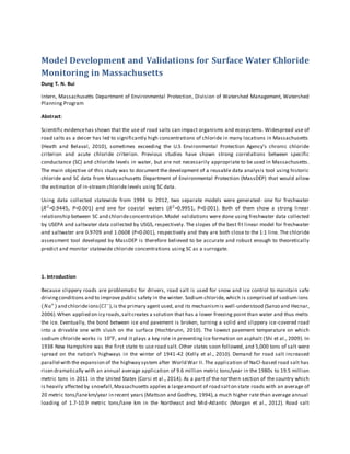
Samples collected from freshwater stations statewidegenerated a freshwater regression model as shown in Figure
2. Chloride concentrations [Cl] and SC show a strong linear relationship with an equation:
Y= 0.2753X – 18.987 with 𝑅2
=0.9445, P<0.001, N = 2,426 (Y=Chloride concentration [Cl], X=SC)
The lowest chloride concentration is 1.0 mg/L and the highest is 2,400 mg/L. Observed average chloride
concentration is 64.08 mg/L, 99th percentile is 250 mg/L, and 99.85% of the concentration values fall under 860
mg/L. SC values that are associated with the chronic and acute exposures of dissolved chloride are calculated by
plugging in Y=230 mg/L (chronic level) and Y=860 mg/L (acute level) into the equation, resulting in X = 904 𝜇𝑆/𝑐𝑚
and X = 3,193 𝜇𝑆/𝑐𝑚, respectively.
A strong linear relationship between chloride concentrations and SC in coastal water is also found (Figure 3):
Y= 0.3647X - 101.59 with 𝑅2
=0.9951, P<0.001, N= 63 (Y=[Cl], X=SC).
The lowest chloride concentration is 5.5 mg/L and the highest concentration is 18,000 mg/L. Observed average
chloride concentration is 4,124 mg/L and 75th percentile is 5,800 mg/L. According to the coastal water regression
model, a water body that exceeds a SC of 909 𝜇𝑠/𝑐𝑚 or 2,637 𝜇𝑠/𝑐𝑚 would be considered chronic exceedance
([Cl]=230 mg/L) or acute exceedance ([Cl]=860 mg/L), respectively. It is not surprising that the coastal region has
higher chlorideconcentrations becauseof sea spray,and seawater intrusion.In addition,the coastal area is highly
urbanized with heavy application of road salt in the winter which also leads to high chloride concentrations.
Figure 2. Relationship between chloride and SC for
Massachusetts’ freshwater samples.
Figure 3. Relationship between chloride and SC for
Massachusetts’ coastal water samples.
0
500
1000
1500
2000
2500
0 5000 10000
ChlorideConcentration(mg/L)
Specific Conductance (uS/cm)
0
4000
8000
12000
16000
20000
0 20000 40000 60000
ChlorideConcentration(mg/L)
Specific Conductance (uS/cm)

8. 3.3. Validation of Freshwater Model and Coastal Water Model
The freshwater model was validated by using the USEPA Auburn study data conducted during the winter 2013-
2014. The best fit line between MassDEP freshwater model predicted values and the observed USEPA chloride
concentrations (R2=0.9908, P<0.001) demonstrates that the model is accurate because 99.08% of the variation is
explained (P<0.001) and the regression line is close to the 1:1 Line with a slope of 0.9709 (Figure 4).
Similar resultswere obtained for validatingthecoastal water model. The MassDEP model predicted chloridevalues
strongly correlated with USGS measured chloride concentrations because 99.65% of the variations are explained
(P<0.001) and the regression line is also close to the 1:1 line with a slope of 1.0609 (Figure 5).
Figure 4. Validation on Freshwater Model using
USEPA Data.
Figure 5. Validation on Coastal Water Model using
USGS Data.
4. Discussion
4.1. Models developed by MassDEP
As mentioned in the introduction,other studies have developed models that show a relationship between chloride
concentration and SC. Nevertheless, none of them is considered appropriate for use in the state of Massachusetts.
After analyzing the factors that may cause variation among models, MassDEP developed its own freshwater and
coastal water models from historical data collected statewide. In order to prove that the models are highly
reliable, datasets from the USEPA Auburn study for freshwater and the USGS study for seawater were used to
validate the MassDEP models. The chloride concentrations predicted by our models are pretty close to the
observed concentrations, with the slope of 0.9709 for freshwater model comparison and 1.0608 for coastal water
model comparison (best fit line). We are confident that the models that we developed and validated are very
robust and ready to be used.
4.2. Implementation
The U.S. National Climate Assessment summarized the observed changes in the amount of precipitation falling in
very heavy events in the period of 1958-2012.The Northeast region shows a clear trend beyond natural variations

9. with a 71% increase in the amount of heavy precipitation (Melillo et al., 2014). As this trend continues, more road
salt is expected to be applied on impermeable surface out of concern for winter safety. As a consequence, the
concentrations of chloride will continue increasing especially during low flow seasons, and the impacts on
ecosystem will be amplified.
In 2014, the Massachusetts Department of Transportation (MassDOT) issued a Reduced Salt Policy to minimize
sodium and chloride effects on water resources (MassDOT, 2014). MassDEP is charge with ensuring clean water
includingcontrollinglevels of pollutants such as chloride, but the agency did not have a tool for managing chloride
in water bodies. With the development of two accurate models, chloride concentrations can be easily predicted
using its linear relationship with SC. According to the MassDEP models, a baseline for SC that meets chronic
exposure (230 mg/L of chloride concentration) and acute exposure (860 mg/L) levels is set for both fresh and
coastal water.
The two models developed are very important to the state of Massachusetts since they will assist in identifying
impaired waters. Furthermore, every state is different in terms of climate and geology, the MassDEP model can
serve as a prototype for other states to follow, or they may wish to develop their own model.
5. Conclusion
Our results show that 98.5% of the freshwater stations in Massachusetts possess chloride concentrations under
230 mg/L. According to Figure 3, stations with high chloride concentrations are all in urbanized regions with high
population densities. Collection of more data may identify additional impacted areas. Our data also indicate that
most chloride in the water comes from discharged road salt. The finding is not surprising as urban areas have
larger impervious surface area, but it confirms the results of earlier studies on the relationship between
urbanization and road salts.
For future work, MassDEP has been examining SC and chloride concentrations in River Meadow Brook and the
Concord River. Six HOBO U24 Conductivity Loggers have been deployed at six stations and data are uploaded once
a month. The conductivity readings arerawconductivity at ambient water. Samples for chloride are grabbed using
wade-in technique every time the field trip is made; they are preserved and transported to the USEPA New
England Regional Laboratory in Chelmsford, MA. Hydrolab multiprobes are used for QC purposes at a rate of once
a month atall six stationsto collect SC, temperatures, and TDS (Total Dissolved Solids) data. Conductivity data are
transformed to SC data for comparison purposes. The new project data will be available in 2016 and will provide
an extended data set based on continuous data from Fall through Spring. This new set of data will be used to
support the models that MassDEP developed from historical data.
The chlorideassessmenttool promises to be an effective tool for the state of Massachusetts to usein monitoring
and assessing chlorideconcentrations.
Acknowledgements
Support for this study was provided by the Massachusetts Department of Environmental Protection. I greatly thank
David Wong and Richard Chase who provided help with specific recommendations, comments, and
encouragement. I would like to thank all of our colleagues for collecting chloride data and providing technical
assistance,as well as GIS support. I also really appreciate data provided by USEPA and USGS for model validation.
Copyright of this document belongs to MassDEP.

10. References
Benoit, D. A., Stephan, C. E. (1988) Ambient Water Quality Criteria for Chloride. USEPA, Report EPA 440/5-88-001,
Office of Water, Regulations and Standards Criteria and Standards Division, Washington, D.C.
Bischoff, J., Spector, D., Brasch, R., Schultz, J., Schuck, J., Strom, J. (2009) Phase 1 Chloride Feasibility Study for the
Twin Cities Metropolitan Area. Minnesota Pollution Control Agency. Wenck Associates, Inc. Wenck File #0147 -200.
ChaseR (2009) Sample Collection Techniques for Surface Water Quality Monitoring. Massachusetts Department of
Environmental Protection Division of Watershed Management. Standard Operating Procedure # CN 1.21. 46 pages.
Chase R, Smith J, Chan L, Haynes B (2010) Water quality multi -probes. Massachusetts Department of
Environmental Protection Division of Watershed Management. Standard Operating Procedure # CN 4.24. 49 pages.
Corsi, S. R., De Cicco, L. A., Lutz, M. A., Hirsch, R. M. (2014) River Chloride Trends in Snow-affected Urban
Watersheds: Increasing Concentrations Outpace Urban Growth Rate and are Common among All Seasons. Science
of the Total Environment 508:488-497.
Daniel, W. W., Cross, C. L. (2012) Biostatistics: A Foundation for Analysis in the Health Sciences (10th Edition).
Wiley. 777 pages.
Fortin, C., Dindorf, C. (2006) Road Salt Education and Training for Those Maintaining Parking Lots and Sidewalks.
Pollution Prevention Grant. Final Report CFMS#A72150.
Heath, D., Belaval, M. (2010) Baseline Assessment of Stream Water Quality in the I-93 Tritown project Area from
December 1, 2009 to April 7, 2010. USEPA Region I New England, Preliminary Data Report, Boston, MA.
Health, D., Morse, D. (2013) Road salt transport at Two Municipal Wellfields in Wilmington, Massachusetts. New
England Water Works Association CXXVII: 1-23.
Health, D. (2014) Data Report Acute Road Salt Contamination of Dark Brook and the Auburn Water District’s
Church Street Wellfield in Auburn, Massachusetts. Office of Ecosystem Protection, USEPA New England Region 1,
Boston, Massachusetts 02109. 14 Pages.
Hochbrunn, S. (2010) Special Report: Clear Roads, Clear Issues - Journey into World of Winter Road Maintenance
Reveals Concerns, Conflicts, progress – and a Long-Simmering Dispute in one Massachusetts Town. The New
England Interstate Water Pollution Control Commission Interstate Water Report 7(1):1,4-17.
Kelly, V. R., Findlay, S. E. G., Schlesinger, W. H., Menking, K., Chatrchyan, A. M. (2010) Road Salt: Moving Toward
the Solution. The Cary Institute of Ecosystem Studies, Special Report, Millbrook, NY.
MassDEP 2010 Quality Assurance Program Plan Surface Water Monitoring & Assessment. Massachusetts
Department of Environmental Protection Division of Watershed Management 2010-2014. Control Number 365.0,
rev. 1. MS-QAPP-27. 183 pages.
Massachusetts Department of Transportation (2014) Reduced Salt Policy. MassDOT, S.O.P NO. HMD-01-01-1-000,
Massachusetts.
Mattson, M. D., Godfrey, P. J (1994) Identification of Road Salt Contamination Using Multiple Regression and GIS.
Environmental Management 18(5):767-773.

11. Melillo, Jerry M., Terese (T.C.) Richmond, and Gary W. Yohe, Eds. (2014) Climate Change Impacts in the United
States: The Third National Climate Assessment. U.S. Global Change Research Program, 841 pp.
doi:10.7930/J0Z31WJ2.
Morgan II, R. P., Kline, K. M., Kline, M. J., Cushman, S. F., Sell, M. T., Weitzell Jr., R. E., and Churchill, J. B. (2012)
Stream Conductivity: Relationship to Land use, Chloride, and Fishes in Maryland Streams. North American Journal
of Fisheries Management 32:941-952.
Novotny, E. V., Murphy, D., Stefan, H. G. (2008) Increase of Urban Lake Salinity by Road Deicing Salt. Science of The
Total Environment 406(1-2):131-144
Sanzo, D., Hecnar, S. J. (2006) Effects of road de-icing salt (NaCl) on larval wood frogs (Rana sylvatica).
Environmental Pollution 140(2):247-256.
Shi, X., Fay, L., Gallaway, C., Volkening, K., Peterson, M. M., Pan, T., Creighton, A., Lawlor, C., Mumma, S., Liu, Y.,
Nguyen, T. A. (2009) Evaluation of Alternative Anti-icing and Deicing Compounds Using Sodium Chloride and
Magnesium Chlorideas Baseline Deicers – Phase I. Colorado Department of Transportation. DTD Applied Research
and Innovation Branch. Report No. CDOT-2009-1. 270 pages.
Trombulak, S. C., Frissell, C. A. (2000) Review of Ecological Effects of Roads on Terrestrial and Aquatic
Communities. Conservation Biology 14(1):18-30.
Trowbridge, P. R., Sassan, D. A., Kahl, J. S., Heath, D., and Walsh, E. M. (2010) Relating Road Salt to Exceedances of
the Water Quality Standard for Chloride in New Hampshire Streams. Environmental Science & Technology
44(13):4903-4909.
USEPA (U.S. Environmental Protection Agency) (2012) Conductivity. USEPA, Washington, D.C. Available from:
http://water.epa.gov/type/rsl/monitoring/vms59.cfm (Accessed October, 2015)
Windsor, C., Mooney, R. (2008) Verifying the Use of SC as a Surrogate for Chloride in Seawater Matrices. 20 th Salt
Water Intrusion Meeting 155-158.
Windsor, C., Steinbach, A., Lockwood, A. E., Mooney, R. (2011) Verifying the Use of SC as a Surrogate for Chloride
in Seawater Matrices, Rev. 01 1-7.