The Impact of RBA Monetary Surprises -Chapman (2014)

The Impact of RBA Monetary Surprises
Blair Chapman∗
June 30, 2014
Abstract
Central banks used to be secretive organisations but over the last few decades they have
begun to release more information on their monetary policy decisions. For example, the Reserve
Bank of Australia (RBA) made changes to its communication policies in 2007, releasing minutes
from Board meetings and publishing media releases on the afternoon of interest rate decisions
for all meetings. My research measures how these announcements impact interest rate futures,
bond markets, equity markets, and currencies, using intradaily data. Gürkaynak, Sack and
Swanson (2005) use a high-frequency event study analysis to estimate the effects of two factors
on asset prices in the US; these two factors can be interpreted as news about the current policy
rate and news about the future path of policy in a central bank announcement. Following a
similar methodology I identify these factors in RBA announcements and estimate the impact of
the factors on financial markets.
Keywords: Monetary policy, Reserve Bank of Australia
JEL Classification: E52, E58, E43, G14
∗
Department of Economics, Johns Hopkins University, 440 Mergenthaler Hall, 3400 N. Charles St., Baltimore,
MD 21218; bchapma5@jhu.edu. I thank Jonathan Wright for his helpful advice, comments and suggestions. I also
thank the Reserve Bank of Australia for financial support and assistance with data. The views expressed are those of
the author and do not necessarily reflect those of the Reserve Bank of Australia. Responsibility for any errors rests
solely with the author.
1

1 Introduction
Central banks used to be secretive organisations but over the last few decades they have begun
to release more information on their monetary policy decisions. The Reserve Bank of Australia
(RBA) was no exception. For example in 1993, the then Governor of the RBA, Bernie Fraser said
releasing minutes of the Reserve Bank Board (RBB) meetings “would run a real risk of impairing
the Banks decision making”(Fraser, 1993 p.6). Fourteen years later the RBA began releasing min-
utes of the RBB meetings, albeit with a two week delay and less detail than Fraser had envisioned.
In this paper I examine the impact of RBA announcements on asset prices and whether changes in
communication policy have changed the impact that announcements have.
This paper contributes to the literature by being the first to measure the surprise in monetary pol-
icy for the RBA using futures. Other studies on Australian monetary surprises have used changes
in yields on 30-day Bank Bills or 90-day Bank Bills as the measure of surprise. This paper also
measures the surprise at tighter windows, using 30 minute, 1 hour, and daily windows around
announcements, rather than just daily windows.
In general, the findings are in line with economic intuition. I find that, on average, in the 30 minutes
around a surprise 25 basis point (bp) increase in the cash rate: the Australian dollar appreciates by
0.9 percent, equity indices fall 0.4 percent, and short-term government bond yields increase around
14 basis points (bps). I also find that monetary policy surprises around the Statement on Monetary
Policy (SMP) and minutes are related to larger market movements than the equivalent surprise
from a cash rate announcement.
In addition to using a single monetary policy factor, the possibility of multiple monetary policy
factors is investigated using the methodology of Gürkaynak, Sack and Swanson (GSS) (2005a).
While rank tests are unable to reject the hypothesis that a single factor is sufficient to explain the
response of asset prices to monetary policy announcements in the tighter windows, there is some
support for an additional factor at the daily window. The second factor appears to be tied to
expectations of the future path of policy.
2

The remainder of this section discusses the types of communications that could move Australian
financial markets and Section 2 discusses the related literature. Section 3 describes the data and
estimates the impact of a monetary policy surprises. Section 4 looks at the possibility that the
change in communication policy changed the impact of monetary policy surprises on financial
markets. Section 5 considers the level and timing components of a monetary surprise, while Section
6 explores the possibility that monetary policy announcements contain more than just one type of
surprise. Section 7 concludes.
1.1 RBB communications
It has now become typical for central banks to announce any changes in monetary policy. Between
1990 and July 1997 only 8 out of 22 changes in the cash rate came the day after the RBB meeting
(RBA, 1997). Between 1997 and 2007, the RBA announced changes in the cash rate the day after
the RBB meeting where the decision was made.1 This consistent announcement regime meant that
market participants could gauge a non-announcement to mean that the cash rate was going to
remain unchanged.
On 5 December 2007, the RBB announced that it would be changing its communication policy
(RBA, 2007). Beginning with the December 2007 meeting, the RBA began issuing press releases
after every board meeting. Before December 2007, press releases were only issued after a deci-
sion was made to change the cash rate target. Also in the 5 December 2007 press release, it was
announced that beginning with the February 2008 meeting, that the decision of the RBB would
be released at 2:30 pm the afternoon of the meeting, rather than 9:30 am the following morning.
Thirdly, the 5 December 2007 press release announced that minutes from RBB monetary policy
meetings would be released two weeks after the meeting. The first set of minutes released were on
5 December 2007 for the meeting held on 6 November 2007.
In addition to press releases, the RBA also issues a SMP four times a year, in February, May,
August, and November (RBA, 2000). The statements discuss the economic climate including
1
The content of each press release for this period is available on the RBA website.
3

possible inflation and growth with much more detail than the press releases.2 The SMP are released
at 11:30 am. Since February 2009 the SMP has been released on a Friday. Prior to February 2009,
the SMP was released on either on a Monday or a Friday. Table 23 contains a full list of SMP
release dates between 2001 and 2014.
1.2 Other macroeconomic announcements
The primary source for economic data in Australia is the Australian Bureau of Statistics (ABS).
The ABS produces the Australian national accounts, labour market data, sales data, construction
data, trade data as well as some select financial data. The ABS releases all data at 11:30 am the
day of the release. Due to the large volume of data produced by the ABS, it is common for the
ABS to release data on the same day as the RBA makes their monetary policy announcement.3
Between February 2001 and December 2013, the ABS released 421 publications on RBB cash rate
announcement days, 106 publications on SMP days, and 190 publications on Minutes days.4 Not all
of these publications are likely to lead to changes in financial markets. However, a not insignificant
proportion of the publications will influence the markets. Publications such as Australian National
Accounts and Government Finance Statistics are examples of two of the same day releases that
have the potential to influence financial markets. Measuring the monetary surprises and asset price
changes in a window that excludes the ABS releases should allow for better identification of the
surprise attributable to RBA announcements and the related movements in asset markets. Unfor-
tunately, a smaller window does not help in the case of SMP’s or Minutes as they are released at
the exact same time as ABS data.
Another source of information about the Australian economy is its Department of Treasury. It
releases various reports on regulations governing companies, government budgets and analysis of
the economy. It regularly releases an Economic Roundup which contains articles on the future path
of government policy on taxes and economic regulation, and other items pertinent to the Australian
economy. The Australian Department of Treasury does not release their Economic Roundup on a
2
Typically, SMPs are at least 17,000 words across more than 70 pages.
3
Between January 2001 and December 2013, there were only 7 monetary policy announcement days where the
ABS did not release any data.
4
A complete list of these publications is available from the author upon request.
4

Tuesday or Wednesday very often. They have only done it eight times since the beginning of 2000,
with two released on the Tuesday coinciding with RBA meetings. However, at that time the RBA
were releasing their monetary policy decision on the Wednesday. Since the beginning of 2000 the
Department of Treasury has released 9 reports, listed in table 1, which came out on the same day
as the RBA released their monetary policy decision.
In addition to being influenced by Australian data and policy the Australian markets are also
influenced by decisions and data from overseas. Craine and Martin (2008) found that Australian
markets are affected by decisions made by the US Federal Reserve (Fed) and other data coming
out of the US. US data typically comes out overnight in Australia. Australia’s other trade partners
and its close neighbours could also affect the domestic markets. However, as table 2 shows, most,
if not all, economic data related to Australia’s trade partners is released outside of the tight 30
minute window being examined here.
2 Related literature
The literature measuring surprises in data releases and announcements and their impact on various
markets is quite vast.5 A subset of this literature focuses exclusively on the impact of monetary
surprises; a large proportion of the studies focus on the Fed and its impact.
A strand of the literature focuses on measuring the size of movements in interest rates and asset
prices caused by changes in monetary policy. Early papers in this part of literature, such as Cook
and Hahn (1989), used changes in the target rate as the indicator of monetary policy. The liter-
ature has since moved to looking at the surprises contained in monetary policy announcements,
since the efficient market hypothesis suggests that markets should only react to the unanticipated
part of any announcement. Using deviations of the announced number from the median market
forecast as the measure of surprise was typical in the early literature on measuring surprises. Kut-
tner (2001) was one of the first to use Fed funds futures to measure policy expectations. He used
this surprise measure to estimate the impact of anticipated and unanticipated target rate changes
5
Faust et al (2007) contains a list of a number of these papers and summarises their findings for the US.
5

across the yield curve. He shows that the response to unanticipated changes is large and significant.
Bernanke and Kuttner (2005), using daily changes in Fed funds futures to measure surprises, exam-
ine the impact that changes in monetary policy by the Federal Open Market Committee (FOMC)
have on equity returns in the US. Using both the S&P500 and Center for Research in Security
Prices (CRSP) value-weighted returns they find that a surprise 100 bp cut in the Fed funds rate
leads to a 4.68 percent decrease in the one day return. Also using surprises measured with Fed
funds futures; GSS (2005) examine the impact of the Fed’s actions and announcements on the
S&P500 stock market indices and bond yields. In addition, using a group of futures they use factor
analysis to break the response of monetary policy into a current target factor and a future path
factor.
A second strand of the literature investigates the impact of surprises on exchange rates using an
event study approach. Zettelmeyer (2004) examines the impact of monetary policy surprises on the
exchange rate in Australia, Canada, and New Zealand and finds that a surprise 100 bp contraction
results in a 2 to 3 percent appreciation of the exchange rate. He uses daily changes in three month
Treasury bill rate to measure the surprise. Karagedikli and Siklos (2008) investigate the change
in the NZ$/A$ and NZ$/US$ caused by surprises in various releases by the Reserve Bank of New
Zealand and other macroeconomic data. They also decompose monetary policy surprises into what
they call a permanent and transitory component.
Faust et al (2007) examine the response of bond yields and exchange rates to 10 different macroe-
conomic announcements. They follow Kuttner (2001) and use changes in the Fed funds futures to
measure Fed surprises. They find that responses to positive surprises about US activity lead to
short-run appreciation of the US dollar.
Anderson et al (2003) look at the reaction of US, German and British stock, bond and foreign ex-
change markets to US macroeconomic news. Their study is broad and encompasses 25 US macroe-
conomic news announcements across 9 different markets and incorporates international spillover
effects. They measure surprises in news using deviations in median survey expectations from the
6

released number. They find that US announcement surprises have an impact both in the US and
abroad.
This paper like Anderson et al (2003) and Faust et al (2007) looks at more than one asset market
but restricts itself to a single country, Australia, and a single type of news, monetary policy. There
are a number of studies that have analysed the impact of monetary policy news in Australia on
a single dimension; most commonly the exchange rate. Kearns and Manners (2006) examine the
impact of monetary policy shocks on exchange rates for Australia, Canada, New Zealand and the
UK. They measure monetary policy shocks using the daily change in bank bill interest rates; they
use 30-day and 90-day rates.
Coleman and Karagedikli (2010), as part of a study examining spillovers from Australian economic
announcements to the New Zealand dollar, examine the reaction of the A$/US$ exchange rate
and the A$/NZ$ exchange responses to surprises in Australian monetary policy. They measure
monetary policy surprises using daily changes in the 30-day bank bill yield. They find that a 100
bp surprise in monetary policy leads to a 2.3 percent appreciation of the A$/US$ exchange rate
and a 0.75 percent appreciation of the A$/NZ$ exchange rate.
An early study looking at bond yields in Australia is Campbell and Lewis (1998). They looked at
the effects of a broad range of news events, including US news, to determine what moved Australian
bond yields from January 1994 to January 1997. Using pooled regressions with dummy variables
for announcement days, they examine whether the announcements lead to increased volatility in
yields. Campbell and Lewis also look at surprises using the deviation in the news release from
the median market forecast. They use changes in futures contracts on the 90-day bank bills and
10-year bonds to measure changes in interest rates. So the dependent variable in their work is the
explanatory variable used in this study. The period they examine also saw monetary policy an-
nouncements frequently occur off schedule, which means assuming that a non-announcement after
a meeting meant no change in the cash rate was a less valid assumption.
Clifton and Plumb (2008), following a similar methodology to Campbell and Lewis (1998), find that
7

volatility in the A$/US$ exchange rate jumps around times of monetary policy announcements in
a broader study on the volatility of the exchange rate around economic releases.
Craine and Martin (2008), using a linear simultaneous equations model and a factor model with
monetary and non-monetary factors, examine spillover effects between the US and Australia. They
examine all days from January 3, 1994 to December 31, 2003 using daily data. They use the 30-day
eurodollar rate as their shortest yield so they can have securities and with identical features across
the two countries. They find that the RBA affects the domestic market but not the US. They
also test the bias present in an event study specification and find it to be small but significant for
responses by the 30-day US eurodollar rate and exchange rate to their money surprises.
3 The effects of changes in the cash rate on asset prices
3.1 Data
To measure the surprise in RBA announcements, I use ASX 30-Day Interbank Cash Rate Futures
(cash rate futures).6 Similar to federal funds futures in the US, cash rate futures are contracts with
pay outs at maturity based on monthly average rates. The pay out on the cash rate futures are
based on the average Interbank Overnight Cash Rate published by the RBA. For weekends and
public holidays the overnight cash rate for the previous business day is used (ASX Limited 2014).
As is the convention for interest rate futures, the prices are quoted as 100 less the yield, where
the yield is percent per annum. The minimum price movement is half a bp or 0.005 percent (ASX
Limited 2014). The cash rate futures are available 18 months in advance with most of the trading
taking place closer to the expiry date. My data on cash rate futures runs from September 2003
to August 2013. The data is missing observations for a couple of contracts, leaving me with 108
observations of the surprise on RBB decision announcement days.
The markets I look at are Australian government bond markets, Australian equities and exchange
rates. I use daily and intraday bond yields to quantify the impact of RBA surprises on bond yields.7
6
5 min interval data was obtained from CQG Data for the cash rate futures.
7
Daily bond yields for the on-the-run Australian Treasury bond yields are available from Bloomberg L.P. 10
minute bond yields were obtained from the RBA’s Financial Markets Group, Domestic Market Department, Market
8

I use daily and intraday exchange rates to evaluate the impact of surprises on exchange rates.8 To
assess the impact of monetary surprises on equity markets I use daily data on the ASX and All
Ordinaries indices, and ASX sector indices.9
Another security that may be interesting in this analysis is the 90-day bank accepted bill futures
contract (90-day future). The 90-day future is available for March, June, September and December
each year, up to ﬁve years out (ASX Limited 2014). Other commonly traded futures are the 3-
and 10-year Treasury bond futures. Similar to the 90-day future the 3- and 10-year future are only
available for March, June September and December.10
If possible, three windows are created: 30 minute, 1 hour and daily. As discussed above, there are
a number of other non-RBA announcements that could possibly lead to market movements on any
day. The 30 minute window around cash rate decisions is a window that is free from almost all
other announcements. This allows me to identify the market movements that are a response to the
RBA and not some other source. The 30 minute window is measured from 10 minutes before an
announcement to 20 minutes after the announcement. For example, for an RBB cash rate decision
at 2:30 pm the 30 minute window begins at 2:20 pm and ends at 2:50 pm. 1 hour windows are taken
from 10 minutes before an announcement to 50 minutes after the announcement. Daily windows
are measured from the end of the announcement day to the end of the previous day.11
3.1.1 Does window size matter for measuring movements?
In the past, a number of authors have looked at the impact of monetary policy surprises at the daily
and longer windows for various countries. However, the use of daily data increases the possibility
of measurement error, since there are numerous other macroeconomic news announcements across
the period of analysis that could also lead to changes in asset prices. The use of intraday data
Operations team.
8
Daily data for exchange rates is available from a number of sources. 10 minute changes in exchange rates were
obtained from the RBA’s Financial Markets Group, International Department.
9
Daily data for the ASX and All Ordinaries indices is available from a number of sources. Daily data on the ASX
sub-indices were obtained from Thomson Reuters Eikon.
10
Tick by tick data was obtained for the 90-day, 3-year and 10-year futures from Tickdata.com.
11
The daily currency window is measured from the open of the Sydney trading day to the open of the following
Sydney trading day.
9

is going to give more precise estimates if there are large differences between movements measured
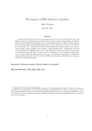
using a daily window and movements measured using smaller windows. As shown in figure 1, for
the monetary surprises calculated using the cash rate future there is little difference between the
30 minute and 1 hour windows. From figures 2 and 3 we can see that there are larger differences
between the short windows and the daily window. As table 3 shows, on cash rate decision days the
average absolute value of monetary surprises at the 30 minute window is 4.2 bps, the 1 hour window
average is 4.4 bps and the daily average is 4.6 bps. The average difference across days, between the
surprise at the daily window and the 30 minute window is 0.9 bps. The small difference between
the daily and tighter windows suggests that there is not a large amount of additional measurement
error if monetary policy surprises are measured at the daily window.
However, the measurement window appears to matter for the financial market variables. For the
1-year government bonds being analysed, changes in the 30 minute window and daily windows
are 3.8 bps different on average. The difference in the changes between windows is apparent in
figure 4. Other government bonds exhibit similar differences between windows but the change in
the 30 minute windows decline as the bond tenor increases. All of the exchange rates also exhibit
differences between changes measured at the daily window and changes measured at the 30 minute
window. The difference between the two windows for the US$/A$ exchange rate can be seen in
figure 5. This preliminary analysis indicates that there is a lot more noise in the changes measured
at the daily frequency than changes measured at the tighter windows. This noise leads to larger
measurement error in the daily window than the tighter windows.
The presence of the additional measurement error can be seen in the regression results in with
larger standard errors associated with the estimated coefficients using the daily window than the
30 minute window. While the tighter windows reduce measurement error, they may also fail to
capture the market’s reaction if an announcement takes time to interpret. This may be especially
true for the SMP and minutes due to the length of the documents market participants need to
analyse.
10

3.1.2 Example days
To see the impact an RBA cash rate decision can have on the markets it is useful to look at some
examples. To also illustrate the fact that sometimes not changing the cash rate can have an impact,
I will look at the contrasting examples of 2 February 2010 and 1 June 2010. On 2 February 2010
the RBB’s actions surprised the market and on 1 June 2010 they did not.
On 2 February 2010, the RBB decided to leave the cash rate unchanged after they had raised the
cash rate by 25 bps at each of its previous three meetings; from 3.00 to 3.75 percent. The majority
of market was obviously expecting another 25 bps increase at the February meeting with cash rate
futures at 96.08, or 3.92 percent. As figure 6 shows, immediately after the RBB announcement at
2:30 pm, the cash rate future increased to 96.25, or 3.75 percent. The response to the announce-
ment can be seen across the government yield curve on the day, with the 1-year on the run bond
yield falling 25 bps, the 3-year falling 15.5 bps, and the 5-year falling 11.5 bps. The 10-year and
15-year on the run bond yields were up on the day by 0.1 bps and 0.4 bps but they fell 4.5 bps and
12 bps, respectively, in the 30 minute window around the announcement. The movements across
the day for the 1-year, 10-year and 15-year yields can be seen in figure 6.
The impact of the RBB’s decision on 2 February 2010 can also be seen in currency markets. As
one would expect when looking at the value of the Australian dollar against various currencies, the
movements are very similar, which can be seen in figure 6. On 2 February 2010, the Australian dollar
appreciated against the Yen and Euro, but depreciated against the US dollar, Swiss franc, British
pound, New Zealand dollar and Canadian dollar. However, in the half hour window around the
RBB announcement the Australian dollar was down roughly 1 percent against the seven currencies.
Movements corresponding to the RBB’s decision are easy to see in the Australian government bond
market, currency markets and futures markets. When looking at the response of the Australian
equity market, a similar movement is harder to identify. Figure 6 shows the ASX200 index on 2
February 2010. It can be seen that there is an increase in the index around the time of the RBB
announcement but thus came after a decline of a similar magnitude over the preceding hour. Over
11

the day the ASX200 was up 0.8 percent, in the 30 minute window around the RBB announcement
it was up 0.4 percent, while in the 1 hour window it was down 0.04 percent.
Futures markets exhibited similar behaviour to their respective underlying assets. The 90-day and
3-year futures both decreased at all window lengths. The 10-year future increased at the daily
window but decreased at the 30 minute and 1 hour windows. The ASX future decreased at the
daily and 30 minute window but increased at the 1 hour window.
On 1 June 2010, the RBB also decided to leave the cash rate unchanged. At its previous meeting
the RBB had decided to increase the cash rate, but indicated that their actions would bring borrow-
ing costs to their average level for most borrowers and that inﬂation was around target, although
above expectation (RBA 2010). The cash rate future at the start of the day was 95.51, or 4.49
percent, 1 bp lower than the prevailing cash rate, indicating the market did not expect any change
in the cash rate. The cash rate future did not move at all during the day. Figure 7 demonstrates
that short-term government bonds barely moved around the RBB announcement at 2:30 pm. The
1-, 2-, and 3-year bonds only increased 3 bps for the day and the 4- and 5-year bonds increased 2
bps. The 1- to 5-year bonds only moved 1 bp in the 30 minute window. The 10-year and 15-year
bonds were unchanged for the day and moved only 0.5 bp in the 30 minute window around the
announcement.
Unlike the government bonds, exchange rates and the equity market moved more meaningfully on 1
June 2010. It can be seen in ﬁgure 16 that the A$/US$ exchange rate was down around 1.2 percent
for the day but up approximately 0.2 percent in the 30 minute window. Other exchange rates and
the equity market followed a similar path and were also down across the day but up slightly in the
tighter windows.
3.2 Using a single factor
Following the methodology of Kuttner (2001), I begin my analysis using the approach in the tra-
ditional literature on monetary surprises. That literature uses a one-dimensional surprise measure
12

in a simple regression of the form:
∆yt = α + β∆xt + εt (1)
where ∆xt is the change in the expectations of the central bank’s target interest rate, or the surprise,
caused by the central bank’s announcement. ∆yt denotes the change in the asset market of interest
over an interval that brackets the announcement. εt captures factors other than monetary policy
that affect market of interest in the time window being examined.
3.2.1 RBB cash rate decisions
RBB cash rate decisions set the short term interest rate in Australia and any change in the cash
rate is expected to flow through to longer term interest rates and other markets. Table 4 presents
the results from estimating equation (1) for Australian Commonwealth government bonds on days
where the RBB announced their cash rate decision. There is a statistically significant and positive
relationship between the bond yields and the monetary policy surprise for all tenor bonds in the
30 minute and 1 hour windows. At the daily window the estimated impact of the surprise is signif-
icant for all tenor bonds except the 15-year bond. The estimated relationship for the 1-year bond
indicates that on average, for a surprise 25 bps change in the cash rate, the 1-year bond yield will
increase by 13 bps in the 30 minute window. In the 1 hour window the yield will increase by 16
bps and it will increase by 24 bps on the day of the announcement. For the shorter tenor bonds
the estimated impact of the surprise increases with the length of the window being used. The yield
on the 10 year bond increases more than the yield on the 15 year bond, this suggests that the 5
year forward rates 10 years out are actually falling after a surprise tightening. Gürkaynak, Sack
and Swanson (2005b) suggests that a plausible explanation for such a movement is that markets
are adjusting their long-term expectations of inflation.
The value of the Australian dollar is also affected by the RBB cash rate decision. It can be seen
in table 5 that for a surprise 100 bp increase in the cash rate, the value of the Australian dollar
is estimated to appreciate against all the currencies considered. However, the estimated effect is
not statistically significant for the Yen at the two shorter windows or the US dollar in the 1 hour
13

window. Excluding Japan, the appreciation is between 2.1 and 2.4 percent for the countries in the
30 minute windows.12 Notably, for the five of the seven currencies the estimated appreciation is
larger at the daily window than the shorter windows. With the estimated appreciation associated
with a 100 bp surprise being between 1.6 and 4.6 percent using the daily window. The differences
between the shorter windows and longer windows could arise due to the different market sessions
that occur throughout the day with different currency pairings being more active in different mar-
ket sessions. The London and NY markets, which are much larger than the Sydney market, open
more than a hour after the cash rate decision is announced.13
The two main Australian equity indices, the ASX200 and All Ordinaries, decrease in response to
a surprise. As shown in table 6, the coefficient on the surprise is significant when using the tighter
windows but only significant at the 10 percent level at the daily window. When the ASX200 is
broken into its constituent sectors, the utilities, materials and real estate investment trusts (REITs)
are found to be negatively related to a surprise increase, while the consumer durables and apparel
sector is found to respond positively. The finding that the equity market declines in response to
a shock is consistent with the findings of Bernanke and Kuttner (2005) for the Fed and US equi-
ties. The weak response of the overall indices found here may be caused by the composition of
the indices themselves. The top four Australian banks make up over 25 percent of the ASX200
and the financial sector has a negative but statistically insignificant coefficient. The impact of the
monetary policy surprise on the exchange rate may also be a factor for the Australian stocks. With
a positive surprise causing the Australian dollar to appreciate, the consumer durable and apparel
companies will face lower import costs from their manufacturing base in Asia. For the materials
sector the opposite is true, with the goods (mostly minerals and metals) they export costing more
for their customers.
In my sample a number of observations occurred during the global financial crisis (GFC). During
this time in the US, the Fed, Securities Exchange Commission (SEC), Federal Deposit Insurance
12
The result for the A$-US$ exchange rate is similar to Coleman and Karagedikli (2010) who find a 2.3 percent
appreciation in response to a 100 bp surprise for their sample beginning in April 2001 and ending in December 2006.
13
The daily estimates are not very robust to the definition of a day. For example, shifting the daily window to
the Tokyo open, which is only an hour after the Sydney open can move the estimated coefficient by as much as 2
percentage points.
14

Corporation (FDIC) and US Treasury took a number of steps to shore up the US and global
economy. Other central banks and governments around the world took similar steps. During this
time the RBB cut rates by 375 bps in the space of four meetings, changes in the cash rate of this
magnitude are large and atypical. The first 100 bp decrease was announced on 7 October 2008
and the associated negative surprise was 47 bps; the largest surprise in the sample. The cuts at
the November and December meetings were also associated with relatively large surprises of 15 bps
and 8.5 bps, respectively.
To investigate to what extent the above results are being driven by the relatively large surprises
in 2008, I re-estimate equation (1) for the sample excluding 2008.14 For the 30 minute and 1 hour
windows, the estimated coefficients for the monetary surprise are larger, in absolute value, when
2008 is excluded from the sample. That is, the estimated coefficients for bonds, futures, and cur-
rencies are larger, but the coefficients are less negative for the two equity indices. The coefficients
are between 1 and 5 bps larger for government bond yields, at the 30 minute window, and between
5 and 30 bps at the 1 hour window.
When 2008 is excluded, the difference in the estimated surprise coefficients between the tight and
daily windows is reduced for the currency regressions. The coefficients for the tighter windows
are between 1 and 2.5 percentage points larger, the magnitude of the estimated coefficients also
increase for the daily window, but by less. For the 90-day future, 1-, 2- and 3-year government
bonds the estimated coefficients on the surprise are between 5 and 40 bps smaller when using the
daily window and 2008 is excluded. The estimated surprise coefficients for longer tenor bonds and
futures are between 5 and 10 bps larger. Once 2008 is removed from the sample the magnitude of
the estimated surprise coefficient also decreases for the equity indices.
To further analyse whether 2008 is influencing the results, I estimate equation (1) and include an
additive dummy variable for observations in 2008. Across the different assets and currencies the
coefficient on the 2008 dummy is generally estimated to be negative. However, the dummy coeffi-
cient is not significant for any of the regressions using the 30 minute or 1 hour window. However,
14
Results from estimation excluding 2008 can be found in Appendix D, tables 24, 25, and 26.
15

the coefficient is negative and statistically significant for the futures and government bonds at the
daily window.
The above results suggest that monetary policy surprises in 2008 had a somewhat muted impact
on financial markets. This could be due to the increased uncertainty present in the global economy
and the hesitancy of market participants. An alternative explanation for the muted response in
2008 is that decreases in the cash rate were expected, and the surprises were only surprises in the
timing. This explanation is consistent with the findings in Section 5, which indicate that the effects
of surprises associated with timing have a smaller impact than surprises that are purely associated
with changes in the future expected level of the cash rate.
3.2.2 Only days where the cash rate was changed
An interesting subset of cash rate decision days is the set of days where the RBB actually changes
the cash rate. The RBB changed the cash rate 31 times between August 2003 and August 2013;
raising the overnight cash rate 17 times and lowering the overnight rate 14 times. All of the in-
creases were 25 bp movements, while the cuts in the cash rate varied between 25 bps and 100 bps.
On days the RBB changed the cash rate, surprises are on average three times as large as days when
they left the cash rate unchanged. In addition to changing expectations of future interest rate
and economic performance, when the RBB changes the cash rate they are changing the return to
holding funds in Australia by a small amount. However, a cash rate change is also an indicator that
the RBB is willing to act to either stimulate or slow the economy. Thus, it is possible that RBB
decisions to change the cash rate have a different impact to RBB decisions to keep the rate the same.
The results from estimating equation (1) for the cash rate change sub-sample are reported in tables
7 and 8. It can be seen for currencies that the estimated coefficients are smaller for the cash rate
change sub-sample in the tighter window but of a similar magnitude at the daily window. However,
if the cash rate changes made in 2008 are removed from the sample, the estimated coefficients
increase at all windows and are larger than the equivalent coefficient estimated for the broader
cash rate announcement sample. The relative size of the estimated coefficients, for the bonds and
futures vary across the different bond tenors and measurement windows. The pattern of results is
16

robust to the removal of 2008 from the sample.
3.2.3 Other announcements
Unlike the cash rate decision, I do not expect the SMP and RBB minutes to impact the current
cash rate future.15 When these are released the cash rate for the current month has already been
set. Thus, to measure the surprise from SMP and minutes I use the cash rate futures contract for
the next month containing a RBB decision.
Since SMP are released quarterly, the number of SMP in my sample is small and there are only 29
SMP releases where I have observations on the necessary contracts. The average surprise around
SMP releases is smaller than the average surprise around cash rate decisions for the equivalent
window. The average surprises are 1.4 bps, 2 bps and 3.3 bps for the 30 minute, 1 hour, and daily
window, respectively. The average movements of the market variables are also generally smaller
around the SMP releases than cash rate announcements. However, for a number of variables the
average movement at the daily window is larger around the SMP releases.
The results of estimating equation (1) on SMP days are shown in tables 9, 10, and 11. For a 90-day
future, a 100 bp surprise from the SMP is related to between 92 and 114 bp movement depending
on the change window being considered. The estimation results are similar for the other bonds and
futures with the monetary surprise coeﬃcient being larger for the SMP sample than the cash rate
announcement sample. So, while the SMP surprises are smaller than cash rate surprises, the same
magnitude surprise is associated with larger movements of bond yields. The results for currencies
have the Australian dollar appreciating less for a surprise in the 30 minute window and more in
the 1 hour window around SMP releases than around cash rate releases. For the daily window, the
Australian dollar appreciates more against all currencies except the Canadian dollar around SMP
surprises than cash rate surprises. The equity indices both decrease approximately 3 percent for a
100 bp surprise from an SMP release in the 30 minute and 1 hour windows. These decreases are
slightly larger than on cash rate days. At the daily window, contrasting with the ﬁnding for cash
15
In my sample, the current cash rate future changes only once on SMP days and moves six times on the same day
as minutes are released. The magnitude of all of these movements is less than 1 bp.
17

rate days, it is estimated that the equity indices increase at the daily window around SMP release
surprises.
Like the SMP, RBB minutes provide market participants with more information on the RBB’s view
of the economy. The minutes also elaborate on the factors the RBB have considered in reaching
their cash rate decision. The average set of minutes contains 2800 words, while the average cash rate
press release between 2001 and 2014 was 465 words long and only quickly summarize the reasoning
behind the RBB’s decision. Monetary policy surprises around minutes are, on average, smaller
than surprises around both cash rate decisions and SMP releases. In the two smaller windows,
changes in the other variables are, on average, relatively smaller around the release of minutes. In
the daily window, the average movements for a number of the market variables are larger around
minutes releases than both cash rate releases and SMP releases.
As shown in table 12, in the 30 minute window, a 100 bp surprise from the minutes is related to
around a 120 bp movement in the shorter tenor bonds. The estimated monetary surprise coefficients
for bonds around minutes releases are roughly double the size of the equivalent coefficients for cash
rate decision announcements. They are also larger than the equivalent coefficient for SMP releases
at the 30 minute window. At the longer windows the coefficients are generally larger for the SMP
releases. The estimated coefficients at the 30 minute window for the currencies, which can be seen
in table 13, are also larger for the minutes sample than the SMP sample, with the Australian dollar
estimated to appreciate 2 to 3 percent in the minutes sample compared with 1.2 to 1.9 percent in
the SMP sample. However, the coefficients for the currencies are not significant at the daily window
and only statistically significant for New Zealand at the hourly window. Table 14 shows that similar
to the finding for SMP releases, the estimated short window coefficients are of the opposite sign to
the daily window for the equity indices. The estimated coefficients at the 30 minute window are
similar to those around SMP releases although they are not statistically significant for the minutes.
18

4 Have changes in communications policy made a difference?
In December 2007, the RBB began issuing press releases after not changing the cash rate. Prior
to this they only issued a press release when it was decided to change the cash rate. Also since
December 2007, financial markets have had access to the minutes of RBB meetings, albeit with a
two week delay. This added level of transparency should provide the market with more information
about the RBB’s thinking.
To explore the possibility that the additional transparency has changed the relationship between
the RBB and the financial markets, I split the sample into two parts either side of the commu-
nication policy changes. The first sub-sample runs from August 2003 to December 2007 and the
second sub-sample runs from January 2008 to August 2013. For the 30 minute window, the av-
erage monetary surprise in the early sub-sample was 2.1 bps, while the average was 6.1 bps later
sub-sample. If 2008 is excluded from the second sub-sample the average surprise falls to 5.7 bps.
Starting from January 2010, the average monetary surprise is 5.6 bps. The standard deviation of
the surprises is also lower before January 2008, and doubles from 4 bps to 8.1 bps post January
2008. Similar to the mean of the surprises, if the sample begins later the standard deviation falls.
Surprises measured using the longer windows exhibit the same pattern.
The mean and standard deviation of bond yield and equity indices movements exhibit a similar
pattern to the surprises across the different sub-samples. The mean movements of the Australian
dollar against the other currencies increases between the early sub-sample and the later sub-sample
but the mean movement does not decrease if the beginning of the later sub-sample is shifted. The
standard deviation of the currency movements increases from the early sub-sample to the later
sub-sample and only decreases again when 2008 is excluded for movements measured at the daily
window.
When I estimate equation (1) across the two sub-samples, the coefficient on the monetary policy
surprise is smaller for the later sub-sample for currencies and futures at the tighter measurement
windows. The estimated surprise coefficients are larger for government bonds over the later sample
19

for bonds with 5 or less years to maturity. When 2008 is excluded all of the coefficients for futures,
bonds and currencies are larger in the later period, with the exception of the coefficient for the
Australian dollar against the US dollar at the daily window. These results suggest that bond and
currency markets move more when there is a monetary policy surprise after 2008. The opposite is
true for the equity indices with smaller surprise coefficients in the later sample.
The larger movements of bond yields and currencies after 2008 when there is a monetary policy
surprise could be driven by a number of factors other than the RBA’s communication policy change.
Since 2003, the number of high frequency and algorithmic traders has increased meaning that for
any change in cash rate expectations more movement in the smaller windows would be observed.
Additionally, the number of participants in the markets being analysed has increased and so volatil-
ity has naturally increased. The decrease in the relationship between surprises and equity markets
could be due to the more international nature of the companies comprising the indices who are able
to obtain funds in and do business in other countries.
5 The level vs. timing of surprises
Bernanke and Kuttner (2005) suggest that there are two components to monetary policy surprises:
level and timing. A level surprise is a surprise that changes agents’ expectations about future
rates, while a timing surprise is a surprise that arises because the cash rate has been increased
(decreased) earlier or later than the market expected. To distinguish between the two components,
they suggest using a decomposition using the current month futures contract and the three-month
ahead futures contract.16
Following the rule of thumb of Bernanke and Kuttner, I estimate equation (2):
∆yt = α + β1levelt + β2timingt + εt (2)
where levelt is the policy surprise measured using the one-meeting ahead contract and timingt is
16
Gürkaynak, Sack and Swanson (2006) do a more formal decomposition and find that their results are close to the
rule of thumb suggested by Bernanke and Kuttner (2005)
20

the difference between the surprise from the current contract and the one-meeting ahead contract.17
As shown in tables 15, 16, and 17, when the timing surprise is included in the regressions, the es-
timated coefficient associated with the level surprise is larger than the surprise coefficients for all
variables, except the 15-year bond at the daily window and the equity indices at all windows. This
means that there is a larger response to policy surprises that are purely influencing the expected
level of the cash rate in the future. The finding is robust to the exclusion of 2008 from the sample.
The estimated coefficients for the timing surprises are generally smaller in magnitude than the level
surprises. This is consistent with the idea that timing surprises move cash rate expectations much
less than level surprises. For the equity indices, the estimated coefficient on the timing surprise is
larger in magnitude than the level surprise. However, this result is not robust to the exclusion of
2008, where there were large rate cuts that agents would have seen as inevitable given the global
economic circumstances.
6 Is there more than just one type of surprise?
The previous section explored the idea that there is more than a single component to a monetary
policy surprise. In this section I explore the possibility that the effects of RBB announcements are
not completely described by the surprise component of the change in cash rate futures. Following
GSS (2005), I ask if additional dimensions are required to characterize monetary policy announce-
ments. That is, how many latent factors underlie the response of asset prices to monetary policy
announcements?
To address this question, I construct two matrices; one consisting of the changes in Australian
government bond yields on cash rate announcement days, and a matrix consisting of the changes
in future rates on cash rate announcement days. The dimensions of the matrices are determined
by the number of bonds, or futures, and the number of cash rate day observations. The first step
in this analysis is to test the hypothesis that a single factor is sufficient by performing a matrix
rank test, to do this I use the rank test of Kleibergen and Paap (2006). The null hypothesis of
17
Gürkaynak (2005) contains details on how to measure surprises at different horizons.
21

the matrix rank test is that the matrix Π has rank q, that is H0 : rank(Π) = q. The alternative
hypothesis is that Π has rank greater than q, or HA : rank(Π) > q.
Table 18 shows the results of the Kleibergen and Paap tests. It can be seen that the matrices have
at least a rank of one, as the rank of zero null is rejected. However, the tests do not clearly reject
the null that the matrices have a rank of one. The inability to reject the null that one factor is
sufficient to explain the response of financial markets to monetary policy is surprising. It implies
that financial markets only react to surprise changes in the overnight cash rate.
However, the above result could arise though the choice of bonds and futures included in the
matrices being tested. In their finding for Fed monetary policy, GSS include US Treasury bills in
the bond matrix and have futures at longer horizons in their futures matrix. As shown table 18, if
I include the 3-month interbank bill in the bond matrix for the daily window then the Kleibergen
and Paap test gets closer to rejecting the null of only one factor.18
6.1 Estimating and naming the two factors
While the rank tests do not strongly support the existence of more than a single factor, if we look
at diagnostics traditionally used for factor analysis, such as eigenvalues and scree plots, there is
some indication that there may be a second factor. Looking at the eigenvalues for factor analysis of
the two matrices, I find that two factors have eigenvalues greater than one for both the bonds and
futures matrices.19 In the case of the bonds, the first factor explains 79 percent of the variation
while the second factor explains 17 percent of the total variation. While for the futures, the first
factor explains 73 percent and the second 21 percent of the total variation.
To facilitate a structural interpretation of the factors, I apply the rotation described in GSS. This
rotation results in the second factor having no effect on the current cash rate futures. The first
of the new factors and the monetary policy surprise have a correlation of 96 percent (R2 of 0.93).
18
Daily observations for the 3-month interbank bill were obtained from Bloomberg. The 3-month bill was excluded
from the earlier analysis because I only have daily observations over the sample period.
19
I discuss the results for the sample of cash rate announcement days only; the inclusion of SMP and Minutes days
increases the sample size but the results are very similar.
22

The second factor is essentially a residual that represents movements of future rates that are not
related to movements in the current cash rate. Although, the longer term futures load more heavily
on the second factor, suggesting the path interpretation of GSS may be appropriate.
Reading of the press releases surrounding cash rate decisions also seems to support the path inter-
pretation of the second factor. For example, the largest valued observation in the second factor, over
the sample period, is on 2 August 2011. The RBB left the cash rate unchanged on 2 August 2011,
but the language in the press release changed from the previous six. Between February and July
2011, the press releases had said the “. . . stance of monetary policy remained appropriate.”(RBA,
2011) but in August the press release said “the Board considered whether the recent information
warranted further policy tightening”(RBA, 2011).
In general, language indicating the future direction of policy appears to be associated with the
larger observations of the second factor. “Further reductions”and “more accommodative” appear
regularly in the press releases on days with large negative observations of the second factor, while
“more restrictive”and “further tightening”appear in the press releases on days with large positive
observations of the second factor. This lends further support to the idea that the second factor is
indeed a path factor.
6.2 The response of financial markets to the two factors
In the previous section, two factors of monetary policy were identified: a target factor (Z1) and a
path factor (Z2). I now estimate the effect of the two dimensions on the financial variables that
were considered in section 3.2 using equation (3):
∆yt = α + β1Z1,t + β2Z2,t + εt (3)
The results of the regressions are found in tables 19, 20, and 21.
The estimated coefficients on the target factor are similar to the results in section 3.2, which is
to be expected since by construction the target factor has a tight relationship with the monetary
23

policy surprise. For a 1 percentage point surprise increase in the cash rate leads to, on average,
a 136 bp increase the 90-day bank futures and a 59 bp increase in the 3-year future. The same
magnitude change also leads to 112 bp and 20 bp changes, on average, in the 1-year and 10-year
government bond yields, respectively. For the currencies, on average, a 1 percentage point surprise
increase leads to between a 5.6 and 9.8 percent appreciation of the Australian dollar. On average,
a 1 percentage point surprise increase surprise leads to 1.9 percent decrease in the ASX200, with
the utilities sector decreasing by 3.1 percent and REITs decreasing by 4 percent.
The more interesting part of tables 19, 20, and 21 is the estimated coefficients for the path factor.
The estimated path factor coefficients for the government bond yields increase with the tenor of
the bond. By comparing the R2 statistics between the single and two factor regressions it can be
seen that the path factor explains as much as 95 percent of the explainable variation in the bond
yields at the longer end of the yield curve. Thus it appears that variation in the yield on longer
term bonds is driven more by the content of policy announcements, than the surprise contained in
the announced cash rate.
For currencies, it appears that the path of policy is much less important. At most the path factor
explains 5 percent of the explainable variation in the currencies. For the US dollar, a 1 percentage
point innovation in the path factor is associated with a 0.6 percentage point appreciation of the
Australian dollar, compared with a 3.4 percentage point increase for a 1 percentage point increase
in the target factor.
The estimated coefficient on the path factor for the ASX200 index is of the opposite sign, and
smaller in magnitude, than the estimated coefficient for the target factor. This result is a little
surprising. However, a possible explanation for this finding is that an increase in the path factor
leads investors to reassess their expectations of the future path of output and inflation. Using the
GSS data for the US, Campbell et al (2012) find that for a positive innovation in the path factor
private forecasters decrease their expectations of unemployment in the next three quarters. They
suggest an increase in the path factor is associated with stronger macroeconomic fundamentals in
the mind of financial markets. So for a positive innovation in the path factor, financial market
24

participants anticipate that, although firms may face higher borrowing costs in the future, they are
also going to have higher earnings and pay higher dividends.
If the sample is split in December 2007, as done in section 4, and the factor analysis is performed
separately then it is found that the estimated coefficients for path factor are generally larger in the
later sub-sample. The increased importance of the path surprises could be due to the enhanced
communication that took place in the later sub-sample.
7 Conclusion
In this paper I have estimated the impact of RBA announcements using changes in the 30-day
cash rate future. The direction of the estimated responses on days the RBB announces their cash
rate decision are all in line with economic intuition; in reaction to a surprise increase in the cash
rate, bond yields increase, the Australian dollar appreciates and the Australian equity indices fall.
In the 30 minutes around a 25 bp surprise increase in the cash rate, on average: the Australian
dollar appreciates by 0.9 percent, equity indices fall 0.4 percent, and short-term government bond
yields increase around 14 bps. If the surprise is not related to timing then these magnitudes will
be slightly larger.
In addition to estimating the impact of monetary surprises on financial markets, I also identify
a second factor that is not associated with changes in the current cash rate. The second factor
appears to be similar to the factor that GSS identify for the FOMC in the US. It suggests that
RBA communications, like FOMC announcements, can influence the expectations of future policy.
I use the new factor to estimate the impact of the two dimensions of monetary policy on a number
of financial market variables.
The timing of the RBA’s communication policy change came at the beginning of a world-wide
economic decline and this may have influenced my results. 8 out of the 10 largest monetary policy
surprises between August 2003 and August 2013 came after the RBA started releasing minutes of
the RBB meetings. However, it is hard to identify the introduction of minutes as the cause of the
25

large surprises. Between August 2003 and December 2007, the RBB changed the overnight cash
rate only 8 times, by 25 bps each time, reflecting a rather serene economic landscape. While in
the 4 years beginning in January 2008, the RBB has changed the cash rate 15 times, with varying
magnitudes, reflecting the greater uncertainty that engulfed the global economy. There is certainly
a difference in the response of asset prices to surprises since 2008. However, due to the similar tim-
ing of the beginning of the financial crisis and the RBA communication policy change it is difficult
to identify the source of the change in the market response.
In this paper I used futures to measure the surprises contained in monetary policy announcements,
but an important limitation of this approach is that it provides no information about what aspect of
statements influences expectations. A superficial reading of the RBA’s press releases indicates that
the language they use appears to influence the expected path of policy. A more rigorous analysis of
the language in the releases and the associated financial market movements would allow policy mak-
ers to produce statements that communicate their intentions clearly and move markets as intended.
Another potential area for future research is the effect of business cycles on the impact of monetary
policy surprises. My findings across different sub-samples suggest that the financial market move-
ments related to monetary policy announcements may be subdued in macroeconomic downturns.
My sample only contained a single large downturn that coincided with a change in the communica-
tion regime. A larger sample containing additional business cycles and a consistent communication
regime would allow for identification of any differences in financial market responses between ex-
pansions and recessions.
References
[1] T.G. Anderson, T. Bollerslev, F.X. Diebold, and C Vega. Micro effects of macro announce-
ments: Real-time price discovery in foreign exchange. American Economic Review, 93(1):38–
62, 2003.
[2] B.S. Bernanke and K.N. Kuttner. What explains the stock market’s reaction to federal reserve
policy. Journal of Monetary Economics, 47(3):523–544, 2001.
26

[3] F Campbell and E Lewis. What moves yields in Australia? RBA Research Discussion Paper,
(9808), 1998.
[4] Jeffrey R. Campbell, Charles L. Evans, Jonas D. M. Fisher, and Alejandro Justiniano. Macroe-
conomic effects of Federal Reserve forward guidance. Brookings Papers on Economic Activity,
Spring:1–54, 2012.
[5] K. Clifton and M. Plumb. Economic data releases and the Australian dollar. Reserve Bank of
Australia Bulletin, April 2008:1–9, 2008.
[6] A. Coleman and O. Karagedikli. Some aspects of monetary policy. Reserve Bank of New
Zealand Discussion Paper, 2010(10):1–28, 2010.
[7] T. Cook and T. Hahn. The effect of changes in the federal funds rate target on market interest
rates in the 1970s. Journal of Monetary Economics, 24:331–351, 1989.
[8] R. Craine and V.L. Martin. International monetary policy surprise spillovers. Journal of
International Economics, 75(1):180–196, 2008.
[9] J. Faust, J.H. Rogers, S-Y. B. Wang, and J.H. Wright. The high-frequency response of exchange
rates and interest rates to macroeconomic announcements. Journal of Monetary Economics,
54(4):1051–1068, 2007.
[10] B.W. Fraser. Some aspects of monetary policy. Reserve Bank of Australia Bulletin, April
1993:1–7, 1993.
[11] Refet S. Gurkaynak. Using federal funds futures contracts for monetary policy analysis. Federal
Reserve Board Finance and Economics Discussion Series, (29), 2005.
[12] Refet S. Gurkaynak, Brian Sack, and Eric T. Swanson. Do actions speak louder than words?
the response of asset prices to monetary policy actions and statements. Federal Reserve Board
Finance and Economics Discussion Series, 2005(29):1–33, 2005.
[13] Refet S. Gurkaynak, Brian Sack, and Eric T. Swanson. The sensitivity of long-term interest
rates to economic news: Evidence and implications for macroeconomic models. The American
Economic Review, 95(1):425–436, 2005.
27

[14] Refet S. Gurkaynak, Brian Sack, and Eric T. Swanson. Market-based measures of monetary
policy expectations. Federal Reserve Bank of San Francisco Working Paper Series, 2006(04),
2006.
[15] O. Karagedikli and P. Siklos. Explaining movements in the nz dollar - central bank communi-
cation and the surprise element in monetary policy? 2008.
[16] J. Kearns and P. Manners. The impact of monetary policy on the exchange rate: A study
using intraday data. International Journal of Central Banking, 2(4), 2006.
[17] Frank Kleibergen and Richard Paap. Generalized reduced rank tests using the singular value
decomposition. Journal of Econometrics, 133:97–126, 2006.
[18] K.N. Kuttner. Monetary policy surprises and interest rates: Evidence from the fed funds
futures markets. Journal of Monetary Economics, 47(3):523–544, 2001.
[19] ASX Limited. ASX 30 day interbank cash rate futures and options: Interest rate markets fact
sheet. pages 1–4, 2013.
[20] ASX Limited. ASX 90 day bank accepted bill futures and options interest rate markets fact
sheet. pages 1–4, 2013.
[21] Reserve Bank of Australia Information Department. Statement by the Governor, Mr Ian
Macfarlane: Reduction in interest rates [media release]. http://www.rba.gov.au/media-
releases/1997/mr-97-15.html, 1997.
[22] Reserve Bank of Australia Information Department. Statements on monetary policy: Revised
publication arrangements [media release]. http://www.rba.gov.au/media-releases/2000/mr-00-
18.html, 2000.
[23] Reserve Bank of Australia Media Oﬃce. Reserve bank board - new arrangements for commu-
nication [media release]. Retrieved from http://www.rba.gov.au/media-releases/2007/mr-07-
22.html, 2007.
28

[24] Reserve Bank of Australia Media Oﬃce. Statement by Glenn Stevens, Governor: Monetary pol-
icy decision [media release]. Retrieved from http://www.rba.gov.au/media-releases/2011/mr-
11-01.html, 2011.
[25] Reserve Bank of Australia Media Oﬃce. Statement by Glenn Stevens, Governor: Monetary pol-
icy decision [media release]. Retrieved from http://www.rba.gov.au/media-releases/2011/mr-
11-06.html, 2011.
[26] J. Zettlemeyer. The impact of monetary policy on the exchange rate: Evidence from three
small open economies. Journal of Monetary Economics, 51(51):635–642, 2003.
29

Appendices
A Scaling Futures
30-day interbank cash rate futures are cash settled against the monthly average of the interbank
overnight cash rate as published by the RBA. This means that in the month the cash rate future
expires, that the implied cash rate from the futures contract can be given by:
cr1t−1 =
d1
D1
r0 +
D1 − d1
D1
Et−1(r1) + ρ1t−1 (4)
where r0 is the average cash rate that has prevailed in the month until day d1, D1 is the total
number of days in the current month, Et−1(r1) is the expected average cash rate for the remainder
of the month at time t − 1, and ρ1t−1 captures any term or risk premium in the futures contract
at time t − 1.
Then to determine the surprise in an announcement at time t, on day d1, one can lead (4) by 1
period and take the diﬀerence:
mp1t =
D1
D1 − d1
[cr1t−1 − cr1t−1] (5)
It must be assumed that the change in the risk/term premium, ρ, is zero. Thus as discussed by
Gurkaynak, et al (2005), for the above to be a valid measure of the surprise requires that the change
in the risk premium is small in comparison to the change in expectations.
30

B Figures
−.4−.20.2.4.6
Changein1hour
−.4 −.2 0 .2 .4 .6
Change in 30 minute
30 minute v 1 hour Windows
Figure 1: Monetary policy surprises measured using a 30 minute window versus a 1 hour window.
The red line is the 45◦ line.
−.50.5
ChangeinDaily
−.4 −.2 0 .2 .4 .6
Change in 30 minute
30 minute v Daily Windows
Figure 2: Monetary policy surprises measured using a 30 minute window versus a daily window.
31

−.50.5
ChangeinDaily
−.4 −.2 0 .2 .4 .6
Change in 1 hour
1 hour v Daily Windows
Figure 3: Monetary policy surprises measured using a 1 hour window versus a daily window. The
red line is the 45◦ line.
−1−.50.5
ChangeinDaily
−.6 −.4 −.2 0 .2 .4
Change in 30 minute
Figure 4: Changes in the 1-year bond measured using a 30 minute window versus a daily window.
−8−6−4−202
ChangeinDaily
−2 −1 0 1
Change in 30 minute
Figure 5: Changes in the US$/A$ exchange rate measured using a 30 minute window versus a daily
window. The red line is the 45◦ line.
32

Figure 6: Movements on 1st June 2010.
33

Figure 7: Movements on 1st June 2010.
34

C Tables
Title Release Date Day of Week (Release)
Opposition Requests for Costing of 2001 Election Commitments 7-Nov-01 Wednesday
Coalition Requests for Costing of 2001 Election Commitments 7-Nov-01 Wednesday
CLERP Paper No. 9: CLERP
8-Oct-03 Wednesday
(A$it Reform and Corporate Disclosure) Bill 2003
Loss Recoupment Rules for Companies 7-Apr-04 Wednesday
Outcomes of the Review of Part 23 of
7-Jul-04 Wednesday
the Superannuation Industry (Supervision) Act 1993
Exposure Draft Regulations -
3-Nov-04 Wednesday
Review of Pensions in Small Superannuation Funds
2006-04: Perspectives on Australias productivity prospects 6-Sep-06 Wednesday
Guidance on obtaining Ministerial consent to rely
3-Apr-12 Tuesday
on extraterritorial conduct in private proceedings
Economic Roundup Issue 1, 2012 1-May-12 Tuesday
Table 1: Treasury press releases coinciding with RBA Monetary Policy Decision releases.
35

Country
Australian Release Time
Data Type
AEST
United States of America 12:30 AM Employment, Inflation, GDP
United States of America 6:00 AM(a)
Federal Reserve Open Market Committee decision
United Kingdom 8:30 PM Employment, Inflation, GDP
United Kingdom 11:00 PM Bank of England rate decision
New Zealand 7:00 AM Reserve Bank of New Zealand rate decision
New Zealand 8:45 AM Employment, Inflation, GDP
China 12:30 PM Inflation
China 1:00 PM GDP
Indonesia 3:00 PM Inflation
Indonesia 3:25 PM GDP
Indonesia 8:00 PM Bank of Indonesia rate decision
South Korea 10:00 AM Employment, GDP
South Korea 12:00 PM Bank of Korea rate decision
Eurozone 9:45 PM European Central Bank rate decision
Eurozone 3:00 PM(b)
Employment, Inflation, GDP
Japan 9:30 AM Employment, Inflation
Japan 9:50 AM Bank of Japan monetary policy decision, GDP
Note: AEST (Australian Eastern Standard Time) is GMT +10:00
(a)
Pre March 2013 the announcement was made at 4:30 am AEST.
(b)
Estonia is the first Eurozone country to release their data and other Eurozone countries have later release times.
Sources: Bureau of Labor Statistics, Bureau of Economic Analysis, Office of National Statistics, Bank of England,
Federal Reserve Board, European Central Bank
Table 2: Example Data Release times for select Foreign Countries.
36

Variable Window Mean Std. Dev Max
Monetary policy surprise(a)
30 min 4.3 6.9 47.8
1 hour 4.4 6.9 47.8
Daily 4.6 7.2 53.6
1-year government bond(a)
30 min 3.9 4.3 21.0
1 hour 4.5 5.4 26.0
Daily 6.1 8.9 75.5
30 min 3.6 4.1 21.0
1 hour 3.9 4.1 17.0
Daily 5.6 5.0 25.8
30 min 2.0 2.0 10.0
1 hour 2.4 2.2 8.5
Daily 4.5 3.9 18.6
ASX200 Index(b)
30 min 9.025 10.981 72.700
1 hour 13.178 15.321 106.600
Daily 32.719 29.709 153.000
A$ US$ exchange rate(c)
30 min 0.002 0.002 0.011
1 hour 0.003 0.002 0.011
Daily 0.006 0.007 0.058
Note: The table reports statistics for the absolute value of the changes.
(a)
Measured in basis points.
(b)
Measured in index points.
(c)
Measured in US cents.
Table 3: Summary statistics for select assets on cash rate decision days between 3 September 2003
and 6 Aug 2013.
37

Tenor
30 min Window 1 hour Window Daily
Constant MP surprise R2
(std. err.) (std. err.) (std. err.) (std. err.) (std. err.) (std. err.)
Bonds
1-year
-0.013*** 0.525*** 0.58 -0.014*** 0.651*** 0.59 -0.021*** 0.975*** 0.62
(0.004) (0.051) (0.004) (0.069) (0.006) (0.163)
2-year
-0.013*** 0.521*** 0.57 -0.013*** 0.612*** 0.54 -0.019*** 0.764*** 0.51
(0.004) (0.054) (0.004) (0.091) (0.006) (0.081)
3-year
-0.012*** 0.519*** 0.57 -0.011** 0.552*** 0.52 -0.017*** 0.667*** 0.45
(0.004) (0.056) (0.004) (0.097) (0.006) (0.067)
5-year
-0.013*** 0.487*** 0.56 -0.011*** 0.468*** 0.46 -0.016*** 0.455*** 0.28
(0.003) (0.040) (0.004) (0.095) (0.006) (0.090)
10-year
-0.005** 0.214*** 0.37 -0.003 0.228*** 0.34 -0.011** 0.199*** 0.08
(0.002) (0.048) (0.003) (0.031) (0.005) (0.070)
15-year
-0.005** 0.210*** 0.37 -0.002 0.195** 0.27 -0.006 0.119 0.03
(0.002) (0.039) (0.003) (0.079) (0.005) (0.098)
Futures
90-day
(a)
-0.004 0.573*** 0.48 -0.003 0.616*** 0.48 -0.015*** 1.175*** 0.71
(0.005) (0.199) (0.005) (0.211) (0.006) (0.199)
3-year
-0.011** 0.372** 0.31 -0.011** 0.404** 0.31 -0.017*** 0.526*** 0.33
(0.004) (0.152) (0.005) (0.166) (0.006) (0.098)
10-year
-0.004** 0.161** 0.22 -0.003 0.197** 0.25 -0.010* 0.184** 0.07
(0.002) (0.076) (0.003) (0.091) (0.005) (0.073)
Note: The table reports results for estimation of equation (1) for Australian government bonds and futures
in percentage points. Heteroskedasticity-consistent standard errors are in parentheses. *, **, *** denote signiﬁcance
at the 10 percent, 5 percent, and 1 percent, respectively.
(a)
The 90-day future is for 90-day bank accepted bills rather than government securities.
Table 4: Estimation results for government bonds and futures on cash rate decision release days.
Currency
US$
-0.020 2.302** 0.29 -0.038 2.135 0.20 -0.085 3.162*** 0.09
(0.028) (1.101) (0.033) (1.383) (0.086) (1.119)
JPY
-0.012 1.585 0.12 -0.038 1.533 0.08 -0.010 4.086*** 0.13
(0.033) (1.527) (0.040) (1.929) (0.089) (1.289)
CHF
-0.029 2.381** 0.33 -0.036 2.215* 0.23 -0.020 4.299*** 0.10
(0.026) (0.991) (0.031) (1.268) (0.110) (0.966)
GBP
-0.030 2.434*** 0.39 -0.035 2.443*** 0.35 0.035 1.612 0.02
(0.024) (0.764) (0.026) (0.839) (0.107) (2.476)
NZ$
-0.044* 2.177*** 0.35 -0.045 * 2.466*** 0.37 -0.051 2.004** 0.09
(0.023) (0.822) (0.025) (0.779) (0.054) (0.779)
CA$
-0.023 2.073** 0.32 -0.041 1.956* 0.23 -0.102 3.476*** 0.17
(0.024) (0.872) (0.028) (1.131) (0.063) (0.657)
EUR
-0.026 2.401*** 0.36 -0.030 2.466** 0.33 -0.112* 4.578*** 0.31
(0.025) (0.885) (0.027) (0.990) (0.057) (0.611)
Note: The table reports results for estimation of equation (1) for the Australian dollar vs. other currencies in ln returns.
Heteroskedasticity-consistent standard errors are in parentheses. *, **, *** denote signiﬁcance at the 10 percent,
5 percent, and 1 percent, respectively.
Table 5: Estimation results for the Australian currency on cash rate decision release days.
38

Index
ASX200(a)
0.054 -2.209*** 0.50 0.068 -2.683*** 0.38 -0.053 -1.655* 0.02
(0.029) (0.505) (0.046) (0.962) (0.092) (0.960)
All Ords (a) 0.046 -2.059*** 0.51 0.059 -2.517*** 0.39 -0.055 -1.366* 0.02
(0.027) (0.461) (0.042) (0.889) (0.089) (0.820)
Health Care
0.035 -1.254 0.01
(0.101) (1.000)
Utilities
-0.072 -2.434** 0.04
(0.095) (1.032)
Con. Dur. 0.018 2.565* 0.01
and Apparel (0.211) (1.464)
Financials
0.025 -1.110 0.01
(0.108) (1.394)
Energy
-0.304** 0.444 0.00
(0.147) (1.890)
REITs
-0.006 -3.343* 0.04
(0.140) (1.835)
Materials
-0.153 -3.859** 0.03
(0.169) (1.742)
IT
-0.119 0.846 0.00
(0.142) (1.005)
Banks
0.046 -0.713 0.00
(0.128) (1.714)
Note: The table reports results for estimation of equation (1) for the Australian equity indices in ln returns.
(a)
The sample for the 30 minute and 1 hour windows begins in January 2008.
Table 6: Estimation results for Australian equity indices on cash rate decision release days.
39

Tenor
Bonds
1-year -0.010 0.549*** 0.65 -0.009 0.689*** 0.73 -0.048*** 1.189*** 0.85
(0.009) (0.080) (0.010) (0.101) (0.012) (0.095)
2-year -0.010 0.543*** 0.64 -0.006 0.617*** 0.62 -0.036*** 0.906*** 0.78
(0.009) (0.083) (0.011) (0.132) (0.012) (0.075)
3-year -0.008 0.541*** 0.63 -0.001 0.545*** 0.57 -0.033** 0.776*** 0.70
(0.009) (0.086) (0.011) (0.142) (0.013) (0.091)
5-year -0.011 0.472*** 0.64 0.001 0.365*** 0.45 -0.015 0.316*** 0.28
(0.009) (0.042) (0.011) (0.130) (0.014) (0.142)
10-year -0.005 0.198*** 0.40 0.002 0.192* 0.33 -0.020 0.246*** 0.20
(0.005) (0.065) (0.006) (0.096) (0.012) (0.112)
15 year -0.005 0.202*** 0.45 0.004 0.151 0.22 -0.009 0.129 0.06
(0.005) (0.050) (0.006) (0.100) (0.012) (0.141)
Futures
90-day(a)
0.005 0.471* 0.34 0.007 0.497* 0.34 -0.038*** 1.390*** 0.88
(0.015) (0.270) (0.016) (0.279) (0.013) (0.161)
3-year -0.002 0.288 0.22 -0.001 0.303 0.21 -0.027* 0.555*** 0.51
(0.012) (0.196) (0.013) (0.212) (0.014) (0.154)
10-year -0.002 0.119 0.15 0.002 0.133 0.17 -0.019 0.224* 0.17
(0.006) (0.099) (0.007) (0.110) (0.012) (0.113)
in percentage points. Heteroskedasticity-consistent standard errors are in parentheses. *, **, ***
denote signiﬁcance at the 10 percent, 5 percent, and 1 percent, respectively.
(a)
Table 7: Estimation results for government bonds on days where the cash rate was changed.
Currency
US$
0.073 1.460 0.16 0.053 1.297 0.09 0.015 3.705** 0.16
(0.075) (1.265) (0.093) (1.771) (0.212) (1.414)
JPY
0.107 0.302 0.01 0.060 0.242 0.00 -0.016 3.879** 0.16
(0.094) (1.700) (0.121) (2.445) (0.228) (1.723)
CHF
0.061 1.762 0.24 0.044 1.569 0.14 0.055 4.339*** 0.34
(0.071) (1.210) (0.088) (1.690) (0.152) (1.242)
GBP
0.046 1.935** 0.32 0.050 2.038 * 0.31 0.241 1.262 0.01
(0.064) (0.898) (0.069) (1.073) (0.350) (3.805)
NZ$
0.045 1.755* 0.29 0.070 2.315 ** 0.39 0.108 1.655** 0.13
(0.062) (1.006) (0.066) (1.037) (0.109) (0.760)
CA$
0.063 1.490 0.23 0.043 1.329 0.13 -0.023 3.729*** 0.33
(0.061) (1.029) (0.079) (1.468) (0.135) (0.703)
EUR
0.049 1.901 * 0.28 0.039 2.055 0.27 -0.046 5.227*** 0.61
(0.069) (1.114) (0.076) (1.347) (0.105) (0.547)
Table 8: Estimation results for the Australian currency on days where the cash rate was changed.
40

Tenor
Bonds
1-year -0.009* 0.801** 0.34 -0.013 1.152*** 0.46 -0.008 1.405*** 0.81
(0.005) (0.259) (0.006) (0.220) (0.012) (0.283)
2-year -0.009* 0.754** 0.32 -0.012 1.220*** 0.49 0.005 1.268*** 0.79
(0.005) (0.229) (0.007) (0.181) (0.011) (0.195)
3-year -0.010* 0.808** 0.35 -0.013 1.249*** 0.50 0.006 1.164*** 0.72
(0.005) (0.231) (0.007) (0.188) (0.012) (0.146)
5-year -0.008* 0.743** 0.41 -0.009 1.129*** 0.55 0.004 1.041*** 0.74
(0.004) (0.201) (0.006) (0.153) (0.011) (0.108)
10-year -0.003 0.304** 0.18 -0.006 0.559*** 0.41 0.007 0.590*** 0.53
(0.003) (0.120) (0.004) (0.093) (0.009) (0.119)
15-year -0.004 0.317** 0.19 -0.006 0.572*** 0.43 0.009 0.449*** 0.39
(0.003) (0.109) (0.004) (0.086) (0.009) (0.090)
Futures
90-day(a)
-0.004 0.928*** 0.65 -0.008 1.142*** 0.76 -0.006 1.076*** 0.90
(0.003) (0.124) (0.003) (0.129) (0.006) (0.180)
3-year -0.007 0.764*** 0.29 -0.012 1.182*** 0.46 0.004 1.138*** 0.76
(0.006) (0.257) (0.007) (0.211) (0.011) (0.129)
10-year -0.003 0.296*** 0.17 -0.007 0.506*** 0.33 0.007 0.604*** 0.53
(0.003) (0.097) (0.004) (0.126) 0.76 (0.010) (0.123)
(a)
Table 9: Estimation results for government bonds on SMP days.
Currency
US$
-0.034 1.243 0.02 -0.092 5.182* 0.19 -0.205 6.259*** 0.25
(0.038) (3.087) (0.055) (2.662) (0.184) (1.557)
JPY
-0.031 1.486 0.02 -0.117* 5.477** 0.20 -0.164 10.145*** 0.30
(0.046) (3.587) (0.059) (2.545) (0.257) (2.116)
CHF
0.015 1.21 0.03 -0.012 2.850*** 0.11 -0.182 9.531*** 0.52
(0.030) (2.86) (0.040) (1.658) (0.155) (0.876)
GBP
-0.011 1.85 0.06 -0.049 4.019*** 0.17 -0.159 3.601*** 0.17
(0.030) (2.247) (0.049) (1.651) (0.135) (0.969)
NZ$
-0.013 1.29 0.03 -0.061 5.152** 0.22 0.010 2.319** 0.25
(0.037) (2.859) (0.050) (2.756) (0.067) (1.026)
CA$
-0.024 1.855 0.05 -0.050 4.524* 0.20 -0.081 3.210* 0.17
(0.034) (2.684) (0.047) (2.289) (0.117) (1.804)
EUR
-0.019 1.43 0.03 -0.049 3.894** 0.17 -0.067 4.640** 0.18
(0.034) (2.615) (0.046) (2.084) (0.168) (2.129)
Table 10: Estimation results for the Australian currency on SMP days.
41

Index
ASX200(a) 0.011 -2.952*** 0.19 0.030 -3.148*** 0.08 -0.035 8.742*** 0.33
(0.036) (2.003) (0.060) (1.628) (0.213) (2.268)
All Ords(a) 0.008 -2.927*** 0.21 0.034 -2.773*** 0.07 -0.056 8.831*** 0.34
(0.210) (2.526) (0.060) (1.615) (0.210) (2.526)
Health Care
0.200 7.926*** 0.38
(0.177) (1.248)
Utilities
-0.173 6.380*** 0.29
(0.172) (1.880)
Con. Dur. 0.039 6.819*** 0.22
& Apparel (0.227) (0.852)
Financials
-0.072 7.867*** 0.28
(0.215) (1.790)
Energy
-0.321 10.314** 0.23
(0.320) (4.004)
REITs
-0.040 10.083*** 0.33
(0.241) (2.425)
Materials
0.161 12.065*** 0.29
(0.318) (2.924)
IT
0.129 7.231 0.15
(0.290) (4.261)
Banks
-0.068 7.144*** 0.20
(0.249) (1.946)
(a)
Table 11: Estimation results for Australian equity indices on SMP days.
42

Tenor
Bonds
1-year -0.008** 1.215*** 0.35 -0.007* 1.298*** 0.31 -0.011 1.304*** 0.40
(0.003) (0.214) (0.004) (0.256) (0.008) (0.136)
2-year -0.009*** 1.201*** 0.40 -0.009*** 1.275*** 0.37 -0.014 1.142*** 0.28
(0.003) (0.210) (0.003) (0.299) (0.009) (0.221)
3-year -0.008*** 1.155*** 0.39 -0.008** 1.217*** 0.33 -0.013 1.157*** 0.27
(0.003) (0.209) (0.003) (0.298) (0.009) (0.249)
5-year -0.008** 1.082*** 0.35 -0.008** 1.147*** 0.30 -0.013 0.924*** 0.18
(0.003) (0.232) (0.004) (0.340) (0.010) (0.290)
10-year -0.004* 0.520*** 0.18 -0.004 0.524*** 0.14 -0.017* 0.605 0.09
(0.002) (0.131) (0.003) (0.176) (0.010) (0.374)
15-year -0.004** 0.503*** 0.21 -0.005* 0.493*** 0.14 -0.015 0.426 0.04
(0.002) (0.141) (0.002) (0.182) (0.010) (0.403)
Futures
90-day(a)
-0.006** 1.213*** 0.55 -0.007** 1.226*** 0.42 -0.004 1.060*** 0.68
(0.002) (0.157) (0.003) (0.249) (0.004) (0.147)
3-year -0.009*** 1.105*** 0.42 -0.010*** 1.136*** 0.32 -0.009 1.256*** 0.24
(0.003) (0.186) (0.003) (0.283) (0.011) (0.416)
10-year -0.004** 0.438*** 0.23 -0.006*** 0.451** 0.17 -0.014 0.599 0.08
(0.002) (0.125) (0.002) (0.182) (0.010) (0.400)
(a)
Table 12: Estimation results for government bonds on Minutes days.
Currency
US$
-0.047* 3.069 0.04 -0.042 2.819 0.02 0.066 0.633 0.00
(0.027) (2.771) (0.045) (3.758) (0.149) (10.557)
JPY
-0.060* 2.464 0.02 -0.058 1.486 0.00 0.157 -4.584 0.01
(0.032) (2.897) (0.045) (3.408) (0.191) (12.808)
CHF
-0.061** 3.301 0.05 -0.049 1.442 0.01 0.026 -1.293 0.00
(0.026) (2.429) (0.032) (2.246) (0.151) (9.659)
GBP
-0.048* 3.285* 0.06 -0.040 2.039 0.02 0.000 -1.551 0.00
(0.024) (1.881) (0.031) (1.971) (0.132) (9.683)
NZ$
-0.039* 5.297** 0.19 -0.033 3.719* 0.08 0.015 1.764 0.02
(0.020) (2.095) (0.022) (2.212) (0.069) (4.457)
CA$
-0.038* 2.273 0.03 -0.050 3.122 0.03 0.027 -0.019 0.00
(0.021) (2.330) (0.033) (2.805) (0.094) (6.104)
EUR
-0.042* 2.857 0.05 -0.036 2.167 0.02 -0.006 -1.384 0.00
(0.022) (1.891) (0.026) (1.844) (0.107) (5.492)
Table 13: Estimation results for the Australian currency on Minutes days.
43

Index
ASX200(a) 0.020 -2.931** 0.03 0.095 -0.502 0.00 -0.160 12.797** 0.12
(0.032) (2.856) (0.080) (6.516) (0.168) (6.128)
All Ords(a) 0.016 -2.494** 0.02 0.099 -0.302 0.00 -0.173 12.799** 0.13
(0.162) (5.891) (0.079) (6.210) (0.162) (5.891)
Health Care
0.014 -5.585 0.05
(0.118) (4.033)
Utilities
-0.093 8.633 0.05
(0.178) (5.828)
Con. Dur. -0.869*** 3.677 0.00
& Apparel (0.292) (6.635)
Financials
-0.121 15.147*** 0.12
(0.200) (5.188)
Energy
-0.255 22.838** 0.21
(0.219) (9.771)
REITs
-0.098 16.262** 0.08
(0.265) (6.106)
Materials
-0.227 15.868 0.08
(0.262) (14.261)
IT
-0.141 16.314*** 0.16
(0.183) (4.869)
Banks
-0.097 13.355** 0.10
(0.203) (5.325)
(a)
Table 14: Estimation results for Australian equity indices on minutes days.
44

Tenor
Constant level timing R2 Constant level timing R2 Constant level timing R2
(std. err.) (std. err.) (std. err.) (std. err.) (std. err.) (std. err.) (std. err.) (std. err.) (std. err.)
Bonds
1-year -0.014*** 0.666*** 0.398*** 0.64 -0.015*** 0.817*** 0.477*** 0.69 -0.017*** 1.000*** -0.151 0.78
(0.003) (0.070) (0.058) (0.004) (0.084) (0.090) (0.005) (0.140) (0.176)
2-year -0.014*** 0.672*** 0.385*** 0.64 -0.014*** 0.830*** 0.383*** 0.69 -0.015*** 0.780*** -0.433*** 0.74
(0.003) (0.076) (0.063) (0.004) (0.079) (0.084) (0.005) (0.068) (0.157)
3-year -0.013*** 0.673*** 0.381*** 0.64 -0.012*** 0.771*** 0.321*** 0.68 -0.014*** 0.679*** -0.492*** 0.68
(0.003) (0.077) (0.061) (0.004) (0.067) (0.065) (0.005) (0.068) (0.161)
5-year -0.013*** 0.610*** 0.377*** 0.62 -0.012*** 0.673*** 0.253*** 0.65 -0.014*** 0.457*** -0.570*** 0.51
(0.003) (0.065) (0.065) (0.003) (0.058) (0.055) (0.005) (0.103) (0.188)
10-year -0.006*** 0.317*** 0.122*** 0.50 -0.004* 0.362*** 0.087*** 0.56 -0.009* 0.199** -0.433** 0.22
(0.002) (0.053) (0.023) (0.002) (0.041) (0.022) (0.005) (0.078) (0.186)
15-year -0.006*** 0.293*** 0.136*** 0.46 -0.003 0.331*** 0.053** 0.51 -0.005 0.115 -0.522*** 0.18
(0.002) (0.052) (0.026) (0.002) (0.045) (0.025) (0.005) (0.108) (0.192)
Futures
90-day(a) -0.007** 0.961*** 0.226*** 0.80 -0.006* 0.995*** 0.218*** 0.83 -0.013*** 1.193*** -0.027 0.87
(0.003) (0.111) (0.054) (0.003) (0.088) (0.053) (0.004) (0.172) (0.176)
3-year -0.013*** 0.688*** 0.088** 0.64 -0.013*** 0.711*** 0.082 0.64 -0.014*** 0.530*** -0.559*** 0.56
(0.003) (0.080) (0.039) (0.004) (0.069) (0.052) (0.005) (0.114) (0.192)
10-year -0.005*** 0.315*** 0.023 0.50 -0.004* 0.353*** 0.034 0.54 -0.009 0.182 -0.401** 0.19
(0.002) (0.052) (0.022) (0.002) (0.044) (0.027) (0.005) (0.080) (0.190)
Note: The table reports results for estimation of equation (2) for Australian government bonds and futures in percentage points.
Heteroskedasticity-consistent standard errors are in parentheses. *, **, *** denote signiﬁcance at the 10 percent, 5 percent,
and 1 percent, respectively.
(a)
Table 15: Estimation results for Australian bonds and futures when level and timing surprises are included.
45

US$
-0.034 4.270*** 0.537 0.60 -0.052** 4.301*** -0.142 0.60 -0.044 3.353*** 0.003 0.12
(0.021) (0.527) (0.385) (0.023) (0.508) (0.511) (0.083) (1.165) (4.407)
JPY
-0.031 4.207*** -0.766 0.59 -0.057** 4.491*** -1.578** 0.63 0.026 4.344*** 3.568 0.15
(0.024) (0.613) (0.595) (0.026) (0.566) (0.737) (0.086) (1.312) (4.767)
CHF
-0.043** 4.178*** 0.770** 0.60 -0.050** 4.252*** 0.073 0.61 0.001 4.346*** 2.019 0.10
(0.021) (0.540) (0.350) (0.023) (0.580) (0.426) (0.109) (1.011) (4.099)
GBP
-0.040* 3.788*** 1.220*** 0.56 -0.043* 3.777*** 1.040*** 0.55 0.057 1.654 6.758 0.04
(0.021) (0.541) (0.294) (0.022) (0.526) (0.320) (0.100) (2.508) (7.915)
NZ$
-0.056 3.695*** 0.816*** 0.59 -0.055*** 3.919*** 0.937*** 0.62 -0.031 1.924** -0.618 0.10
(0.019) (0.642) (0.267) (0.020) (0.631) (0.239) (0.053) (0.818) (2.137)
CA$
-0.034** 3.632*** 0.676** 0.57 -0.053** 3.723*** 0.096 0.59 -0.083 3.601*** -1.390 0.24
(0.019) (0.494) (0.307) (0.021) (0.493) (0.420) (0.062) (0.738) (2.501)
EUR
-0.038** 4.009*** 0.958*** 0.59 -0.040* 4.040*** 0.811*** 0.59 -0.093 4.642*** 0.747 0.35
(0.020) (0.513) (0.306) (0.022) (0.543) (0.356) (0.056) (0.613) (2.228)
Note: The table reports results for estimation of equation (2) for the Australian currency in ln returns.
Table 16: Estimation results for the Australian currency when level and timing surprises are included.
46

ASX200
0.049* -1.732*** -2.636*** 0.54 0.064 -1.966** -3.445*** 0.44 -0.042 -1.590 -3.585 0.03
(0.028) (0.411) (0.346) (0.043) (0.758) (0.697) (0.094) (1.005) (3.089)
All Ords
0.042 -1.636*** -2.438*** 0.55 0.056 -1.855** -3.220*** 0.45 -0.042 -1.277 -3.384 0.02
(0.026) (0.384) (0.322) (0.040) (0.717) (0.635) (0.090) (0.856) (3.028)
Health Care
0.035 -1.468 -4.875 0.03
(0.104) (1.011) (3.562)
Utilities
-0.064 -2.480 -0.010 0.05
(0.098) (0.989) (2.718)
Con. Dur. 0.036 2.128 -5.693 0.02
& Apparel (0.218) (1.372) (7.228)
Financials
0.022 -1.130 -0.681 0.01
(0.112) (1.430) (4.246)
Energy
-0.282 0.406 0.070 0.00
(0.150) (1.959) (5.811)
REITs
0.014 -3.467 -3.153 0.04
(0.147) (1.876) (5.291)
Materials
-0.124 -3.935 -9.230 0.05
(0.172) (1.760) (7.635)
IT
-0.128 0.965 -0.483 0.00
(0.147) (1.009) (4.664)
Table 17: Estimation results for the Australian equity indices when level and timing surprises are included.
47

H0: 30 min Window 1 hour Window Daily
Number χ2 Number χ2 Number χ2 Number
of LM Degrees of p-value of LM Degrees of p-value of LM Degrees of p-value of
Factors Statistic of Freedom obs. Statistic Freedom obs. Statistic Freedom obs.
Bonds(a)
0 31.06 9 0.000 108 29.59 9 0.001 108 34.11 9 0.000 108
1 3.05 4 0.549 108 7.73 4 0.102 108 8.3 4 0.081 108
2 0.21 1 0.646 108 0.96 1 0.326 108 0.26 1 0.613 108
Futures
0 16.68 6 0.011 108 20.69 6 0.002 108 17.01 6 0.009 108
1 1.05 2 0.593 108 3.1 2 0.213 108 1.82 2 0.402 108
Bonds(b)
0 35.13 12 0.000 108
1 12.52 6 0.051 108
2 2.09 2 0.352 108
Note: The table reports results for for heteroskedasticity robust Kleibergen-Paap rank tests.
(a)
The matrix includes changes in 1-year, 2-year, 3-year, 5-year, 10-year, and 15-year government bonds.
(b)
In addition to changes in 1-year, 2-year, 3-year, 5-year, 10-year, and 15-year government bonds this matrix includes changes in
the 3-month interbank bill.
Table 18: Estimation results for Kleibergen-Paap Rank tests.
48

One Factor Two Factors
Constant Target Factor R2 Constant Target Factor Path Factor R2
(std. err.) (std. err.) (std. err.) (std. err.) (std. err.)
MP Surprise -1.778*** 1.000*** 0.93 -1.778 1.000*** 0.000 0.93
(0.083) (0.046) (0.121) (0.047) (0.009)
10-year future -0.328** 0.180** 0.06 -1.745*** 0.180*** 0.180*** 0.96
(0.151) (0.085) (0.052) (0.026) (0.006)
1-year bond -2.015*** 1.123*** 0.76 -2.988*** 1.123*** 0.123*** 0.89
(0.176) (0.099) (0.195) (0.136) (0.013)
2-year-bond -1.577*** 0.877*** 0.63 -2.866 0.877*** 0.163*** 0.93
(0.124) (0.070) (0.093) (0.054) (0.008)
3-year bond -1.370*** 0.762*** 0.54 -2.770 0.762*** 0.177*** 0.94
(0.147) (0.083) (0.070) (0.031) (0.008)
5-year bond -0.925*** 0.512*** 0.33 -2.403 0.512*** 0.187*** 0.94
(0.236) (0.132) (0.073) (0.040) (0.008)
10-year bond -0.371*** 0.203** 0.08 -1.791 0.203*** 0.180*** 0.96
(0.150) (0.084) (0.056) (0.025) (0.006)
15-year bond -0.212 0.117 0.03 -1.528 0.117*** 0.167*** 0.86
(0.203) (0.114) (0.087) (0.031) (0.010)
90-day future -2.433*** 1.360*** 0.90 -2.877*** 1.360*** 0.056*** 0.93
(0.203) (0.114) (0.203) (0.131) (0.012)
3-year future -1.067*** 0.591*** 0.38 -2.576*** 0.591*** 0.191*** 0.94
(0.262) (0.146) (0.094) (0.053) (0.010)
Note: The table reports results for estimation of equation (3) for future rates and bond yields.
Heteroskedasticity-consistent standard errors are in parentheses.
*, **, *** denote signiﬁcance at the 10 percent, 5 percent,
Table 19: Estimation results for the two dimensions of monetary policy.
49

Constant Target Factor R2
Constant Target Factor Path Factor R2
US$
-6.026** 3.363** 0.09 -10.853** 3.363** 0.612* 0.14
(2.681) (1.494) (4.988) (1.650) (0.346)
JPY
-7.338** 4.142** 0.13 -8.788 4.142** 0.184 0.13
(3.241) (1.805) (5.544) (1.854) (0.359)
CHF
-8.227*** 4.626*** 0.10 -11.342** 4.626*** 0.395 0.11
(2.260) (1.262) (4.924) (1.365) (0.425)
GBP
-1.641 0.959 0.01 -1.497 0.959 -0.018 0.01
(6.697) (3.719) (10.226) (3.731) (0.533)
NZ$
-3.555** 1.980** 0.08 -5.703** 1.980** 0.272 * 0.10
(1.719) (0.962) (2.207) (0.917) (0.159)
CA$
-7.115*** 3.952*** 0.21 -10.037*** 3.952*** 0.370 0.23
(1.608) (0.903) (2.577) (0.859) (0.247)
EUR
-8.897*** 4.949*** 0.33 -12.194*** 4.949*** 0.418** 0.36
(1.131) (0.636) (2.286) (0.720) (0.190)
Note: The table reports results for estimation of equation (3) for currencies in ln returns.
50

Constant Target Factor R2
Constant Target Factor Path Factor R2
ASX200 3.376* -1.926* 0.03 -7.567 -1.926*** 1.387*** 0.22
(1.738) (0.984) (2.600) (0.636) (0.350)
All Ords 2.685* -1.537* 0.02 -8.014 -1.537*** 1.356*** 0.22
(1.517) (0.861) (2.538) (0.711) (0.338)
Health Care 2.956* -1.646 0.02 -4.061 -1.646* 0.889*** 0.08
(1.767) (1.006) (4.156) (0.964) (0.422)
Utilities 5.535*** -3.148*** 0.07 1.490 -3.148*** 0.513 0.09
(1.434) (0.819) (3.281) (0.690) (0.350)
Con. Dur. and Apparel -3.928 2.224 0.01 -15.171* 2.224 1.425 0.05
(2.410) (1.424) (8.581) (1.555) (0.905)
Financials 3.416 -1.908 0.02 -6.718* -1.908** 1.284*** 0.14
(2.280) (1.290) (3.527) (0.951) (0.408)
Energy -0.970 0.387 0.00 -9.456 0.387 1.076* 0.05
(3.934) (2.203) (5.837) (2.532) (0.563)
REITs 7.189** -4.035** 0.05 -0.598 -4.035** 0.987 0.09
(3.556) (2.024) (6.028) (1.899) (0.627)
Materials 6.737* -3.863* 0.03 -12.420** -3.863** 2.428*** 0.21
(3.589) (2.018) (5.204) (1.530) (0.611)
IT -1.637 0.848 0.00 -11.086** 0.848 1.198** 0.06
(1.798) (1.031) (4.535) (1.176) (0.557)
Banks 2.836 -1.574 0.01 -7.387 -1.574 1.296** 0.10
(2.982) (1.697) (5.557) (1.410) (0.543)
Note: The table reports results for estimation of equation (3) for equity indices in ln returns.
51

D Data and Extra Tables
Date Meeting Day Release Time to Amount
7 Feb 2001 6 Feb 2001 9:30 am -50
7 Mar 2001 6 Mar 2001 9:30 am -25
4 Apr 2001 3 Apr 2001 9:30 am -50
5 Sep 2001 4 Sep 2001 9:30 am -25
3 Oct 2001 2 Oct 2001 9:30 am -25
5 Dec 2001 4 Dec 2001 9:30 am -25
8 May 2002 7 May 2002 9:30 am 25
5 Jun 2002 4 Jun 2002 9:30 am 25
5 Nov 2003 4 Nov 2003 9:30 am 25
3 Dec 2003 2 Dec 2003 9:30 am 25
2 Mar 2005 1 Mar 2005 9:30 am 25
3 May 2006 2 May 2006 9:30 am 25
2 Aug 2006 1 Aug 2006 9:30 am 25
8 Nov 2006 7 Nov 2006 9:30 am 25
8 Aug 2007 7 Aug 2007 9:30 am 25
7 Nov 2007 6 Nov 2007 9:30 am 25
5 Dec 2007 4 Dec 2007 9:30 am 0
5 Feb 2008 5 Feb 2008 2:30 pm 25
4 Mar 2008 4 Mar 2008 2:30 pm 25
1 Apr 2008 1 Apr 2008 2:30 pm 0
6 May 2008 6 May 2008 2:30 pm 0
3 Jun 2008 3 Jun 2008 2:30 pm 0
1 Jul 2008 1 Jul 2008 2:30 pm 0
5 Aug 2008 5 Aug 2008 2:30 pm 0
2 Sep 2008 2 Sep 2008 2:30 pm -25
7 Oct 2008 7 Oct 2008 2:30 pm -100
4 Nov 2008 4 Nov 2008 2:30 pm -75
2 Dec 2008 2 Dec 2008 2:30 pm -100
3 Feb 2009 3 Feb 2009 2:30 pm -100
3 Mar 2009 3 Mar 2009 2:30 pm 0
7 Apr 2009 7 Apr 2009 2:30 pm -25
5 May 2009 5 May 2009 2:30 pm 0
2 Jun 2009 2 Jun 2009 2:30 pm 0
7 Jul 2009 7 Jul 2009 2:30 pm 0
4 Aug 2009 4 Aug 2009 2:30 pm 0
1 Sep 2009 1 Sep 2009 2:30 pm 0
6 Oct 2009 6 Oct 2009 2:30 pm 25
3 Nov 2009 3 Nov 2009 2:30 pm 25
1 Dec 2009 1 Dec 2009 2:30 pm 25
2 Feb 2010 2 Feb 2010 2:30 pm 0
2 Mar 2010 2 Mar 2010 2:30 pm 25
6 Apr 2010 6 Apr 2010 2:30 pm 25
Cont. on the next page
52

Date Meeting Day Release Time Amount
4 May 2010 4 May 2010 2:30 pm 25
1 Jun 2010 1 Jun 2010 2:30 pm 0
6 Jul 2010 6 Jul 2010 2:30 pm 0
3 Aug 2010 3 Aug 2010 2:30 pm 0
7 Sep 2010 7 Sep 2010 2:30 pm 0
5 Oct 2010 5 Oct 2010 2:30 pm 0
2 Nov 2010 2 Nov 2010 2:30 pm 25
7 Dec 2010 7 Dec 2010 2:30 pm 0
1 Feb 2011 1 Feb 2011 2:30 pm 0
1 Mar 2011 1 Mar 2011 2:30 pm 0
5 Apr 2011 5 Apr 2011 2:30 pm 0
3 May 2011 3 May 2011 2:30 pm 0
7 Jun 2011 7 Jun 2011 2:30 pm 0
5 Jul 2011 5 Jul 2011 2:30 pm 0
2 Aug 2011 2 Aug 2011 2:30 pm 0
6 Sep 2011 6 Sep 2011 2:30 pm 0
4 Oct 2011 4 Oct 2011 2:30 pm 0
1 Nov 2011 1 Nov 2011 2:30 pm -25
6 Dec 2011 6 Dec 2011 2:30 pm -25
7 Feb 2012 7 Feb 2012 2:30 pm 0
6 Mar 2012 6 Mar 2012 2:30 pm 0
3 Apr 2012 3 Apr 2012 2:30 pm 0
1 May 2012 1 May 2012 2:30 pm -50
5 Jun 2012 5 Jun 2012 2:30 pm -25
3 Jul 2012 3 Jul 2012 2:30 pm 0
7 Aug 2012 7 Aug 2012 2:30 pm 0
4 Sep 2012 4 Sep 2012 2:30 pm 0
2 Oct 2012 2 Oct 2012 2:30 pm -25
6 Nov 2012 6 Nov 2012 2:30 pm 0
4 Dec 2012 4 Dec 2012 2:30 pm -25
5 Feb 2013 5 Feb 2013 2:30 pm 0
5 Mar 2013 5 Mar 2013 2:30 pm 0
2 Apr 2013 2 Apr 2013 2:30 pm 0
7 May 2013 7 May 2013 2:30 pm -25
4 Jun 2013 4 Jun 2013 2:30 pm 0
2 Jul 2013 2 Jul 2013 2:30 pm 0
6 Aug 2013 6 Aug 2013 2:30 pm -25
3 Sep 2013 3 Sep 2013 2:30 pm 0
1 Oct 2013 1 Oct 2013 2:30 pm 0
5 Nov 2013 5 Nov 2013 2:30 pm 0
Table 22: RBA Monetary Policy Decision releases.
53

The Impact of RBA Monetary Surprises -Chapman (2014)

The Impact of RBA Monetary Surprises -Chapman (2014)

Recommended

Recommended

More Related Content

What's hot

What's hot (20)

Viewers also liked

Viewers also liked (12)

Similar to The Impact of RBA Monetary Surprises -Chapman (2014)

Similar to The Impact of RBA Monetary Surprises -Chapman (2014) (20)

The Impact of RBA Monetary Surprises -Chapman (2014)