SeniorSemFinalW:OAppendixYarow

What Impacts the Variation in Crime Rates Across Major
Metropolitan Cities in the United States: An Econometric Analysis
of City Crime Rates
Benjamin Yarow
Senior Thesis
Longwood University
ABSTRACT:
This study empirically examines certain factors such as ethnicity, income, gender, and
age impact crime rates across major metropolitan cities in the United States. By analyzing 251
city level data points across the United States, this study is able to portray what significantly
impacts crime rate variations from city to city. Crimes have become a national headline in the
media and affects every city in different ways. Using ordinary least squares (OLS), this study
will help to explore and understand what impacts crime rates across cities. This paper finds that
population percentage aged 25 to 34, population density and percentage of those divorced have a
positive impact on crime rates. In addition, the study finds that the number of vacant housing
units, median household income, and if a city is democratic has a negative effect on crime rates.

Table of Contents
I. Introduction………………….………..Pg. 1
II. Background……………….…………..Pg. 3
III. Literature Review…………………....Pg. 9
IV. Methodology………………………...Pg. 13
V. Results………………………………..Pg. 19
Results Model 2…………………..Pg. 28
VI. Conclusion……………………...…...Pg. 35
VII. References……………………....….Pg. 39
VIII. Appendix A: Dataset………..…….Pg. 40
XI. Appendix B: Stata Output……….….Pg. 49

List of Tables
Table 1: Variable Guide…………………………….Pg. 14
Table 2: Descriptive Statistics……………………....Pg. 19
Table 5: Regression Analysis Results (Model 1)…...Pg. 24
Table 6: VIF Diagnostic Test (Model 2)...……….....Pg. 25
Table 7: Descriptive Statistics (Model 2) ……….….Pg. 30
Table 8: Regression Analysis Results (Model 2)...…Pg. 33
Table 9: VIF Diagnostic Test (Model 2)...……….....Pg. 34
List of Figures
Figure 1: Crime Rate to Population……….…..…….Pg. 4
Figure 2: Crime Rate in the United States …..……...Pg. 6
Figure 3: 2008 Violent Crime Indexes by State….....Pg. 7
Figure 4. Cumulative Risk of Imprisonment……..…Pg. 8

I. Introduction
Headlines in recent weeks have been documenting the murder of former NFL player Will
Smith. Smith was involved in a hit-and-run and subsequently shot and killed as a result of the
accident. Because of this attack and many murders before it, the American public and media
have become outraged over the number of crimes that are being committed, and are asking what
can be done to control the crimes that some describe as an epidemic. Crimes have become one of
the most reported news subjects in the United States. Areas such as Chicago and New Orleans
have been victimized by crimes at a much higher level than cities with relatively similar
populations.
Currently, crime rates are used to determine the level of crime in a given area, absent of the
impact of population. The goal of this study is to investigate what factors impact crime rates in
different metropolitan cities across the United States. Previous studies have explored crime rates
in the past, but this model will differ from them due to the inclusion of immigrants and the
percentage of the population aged 18 to 24, 25 to 34, and 35 to 44. This study is econometrically
examining what impacts the variation in crime rates across different metropolitan cities. Using
Ordinary Least Squares (OLS), which is a linear regression model, the study cross-sectionally
examines crime rates in the year 2012 and spans across 251 U.S. cities.
The remainder of the paper is organized to provide the reader with background information in
the beginning for determining the importance of variation in crime rates. Following the
background information will be the literature review, which will discuss key articles that are
relevant to this topic. Next, an overview of the methodology being employed will be discussed.
This will provide the reader with all relevant variables being used and the expected signs. Then,

the results of the regression analysis will be presented to show which variables ended up
impacting crime rates in major United States cities. The final section of this project will provide
potential short comings with the data and ways to expand upon the research for future
development.

II. Background Information
Recently, American news headlines have been flooded with stories about the high crime
rates in Chicago. When compared to other United States cities, Chicago’s murder and crime rates
are substantially higher. Chicago’s heavily populated urban environment has been cited as one of
the potential reasons for this phenomenon. While in some cases population size could have an
effect on crime rate, in this discussion it is not a contributing factor. This project is applicable to
real world issues that are facing the United States today. The research could have beneficial
applications in discussions of race, education, and poverty rates across the United States.
This research is based off of data from 252 cities across the United States. All of these
cities have populations greater than 100,000 and range from at least 100,050 to as great as eight
million. Many cities across the country have severe differences in their crime rates, which is the
main focus of this data. Because the population size of each sample is different, data has been
collected from each; the crime rate has been taken and then divided by population in order to get
a percentage of crime rate per population. This gives insight into what the main indicators of
crime are in each area. Factors such as percentage of high school and college graduates,
percentage in poverty, education, percentage of violent crime, population density, and whether or
not they city classifies as urban, along with many other influences. Sequentially, it will be
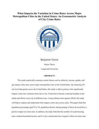
illustrated that population is not a main contributor to crime rates. A graph was created showing
each city’s population and its crime rates.

Figure 1. uses data gathered from the 252 US cities, and the crime rate as a
percentage for these cities. As Figure 1. shows, there is no significant relationship between the
population size of a city and its crime rate. This graph illustrates that there may be other factors
that play a much larger role in why crime rates vary from city to city. As seen in Figure 1,
Chicago, which is known for notoriously high murder rates has a crime rate that is around the
average for metropolitan cites. While this graph demonstrates that Chicago has a lower overall
crime rate comparatively, violent crimes are grouped together with other crimes, such as
property. This is significant because many people associate crime with only violent offenses.
Chicago does in fact have the third highest murder rate in the nation, but it’s total crime rate is
lower than about half of the cities in the study.
0%
2%
4%
6%
8%
10%
12%
100000 200000 300000 400000 500000 600000 700000 800000 900000 1000000
Figure 1.
Crime Rate To Population
Crime Rate To Population

In the past decade, crime rates have fallen substantially. Looking even further back to
1990, it is seen that crime rates have fallen by as much as 45%. Although crime rates are falling,
the media continues to portray heightened levels of crime. This could be due to the fact that
violent crimes may be on the rise in comparison to other crimes, and the media shows the violent
offenses more often comparatively.
Figure 2. displays that crime rates in the United States have been on a massive decline in
the past decade. While the crime rates have been decreasing in general, the amount of which they
are decreasing vary by city substantially. Another factor to consider is that while crime rates
have been shrinking, the amount of people being incarcerated has been increasing each year. An
additional element is that there are areas where crime has been rising in certain large cities even
though there is an overall decrease throughout the country, and these are the cities in which the
variation of crime rates is most severe.

Crime rates vary from city to city seemingly independent from population size. By
looking at the statistics for the whole country, variations between cities and states are made more
clear due to their lateral placement. When viewing these statistics, it is evident that variation
occurs substantially by states that are next to each other. This shows that the change can be
impacted by factors such as laws, and whether the state is liberal or conservative. While this
research deals specifically with cities, it is important to look at the amount of state funding that is
given for these expenditures, as well as the political affiliation of the states.
Figure 3. displays the violent crime indexes by state. One theory that is potentially dispelled is
that population size is a key contributing factor for crime rates. Based on the graph above, it
appears that there are some extreme differences between crime rates and population sizes. This is
Figure 2.

seen in Tennessee, which has a very high crime rate, and New York, which has substantially
lower crime rates, but a larger population. This large variation in crime rates will be reviewed by
comparing the cities regulations and laws among other factors.
There is evidence that there is a significant relationship between education, race, and crime.
Figure 4. shows the risk of imprisonment based on education and race over different time
periods. While this does not illustrate crime rates, it does show that there is a positive
relationship between education and those who are not as educated, regardless of race. The risk of
imprisonment may show that there is a relationship between being at risk for and subsequently
Figure 3.

committing a crime. The comparison of race to crime rate can be used to recreate the crime rates
in each individual city as this graph is an overall view of the United States.
Figure 4.

III. Literature Review
Shihadeh and Flynn (1996) explored the effect of segregation and the rates of black urban
violence. This study looked at urban indicators and race and looked at which population is more
affected by violent crime rates. They examined violent crime rates in one example, and found
that about 50 percent of all black urban males were arrested for a violent crime compared to
white urban males at 14%. This study specifically explores the impact of black isolation from
whites and how crime rates are affected in turn. In order to study this, they used an indicator of
black isolation from other ethnic groups, and different measures to show racially biased
predictors. They studied 151 United States cities with populations of over 100,000 and also had
at least 5,000 blacks living in the city. This study uses variables such as education, age,
population size, vacant housing, and the proportion of city officials who are black. Using this
data, they are able to show that urban blacks commit a higher rate of crime than urban whites. In
addition to this, they found that segregation varied significantly by city, where some cities would
have around 75 percent of black isolation. The study finds that there is significance between
segregation being a predictor for violent crime rates.
Blumstein and Wallman (2005) explored the changing rates of violence in the United
States from 1980-2000. The authors examined the impact of age on crime rates throughout cities
in the United States. The study found that as age increased, the number of murders committed by
that age group decreased. The study found that there was a much higher probability of an 18-
year-old male committing a crime than a 30-year-old male. This study encountered a few
limitations that may affect the importance of age on crime rates. One of theories that the author
mentioned was how younger offenders are more likely to be arrested possibly due to their lack of

experience in committing a crime. Using arrest rates, age, and police expenditures they compare
the rate of crimes committed between differing age groups across U.S cities. The results showed
that the younger the age, up until age 18, the more likely a violent crime is to be committed and
subsequently the offender has a higher chance of being arrested the younger they are. While this
study was important in showing that age is a fairly useful indicator for crime rates, if it is used in
addition to more predictors, age may help explain the variation in crime rates per city.
McDowall and Loftin (2009) confirm the generally accepted relationship that crime rates
in United States cities, follow a national to local trend covering 1940 to 2004. They use a
uniform system in order to insure that the cities they use are considered large metropolitan cities.
In order to keep this uniformity, they require the samples to keep a population size of over
100,000 for more than 30 years to insure they are among the United States most populous areas.
Their work delves into the post 1990 decrease in United States crime rates and crime trends on
both the national and local level. Their work was done to show that there were variations
between national data and local level date in regards to crime rates. Using data from cities over a
period of time, they attempt to identify the association between local and national crime trends.
One of the issues that the authors encountered was an aggregation issue, in which “long-term US
crime rate trends might not match trends in any of the nation’s cities” (McDowall 309). This
aggregation leads to the strength in which city crime rates mirror national ones. The study uses
homicide, rape, robbery, aggravated assault, burglary, larceny, and motor vehicle theft. Using
this data, they use counts for each offense, and compare them to the populations to get the rate of
crime. The regression results, with crime rate change in a given city as the dependent variable
show that a national pattern is followed by city level trends. They found that there is a is a fairly
strong relationship between local and national crime rates.

Ousey and Kubrin (2009) examined the effect that immigration had on crime rates on a
macro level. They studied 159 cities from 1980-2000 to see the widespread effect that
immigration has on crime rates over time. In their work, they wish to examine several
assumptions that are made in regards to immigration, and see how much is a fallacy of media,
and what is actually truth. Their research delves into formal social control, and immigration
selection effects. Immigrant selection effect states that as immigration over time increases, their
contribution to crime will fall. Formal social control means that stereotypes about immigrants
being criminals will lead to more fear among the public sphere, and as a result lead to laws about
immigrant and crime. They wished to use these theories to prove that immigration is not actually
a positive effect on crime, but rather that immigration leads to no change in crime rates or
possibly even lower crime rates. In order to prove that immigration doesn’t positively affect
crime rates, they used the violent crime rate as the dependent variable. In addition to this, they
used explanatory variables such as percentage of the population made up of foreign born persons
who immigrated in the past ten years, percentage of population that speaks English not well or
not at all, and percent Latino among other variables. This study used many of the same variables
to capture crime rates, but it’s inclusion of the immigrant population led to results that contradict
the overall assumption on immigration. Their study showed that immigration does not have a
positive effect on crime rates and that immigration in fact decreased levels of crime. This study
is something that will be used in research when determining crime rates, In addition, the percent
of the population that is of immigrant status will be added to see the effect on crime rates in
cities with differing immigration levels.
Hipp and Roussell (2013) investigate the micro and macro environment and the
consequences for crime rates. This study looks into the independent effects of population size

and density and how to distinguish them. Hipp and Roussel, propose that one explanation to
solve the problem with population density is to explore it from the micro-population density.
They use density exposure to capture the micro level, and measure the population within a
twenty-mile radius of the city in order to capture macro density. By doing this, they are able to
account for whether an area is surrounded by other cities, or whether it has low population levels
outside of the cities boundaries. Using crime data from all cities in the United States, they
compare the crime levels between the micro and macro population density levels. The regression
results with the type of crime as the dependent variable show that the biggest effect for robberies
and motor vehicles was higher in low density areas. In addition to this, robbery and homicide
showed that as population density started to increase, the number of violent crimes started to
occur more frequently. They also find that there is a fairly strong nonlinear relationship between
population density, population size, and crime. Within this data, the macro populations results
were significantly different from the micro level, suggesting that population size is not the main
indicator, but rather the population’s density level.

IV. Methodology
This empirical research is formatted using a cross sectional data set with explanatory
variables that will help to predict why crime rates vary for different metropolitan cities across the
United States. The data is from the year 2012 and represents cities with populations over
100,000. The large population size is typically an indicator for whether the size of a city, and as
such cities with populations under 100,000 will be omitted. Regression analysis will be used in
order to determine significance in the explanatory variables. For this study, Ordinary Least
Squares (OLS) will be used to run the regression. The model for why crime rates vary across
different cities can be seen below.
Model:
CrimeRatesi = β1 + β2Pop20-24i + β3Pop25-34i + β4Pop35-44i + β5DivRatei + β6Immigranti +
β7Unemploy + β8VacRatei + β9Democrati + β10Climatei + β11PopDensityi + β12Blacki +
β13Asiani + β14Hispanici + β15MedHouInci + β16HSGradi + β17ColGradi + β18MedHouVali +
β19MedRenti + εi
For the regression model, the dependent variable is the crime rate in cities with
populations over 100,000. The dependent variable was collected from the crime statistics study
conducted by the Federal Bureau of Investigation in 2012. It is conducted by taking the number
of crimes committed divided by the population of each individual city. For example, Chicago has
a population of 2.7 million and the number of crimes committed in Chicago was 96,016. Taking
theses two numbers and dividing them gives an overall crime rate of 4 percent or for every 1,000
people, four crimes are committed. Many studies have been conducted on violent crime rates
across the United States. This study will differ from other studies because it is viewing the total
crime rate variation across major metropolitan areas. Table 1. Illustrates variables that will be
used in the regression analysis and the expected signs that these variables are predicted to have

on crime rate variation across the United States. This data was collected from two separate
sources. The dependent variable, crime rates was obtained from the FBI data base, and the
explanatory variables were gathered from the United States Census Bureu.
Table 1.
Variable Name Definition Expected Sign Hypothesis Test
Ratesi
(Dependent
Variable)
The crime rate for each cityi
measured in %
------- ------
Blacki % of population that is Black,
in cityi
? Ho: = 0
HA: ≠ 0
Asiani % of population that is Asian
in cityi
? Ho: = 0
HA: ≠ 0
Hispanici % of population that is
Hispanic in cityi
? Ho: = 0
HA: ≠ 0
Pop20-24i % of population that is male
and aged 20-24 in cityi
+ Ho: ≤ 0
HA: > 0
+ Ho: ≤ 0
HA: > 0
- Ho: ≥ 0
HA: < 0
Divratei The average divorce rate for
cityi
+ Ho: ≤ 0
HA: > 0
Immigranti Percentage of cities
population that is comprised
of legal immigrants in cityi
- Ho: ≥ 0
HA: < 0
Unemployi % of population that is
unemployed in cityi
+ Ho: ≤ 0
HA: > 0
VacRatei % of home vacancy rates in
cityi
? Ho: = 0
HA: ≠ 0
MedHouInci The median household
income in cityi
? Ho: = 0
HA: ≠ 0
Democrati Dummy = 1 if city is
Democratic
? Ho: = 0
HA: ≠ 0
Climatei The average temperature for
cityi
+ Ho: ≤ 0
HA: > 0
HSGradi % of population who
graduated HS in cityi
- Ho: ≥ 0
HA: < 0
CollGradi % of population who
graduated college in cityi
- Ho: ≥ 0
HA: < 0

MedHouVali The average housing value for
cityi
- Ho: ≥ 0
HA: < 0
MedRent The average cost of rent in
cityi
- Ho: ≥ 0
HA: < 0
PopDen The population density for
cityi
+ Ho: ≤ 0
HA: > 0
Independent Variables:
Ethnicity
When holding all else constant, the effect of having minorities (Black, Hispanic, Asian)
in a city will impact crime rates, but it is unknown as to whether the crime rates will be affected
positively or negatively. While the expected sign is unknown, there is reason to believe that race
is an important variable when comparing crime rates. When looking at those imprisoned, the
percentage of blacks in jail greatly outnumbers whites, but there is no indication that blacks
commit more crimes.
Population Density
Population density is expected to have a positive effect on crime rates. This is due to the
fact that holding all else constant, areas with high population density offers opportunities for
more crimes to occur due to a larger population in a smaller, more confined area.
Percent Aged 20-24, 25-34, 35-44
As the percentage of the population that is male gets older, the crime rates are expected to
fall (Pop20-24,25-34,35-44). This means that holding all else constant, an increase in percent of
male population aged 20-24 and 25-34 will lead to an increase in crime rates. On the other hand,
as the percentage of the population that is male aged 35-44 increases, crime rates will decrease.
This is due to the fact that on average men commit more crimes than women, and younger
offenders are more likely to commit crimes and be caught for them.

Percent High School and College Grad
The average education level for each city (HS Grad, CollGradi) is expected to have a
negative sign. Holding all else constant, as the education level in a city decreases, it is expected
that crime rates will increase. People who have higher levels of education are less likely to
commit crimes because they may understand the consequences of their actions better than those
who are less educated.
Vacancy Rate
When holding all else constant, the expected sign on the coefficient of vacancy rates
(VacRatei) is unknown. As the vacancy rate in a city increases, it is expected to have an impact
on crime rates. This can be attributed to the fact that areas with high levels of crime may have
higher vacancy rates because people feel unsafe living in that area or that areas that are vacant do
not have valuables inside of them causing things such as theft to fall.
Immigrant
The percentage of the population that is considered to be legal immigrants (Immigranti) is
expected to have a negative sign. This means that ceteris paribus, as the percentage of
immigrants in a city increases, crime rates are expected to fall. An explanation for this could be
that immigrants in the United States are on a work visa or something similar, and as such it is
possible that they will commit less crimes in fear of deportation.
Median Income
When holding all else constant, the median income in each city (Incomei) is expected to
have an unknown impact. This means that as the average income in a city falls, crime rates are
expected to be impacted but the result is unknown. Typically, lower income areas have higher
crime rates. This can be explained by individuals turning to crime such as robberies, to make up

for their lack of income. A counter claim to this argument is that lower income areas have to
hold more jobs and thus are unable to have enough time to commit a crime.
Divorce Rate
The percentage of the population that has been divorced (Divratei)j is expected to have a
positive sign on crime rates. This means that holding all other variables in the model constant,
cities with higher divorce rates are expected to have higher crime rates. The divorce rate is
something that could signal a broken home and on average are more likely to commit a violent
crime than someone who did not come from a divorced family.
Political Affiliation
When holding all else constant, the political affiliation of the mayor elected in each city
(Democrati) is expected to have an impact on crime rates, but the impact is unknown. The
political affiliation can impact things such as gun rights and expenditures on securities cameras
among other things.
Climate
When holding all else constant, the average temperature of a city (Climatei) is expected to
have a positive effect on crime rates. According to many different studies, areas that have higher
temperatures on average tend to have higher crime rates.
Median Rent
The median rent (MedRenti) of a city is expected to have a negative effect on crime rates.
This means that holding all other variables in the model constant, as the median rent increases,
crime rates will decrease. The reasoning behind this is that more expensive rentals are often
larger and more secure which may deter crime.
Percent Unemployed

When holding all else constant, percent of the population that is unemployed
(Unemployi) is expected to have a positive impact on crime rates. This means that as the percent
of the population is unemployed increases, crime rates will grow. The increase in crime rates can
be explained by those who are now jobless have more free time on their hands and are more
willing to commit a crime to provide for their family.
Median Housing Value
The median housing value is expected to have a negative impact on crime rates. This
means that holding all else constant, as median housing value increases, crime rates will fall in
cityi. An argument as to why housing value will impact crime rates is due to property taxes.
Property taxes help fund police and public safety. This means that areas with higher median
housing value will have police forces that are better funded and might have more resources at
their disposal to deter crime.

V. Results:
This empirical study is taking data from 251 major metropolitan U.S cities. Each city has
a population over 100,000 to ensure that they are considered a large enough demographic. In
addition to this, OLS was used to test the results of the model.
Descriptive Statistics:
Table 2 shows descriptive statistics for major metropolitan cities across the United States.
The data shows that on average, the male population aged 20-24 accounts for 7.9% of total male
population with a range of 4.1% to 20.2%, males aged 25-34 accounts for 13% of total male
population with a range of 6.8% to 17.1%, and males aged 35-44 accounts for 12.5% of total male
population with a range of 8.5% to 15.9%. In addition, divorce rates averaged 22.6% per city, but
varied tremendously with a minimum of 11.9% to a maximum of 30.5%. For each city, the average
unemployment rate was 9.7%.
Crime
Rate
(per
10,000)
Population
male 20-24
(%)
Population
male 25-34
(%)
Population
Male 35-44
(%)
Divorced
(%)
Unemployed
(%)
Mean 190.10 7.907 13.11 12.50 22.60 9.70
Std. Dev. 138.46 2.60 1.52 1.03 3.35 2.59
Min 12 4.1 6.8 8.5 11.9 4.3
Max 1270 20.2 17.1 15.9 30.5 18.5
Count 251 251 251 251 251 251
Table 2. Descriptive Statistics

In order to effectively study crime rates, ethnicity, population density, and educational
attainment were obtained. The results from Table 3 show that the percentage of those who were
foreign born and legally immigrated to the United States was, on average, 8.17% of the population
and ranged from 1.1% to 38.3%. The average population of blacks in cities was 122,358 with a
minimum of 179 and maximum of 3,436,346 people. In addition, the average high school
graduation rate of cities in the sample was 87.04% with a minimum of 64% graduating high school
and a maximum of 95.5% graduating high school. Colleges graduates experienced a much lower
graduation rate for these cities when compared to high school. The average percentage of the
population that was a college graduate was 27% with a minimum of 8% and a maximum of 58%.
This is an exceptionally large variation in college graduation rates and could have an impact on
crime rate variations. The population density per square mile featured staggering differences, with
an average density of 2495. The minimum population density was 522.7 and the maximum was
31,251. These large difference could reflect higher crime rates in areas with larger population
densities.
Immigrant
(%)
Black Asian Hispanic High
School
Grad
(%)
College
Grad
(%)
Population
Density
Mean 8.17 122358 46033 162452 87.04 27.08 2495.83
Std.
Dev.
6.61 314830 193437 554542 5.44 8.28 2395.2
Min 1.1 179 192 1046 64 12.2 522.7
Max 38.3 3436346 2078246 5900913 95.5 58.5 31251.4
Count 251 251 251 251 251 251 251

Table 4 focuses on the descriptive statistics for income, housing rates, temperature, and
whether the city is represented by a democratic representative or not. The results show that the
average vacancy rate is 11.72% with a minimum of 4.7% and maximum of 40.6%. The median
household income was $49,683 with a minimum of $34,374 and maximum of $90,149. The
median housing values had the largest variation among this grouping. It had an average of
$165,022 with a minimum of $82,000 and a maximum of $453,500. In addition, the cities political
representation showed that 33% of the cities examined were represented by democrats.
Vacant
Housing
Rate
Median
Housing
Income
Median
Rent
Median
Housing
Value
Political
Affiliation
(1=Democrat)
Average
Temperature
Mean 11.72 49683.5 821.36 165022 .334 58.71
Std.
Dev.
5.16 8839.9 156.46 63426.2 .473 8.26
Min 4.7 34374 486 82300 0 29.95
Max 40.6 90149 1518 453500 1 78.15
Count 251 251 251 251 251 251

Significant Variables:
The OLS regression, which can be seen in Table 5 resulted in an R2
of .32 and six
significant variables. The R2
means that 32 percent of the variation in crime rates is explained
within the model. The percent of the male population aged 25-34 was significant at the 1% level
and had a positive impact on crime rates (t= 3.80 > tc = 2.59). Holding all else constant, a 1
percent increase in male population aged 25-34 increases crime rates by 2.85 percent. This
variable was expected to have an unknown coefficient and thus a two-sided test was used.
The percentage of families that are currently divorced was significant at the 1% level, and
had a positive coefficient (t= 5.42 > tc = 2.59). This means that holding all else constant, a 1
percent increase in the divorce rate per city increases crime rates by 12.75. This variable was
expected to have a positive result, and the regression confirmed the direction of the coefficient.
If a city is considered democratic, it is significant at the 5 % level, and the crime rate is
expected to be 27.81 percent lower than a city that has a republican political leader (t = -2.04 > tc
= 1.97). This variable was expected to have an unknown sign, and thus a two-sided test was
used.
A thousand-dollar increase in median household income decreased crime rates by 4
percent and was significant at the 5% level (t= -2.03 > tc = 1.97). This variable was expected to
have an unknown sign and a two-sided test was used.
A one percent increase in housing vacancy rates resulted in a decrease in crime rates by
3.21 percent and was significant at the 10% level ( t= 1.83 > tc = 1.65) This variable was
expected to have an unknown sign and a two-sided test was used.

A one thousand-unit increase in the population density resulted in crime rates increasing
by .953 percent and was significant at the 10% level (t= 1.92 > tc =1.65). This variable was
expected to have a positive sign and the regression confirmed the direction of the coefficient.
Insignificant Variables:
While the significant results give insight into what affects the variation in crime rates
across cities, there were some variables that are heavily debated in the news that were not
deemed significant. Some of the prominent variables that were not significant in determining
crime rates were the percentage of immigrants, high school and college grad, percent
unemployed, and the percent of the population that is black. In recent news headlines, some
politicians have made the claim that not only are immigrants taking away jobs, but they are also
harming American citizens. The model suggests that the percentage of immigrants have little to
no impact on the crime rates in major metropolitan cities. Another variable that had surprising
results was the percentage of unemployment not having a significant impact on crime rates. It
has been argued that areas with higher levels of unemployment will have higher crime rates, but
the results from this model do not support that claim. In addition, high school and college
graduates had a negligible effect on crime rates, this is somewhat surprising because areas that
are typically considered lower education level areas seem to have more crime, but the results
suggest otherwise.

Variable Coefficient Standard
Error
T-Stat P>|t|
Population Aged 20-24 Male 4.06 3.97 1.02 .307
Population Aged 25-34 Male 22.85 6.017 3.80*** .000
Population Aged 35-44 Male 7.62 11.13 .68 .494
Total Percent Divorced 12.75 2.35 5.42*** .000
Percent Immigrant -.72 2.27 -.32 .751
Percent Unemployed -.92 3.34 -.27 .784
Vacant Housing Rate -3.21 1.83 -1.75* .081
Democrat -27.81 13.63 -2.04** .043
Average Temperature .89 2.20 .40 .686
Population Density .953 .529 1.92* .056
Black -.000 .000 -1.22 .224
Asian .0000 .0000 -.01 .990
Hispanic -.0003 .0000 -.97 .332
Median Household Income -4.0 1.7 -2.03** .043
High School Graduate -2.74 3.33 -.82 .413
College Graduate .485 1.51 .32 .749
Median Housing Value .0000 .0003 .11 .913
Median Rent .086 .133 .64 .521
Table 5. Results Section
N=251; R
2
=.32; Adj. R
2
=.30;***=significant at 1%; **=significant at 5%; *=significant at 10%

Diagnostic Tests:
After running the OLS regression, diagnostics tests had to be run to ensure that the model
was robust and not affected by omitted variable bias, heteroskedasticity, irrelevant variables, or
multicollinearity. To test for multicollinearity, the variance inflation test (VIF) was run. This
evaluates the amount of collinearity between explanatory variables. If a variable has
multicollinearity, it can affect the standard errors. Looking at Table 6, it can be seen that there is
some correlation for both Asian and Hispanic, but the variables are important to the regression
equation and thus were left in. It should be noted that the model does suffer from some
multicollinearity. After seeing the high VIF, a correlation test was run to see which variables were
correlated to each other. Based on the results from STATA, there was correlation of .7728 between
Asian and Black, .6841 between Hispanic and Black, and .9263 between Asian and Hispanic.
Based on the correlation results, it would appear that the multicollinearity could be nothing more
than a coincidence. (Please refer to Appendix B for Correlation results.)

Variable VIF 1/VIF Variable VIF 1/VIF
Asian 14.36 .070 Black 3.91 .256
Hispanic 10.43 .096 Population 19-
24
4.70 .213
Median Rent 8.69 .115 Average
Temperature
2.77 .361
Median
Household
Income
7.82 .128 Total Divorce 2.37 .422
Table 6. VIF Test

Median
Housing
Value
6.66 .150 Population 24-
34
2.33 .429
Immigrant 6.49 .154 Population %
male
2.15 .466
College Grad 5.88 .170 Unemployed 2.12 .471
High School
Grad
5.23 .191 Vacant
Housing
1.90 .527
Population
Density
4.70 .212 Political
Affiliation
1.61 .623
Mean VIF 5.13
Next, the test for heteroskedasticity was run. The model that is being used did suffer from
heteroskedasticity at the 90% confidence level, and in order to correct for this, the robust
command was used in STATA. The robust command is a programmer’s command that computes
a robust variance estimator based on a variable list of equation-level scores and a covariance
matrix.
Model for Heterskedasticity:
𝐻#: 𝐶𝑜𝑛𝑠𝑡𝑎𝑛𝑡 𝑣𝑎𝑟𝑖𝑎𝑛𝑐𝑒
𝐻0: 𝑁𝑜𝑛 − 𝑐𝑜𝑛𝑠𝑡𝑎𝑛𝑡 𝑣𝑎𝑟𝑖𝑎𝑛𝑐𝑒
𝑃𝑟𝑜𝑏 > 𝑐ℎ𝑖2 = 0.000
The F-Test was used to determine if any of the variables in the regression equation were
statistically significant. According to the STATA results, the F-critical score was .0000
indicating that there is at least one significant variable.
When running the original OLS test, there were a few variables that were deemed
irrelevant, or did not affect the regression output. These variables when removed did not change
the adjusted R2
indicating that they were not necessary to the regression equation that was being
used.
The final step to ensure that the results were still the best linear unbiased estimator or
BLUE, a Ramsey Reset Test was run to check for any omitted variables. As expected, the results
of the Ramsey Test showed that there were some omitted variables. Data that would have been

useful to the model, such as police expenditures and percentage of the city that is considered blue
collar, was unable to be found and is most likely the reason that there may be omitted variables.

Model 2
The second model being used in this study changes the dependent variable from crime rates to
murder rates. As stated earlier, there has been a large amount of media portraying increasing
crime rates. One of the most reported crimes in the past few years has been murders. By
incorporating murder rates as the dependent variable, is will be possible to see how a part of the
crime rates may differ from overall crime rates. This test will use the same independent variables
as the first model, and all appropriate tests will be run.
Methodology:
This empirical research is formatted using a cross sectional data set with explanatory
variables that will help to predict why crime rates vary for different metropolitan cities across the
United States. The data is from the year 2012 and represents cities with populations over
100,000. The large population size is typically an indicator for whether the size of a city, and as
such cities with populations under 100,000 will be omitted. Regression analysis will be used in
order to determine significance in the explanatory variables. For this study, Ordinary Least
Squares (OLS) will be used to run the regression. The model for why murder rates vary across
different cities can be seen below.
Model:
MurderRatei = β1 + β2Pop20-24i + β3Pop25-34i + β4Pop35-44i + β5DivRatei + β6Immigranti +
β7Unemploy + β8VacRatei + β9Democrati + β10Climatei + β11PopDensityi + β12Blacki +
β13Asiani + β14Hispanici + β15MedHouInci + β16HSGradi + β17ColGradi + β18MedHouVali +
β19MedRenti + εi
For the regression model, the dependent variable is the murder rate in cities with
populations over 100,000. The dependent variable was collected from the crime statistics study

conducted by the Federal Bureau of Investigation in 2012. It is conducted by taking the number
of murder committed divided by the population of each individual city and then multiplied by
100,000. Many studies have been conducted on violent crime rates across the United States. This
study will differ from other studies because it is viewing the murder rates across major
metropolitan areas.
Results Model 2
The results from Table 8 show that when changing the dependent variable to murder
rates, there were many more significant variables, and some of the variables that were significant
in the first model had stronger significance levels. This empirical study is taking data from 251
major metropolitan U.S cities. Each city has a population over 100,000 to ensure that they are
considered a large enough demographic. In addition to this, OLS was used to test the results of
the model. The R2
means that 44 percent of the variation in murder rates is explained within the
model.
Descriptive Statistics:
Murder rates varied from crime rates in quite a few ways. When looking at the
descriptive statistics in Table 7, the results show that the average murder rate per 100,000 people
is 4.48, with a range of 0 to 20.6. This means that results will have smaller coefficients, but the
magnitude will still be large due to the relatively small murder rates.

Descriptive Statistics Murder Rate Per 100,000
Mean 4.48
Std. Dev. 3.25
Min 0
Max 20.6
Count 235
Significant Variables:
The percent of the population aged 25-34 who are male was significant at the 1 percent
level and the results show that the variable had a positive impact on murder rates (t = 3.77 > tc =
2.59). This means that holding all else constant, a 1 percent increase in the male population aged
25-34 increased murder rates by .64.
The percent of the population that legally immigrated to the United States was significant
and negative at the 1 percent level (t = -4.46 > tc = 2.59).. This means that holding all else
constant, a 1 percent increase in immigrants decreased murder rates by .17.
The percent of the population that is unemployed was significant and positive at the 1
percent level (t = 5.40 > tc = 2.59).. When holding all else constant, a 1 percent increase in
unemployment in cityi increased murder rates by .55.

The number of the population that is black was significant and positive at the 10 percent
level (t = 1.66 > tc = 1.65). Ceteris paribus, a 10,000 person increase in the black population
increased murder rates by .02.
The median household income for a family in cityi was significant and negative at the 10
percent level (t = 1.87 > tc = 1.65). This means that a $1,000 increase in median household
income decreased murder rates by .1.
The percent of people who graduated from high school was significant and negative at
the 1 percent level (t = 2.81 > tc = 2.59). This means that when holding all other variables
constant, a 1 percent increase in high school graduates decreased murder rates by .18.
The median housing value in cityi was significant and negative at the 5 percent level (t =
2.37 > tc = 1.97). When holding all else constant, a $10,000 increase in median housing value
decreased crime rates by .154.
Insignificant Variables:
In this regression, the expected signs from the first model were used, and there were three
variables that were significant but had the wrong expected signs. It is important to note that these
signs were expected with crime rates as the dependent variable and as such were deemed
insignificant due to incorrect sign.
The percent of the population aged 20 to 24 who are male was significant at the the 1
percent level. The results showed that this variable had a negative impact on murder rates while a
positive sign was expected. This variable was expected to be positive due to studies that showed
that younger adults don’t fully understand the risks that they are taking when committing a
crime, and are more willing to commit a crime.

The percent of the population that graduated from college was significant at the 10%
level. The results showed that this variable had a positive impact on murder rates and a negative
sign was expected. It is not known why this sign had a positive effect on murder rates.
The median rent was significant and positive at the 1% level, but the sign was incorrect.
It was predicted that as the average rent increased, the area would be considered a more
luxurious place to be, and as such there would be less crimes.
While there were more significant variables in this model, there were variables that were
significant in the first model that were not significant in the second model. Total divorce which
was significant at the 1 percent level in model 1 is now insignificant. This is interesting due to
the fact that areas with higher levels of divorce had higher crime rates, but murder rates were not
impacted by divorce. This could be due to the fact the crime rate captures all crimes, and many
of the crimes committed are those of young adults acting out. In addition, the political affiliation
of the city does not impact murder rates. In the news recently, there have been many headlines
about politics and gun rights. With these results, political affiliation does not seem to impact
murder rates any differently across cities. Another variable which was expected to be significant
but was not for both crime and murder rates was the population density. It was expected that as
population density increased, murder rates would increase. This is due to the fact that it is
heavily reported that areas such as New York have high amounts of crime, but according to these
results the area does not appear to matter.

Table 8. Model 2 Regression
Variable Coefficient Standard
Error
T-Stat P>|t|
Population Aged 20-24 Male -.387 .11 -3.46*** .001
Population Aged 25-34 Male .643 .170 3.77*** .000
Population Aged 35-44 Male -.170 .260 -.65 .513
Total Percent Divorced -.067 .069 -.98 .329
Percent Immigrant -.294 .066 -4.46*** .000
Percent Unemployed .549 .102 5.40*** .000
Vacant Housing Rate -.022 .040 -.55 .586
Democrat -.613 .394 -1.56 .121
Average Temperature .013 .036 .36 .719
Population Density .000 .000 .63 .531
Black .023 .012 1.66* .098
Asian .027 .035 -.77 .442
Hispanic .004 .005 .48 .635
Median Household Income -.1 .054 -1.87** .063
High School Graduate -.176 .063 -2.81*** .005
College Graduate .070 .039 1.82* .070
Median Housing Value .154 .065 -2.37** .019
Median Rent .012 .004 3.66*** .000

N=251; R
2
=.32; Adj. R
2
=.30;***=significant at 1%; **=significant at 5%; *=significant at 10%

Diagnostics Test:
Model 2 had an average VIF of 5.19, indicating that there was some significant
multicollinearity. The two variables with the highest VIF score were Hispanic and Asian, both of
which were insignificant variables. These variables were left in the regression due to the fact that
the study wished to see which ethnicities have an impact on crime rates. In addition, the second
model suffered from heteroskedasticity and as a result of this, the command robust was added to
the regression to provide results that are not skewed by heteroskedasticity.
Model for Heterskedasticity:
𝐻;: 𝐶𝑜𝑛𝑠𝑡𝑎𝑛𝑡 𝑣𝑎𝑟𝑖𝑎𝑛𝑐𝑒
𝐻0: 𝑁𝑜𝑛 − 𝑐𝑜𝑛𝑠𝑡𝑎𝑛𝑡 𝑣𝑎𝑟𝑖𝑎𝑛𝑐𝑒
𝑃𝑟𝑜𝑏 > 𝑐ℎ𝑖2 = 0.000
Table 9. VIF Model 2
Variable VIF 1/VIF Variable VIF 1/VIF
Asian 14.58 .069 Black 4.14 .242
Hispanic 10.75 .093 Population 19-
24
3.51 .285
Median Rent 8.94 .111 Average
Temperature
2.53 .396
Median
Household
Income
7.71 .130 Total Divorce 2.23 .448
Median
Housing
Value
6.83 .146 Population 24-
34
2.47 .406
Immigrant 5.71 .175 Population 35-
44
2.78 .359
College Grad 5.28 .189 Unemployed 2.26 .442
High School
Grad
5.38 .186 Vacant
Housing
1.94 .515
Population
Density
4.83 .207 Political
Affiliation
1.57 .636
Mean VIF 5.19

VI. Conclusion
This study examines what impacts crime rate variations in 251 major U.S. metropolitan
cities. Characteristics such as ethnicity, age, median income, and education levels are used to
understand what impacts crime rates. Crime rates have been on a steady decline since the 1960’s,
but are the most reported news topic in the United States. Economic policies about gun laws and
length of time someone should spend in prison have been discussed amongst politicians for
years. In addition, many individuals look at crimes as a deterrent for where they would live. For
example, an area such as New Orleans which has a high crime rate may not attract as many
people due to the high amounts of crime. This study will be able to aid policymakers and
individuals in determining solutions to fighting crime and finding a safe area to live and raise a
family.
The data used in this research is cross sectional data gathered from the FBI and the U.S.
Census Bureau from the year 2012. The estimation technique that this study will use is Ordinary
Least Squares (OLS) and there are 251 observations which are defined as major metropolitan
cities in the United States. The dependent variable is crime rates for model one, and murder rates
for model two. Some of the important explanatory variables for model one that are important are
population aged 25 to 34, divorce rate, vacancy rate, political affiliation, population density, and
median household income. The important explanatory variables for model two are percent of the
population aged 18 to 25, percent of the population aged 25 to 34, immigrant, unemployment
rate, amount of the population that is black, median household income, high school and college
graduate, median housing value, and median rent. Immigration has been a topic of heated
discussion in recent political debates, and the study finds that immigration doesn’t have an effect

on crime rates, and has a negative effect on murder rates. In addition, there were some variables
that were insignificant that showed interesting results. For model one, the percentage of
unemployment not having a significant impact on crime rates. It has been argued that areas with
higher levels of unemployment will have higher crime rates, but the results from this model do
not support that claim. In addition, high school and college graduates had a negligible effect on
crime rates, this is somewhat surprising because areas that are typically considered lower
education level areas seem to have more crime, but the results suggest otherwise. For model two,
there were three variables that were significant, but had the incorrect estimated sign. These
variables were percent of the population aged 18 to 24, percent of college graduates, and the
median rent. A potential reason for these variables being insignificant is because the expected
signs were the same as crime rates and not adjusted. After examining the variables, both
population aged 18 to 24 and the median rent could be explained as both positive and negative
effects on murder rates, but there was no solid information on why an area with a higher percent
of the population having a college education would increase murder rates.
In this study, many topics that are being debated in the 2016 presidential debate have
been explored by this model. Thus, with the results that have been discovered, some potential
policy implications may arise. Since divorce plays a role in crime rates, it could be suggested that
counseling be offered for families considering divorce. This could allow for families to
potentially work out the problems they are facing and remain together. Even if this policy
resulted in divorce rates going down by one percent, there would be a substantial drop in the
crime rates. In addition, population density had a positive impact on crime rates. This means that
areas that have more people per square mile results in more crimes. Policy makers could decide
to offer tax incentive for families to move to areas that have lower population densities, which

will lower the population density. Finally, median household income has a negative effect on
crime rates. This means that as the average income increases, there are lower crime rates in those
cities. In order to help curb this, a policy that pays people who live in high risk areas might be
considered. This policy is not without some merit either, in 2010, Richmond, California elected
officials introduced a program that paid at risk criminals up to $1,000 a month not to commit
crimes. According to Aaron Davis of the Washington Post, “five years into Richmond’s
multimillion-dollar experiment, 84 of 88 young men who have participated in the program
remain alive, and 4 in 5 have not been suspected of another gun crime or suffered a bullet
wound” (Davis 2016). After this implementation and subsequent falling crime rates, Washington
D.C has voted to pass a bill which would also pay at risk people to not commit crimes.
Model two examined the same explanatory variables, but changed the dependent variable
to murder rates. Murder rates have been a topic of recent discussion, and have dominated news
headlines. Many presidential candidates have claimed that immigrants are harmful to the United
States because they harm its citizens. The results of this study show the percent of the population
that are considered immigrants have a negative impact on murder rates, meaning that as the
percent of the population that is considered immigrant increases, murder rates go down. With
these results, it could be advised that the programs that are in place for those immigrating to the
United States are actually quite effective and do not need to be changed, which would decrease
budget spending in the United States. In addition, as the percent of high school graduate’s rises,
murder rates decrease. It could be advised that policy makers put more money and time in
developing better teachers and programs for schools that have high dropout rates. By increasing
the percent of high school graduates, there could be a drop in murder rates in the United States.

While this study produced robust and significant results, there were a few areas of
weakness in the project. The first problem that was encountered was because of testing issues.
The model suffered from multicollinearity which was not solved for due to the need of both
variables Hispanic and Asian. The reason that these variables remained in the regression
equation is because the study explored what ethnicities play a role in crime and murder rates. In
addition, the model did suffer from heteroskedasticity but is was fixed by adding robust to the
regression. Data that would have been useful to the model, such as police expenditures and
percentage of the city that is considered blue and white collar was unable to be found and is most
likely the reason that there may be omitted variables.
Since this project was only a semester long study, there were certain things that were
unable to be accomplished. If there were more time, it would have been valuable to examine
crime and murder rates over time to see how they have from city to city across many years. In
addition, if police expenditure were able to be used, the study could examine how adjusted for
inflation, the amount of money a police department receives impacts the crime and murder rates.

SeniorSemFinalW:OAppendixYarow

Recommended

Recommended

More Related Content

What's hot

What's hot (18)

Viewers also liked

Viewers also liked (13)

Similar to SeniorSemFinalW:OAppendixYarow

Similar to SeniorSemFinalW:OAppendixYarow (20)

SeniorSemFinalW:OAppendixYarow