posted by Bhawna Bhardwaj.

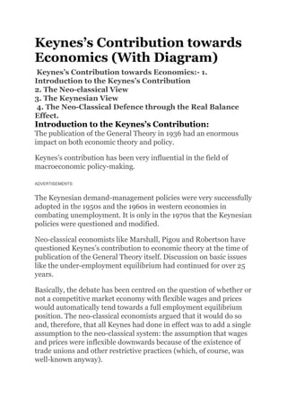
1. Keynes’s Contribution towards
Economics (With Diagram)
Keynes’s Contribution towards Economics:- 1.
Introduction to the Keynes’s Contribution
2. The Neo-classical View
3. The Keynesian View
4. The Neo-Classical Defence through the Real Balance
Effect.
Introduction to the Keynes’s Contribution:
The publication of the General Theory in 1936 had an enormous
impact on both economic theory and policy.
Keynes’s contribution has been very influential in the field of
macroeconomic policy-making.
ADVERTISEMENTS:
The Keynesian demand-management policies were very successfully
adopted in the 1950s and the 1960s in western economies in
combating unemployment. It is only in the 1970s that the Keynesian
policies were questioned and modified.
Neo-classical economists like Marshall, Pigou and Robertson have
questioned Keynes’s contribution to economic theory at the time of
publication of the General Theory itself. Discussion on basic issues
like the under-employment equilibrium had continued for over 25
years.
Basically, the debate has been centred on the question of whether or
not a competitive market economy with flexible wages and prices
would automatically tend towards a full employment equilibrium
position. The neo-classical economists argued that it would do so
and, therefore, that all Keynes had done in effect was to add a single
assumption to the neo-classical system: the assumption that wages
and prices were inflexible downwards because of the existence of
trade unions and other restrictive practices (which, of course, was
well-known anyway).

2. Keynesians, on the other hand, attempted to show that a
competitive economy, even with completely flexible wages and
prices, would not be likely to achieve full employment
automatically. Consider how this debate progressed.
The Neo-classical View:
The neo-classical view was that a perfectly competitive economy
would always tend towards its full employment equilibrium
position. This is illustrated in the three- graph diagram in Fig. 14.13.
The upper graph shows the economy’s initial general equilibrium
position in the real and monetary’ sectors.
ADVERTISEMENTS:
The lower left-hand graph is the short-run aggregate production
function and the lower right-hand graph illustrates the economy’s
labour market. Notice that for convenience the real wage is
measured along the horizontal axis and the quantity of labour is
measured along the vertical axis. As drawn, equilibrium in the real
and monetary sectors exists at an output level of OY1 which is
produced using a quantity of labour OL1. Unfortunately, this is not
the full employment quantity of labour: there is an excess supply of
labour (or unemployment) equal to BC.

3. According to the neo-classical economists, this unemployment
cannot persist. Assuming that wages and prices are flexible upwards
and downwards, the excess supply of labour will cause money wages
to fall. As the real wage falls, employment and output rise, but this
spoils the equilibrium in the real and monetary sectors of the
economy.
ADVERTISEMENTS:
In fact, there will be an excess supply of goods and services on the
market which will exert downward pressure on prices. The result,
then, is a general deflation of both wages and prices which leaves
real wages unchanged but which causes the real money supply to
increase, so shifting the LM curve to the right to LM’. This deflation,
according to the neo-classical economists, will continue until the
new equilibrium in the real and monetary sectors is just consistent
with equilibrium in the labour market-that is, at point A in Fig.
14.13. Only when this point is reached will the unemployment in the
economy have been eradicated.
The Keynesian View:
Keynesians were sceptical of the above mechanism, even assuming
flexible wages and prices. In particular, they pointed to two barriers
which might exist to prevent the full employment equilibrium from
being reached: lack of investment and the liquidity trap.
The possible lack of investment is illustrated in Fig. 14.14 where the
IS curve is very steep and cuts the horizontal axis at a point below
the full employment level of income Y1. Recall that the IS curve will
be steep when investment is very interest- inelastic. In this case, as
shown in the diagram, it is impossible for a full employment
equilibrium to be reached by means of a shifting LM curve alone.

4. Recall that it exists where the interest rate is so low that the demand
for money becomes perfectly interest-elastic. When the demand for
money is perfectly interest-elastic, the LM curve is horizontal, as
illustrated in Fig. 14.15.
In this ease, the equilibrium level of income is unaffected by the
increase in the real value of the money supply. The LM curve shifts
to the right, as shown, but the intersection of the horizontal part of
the LM curve with the IS curve is unchanged. What is happening
here is simply that the additional real money supply is being held in
speculative or ‘idle’ balances.
The Neo-Classical Defence through the Real Balance
Effect:
The neo-classical economists, largely through the work of Pigou,
produced a counter-argument to the above Keynesian cases in the
shape of the real balance effect. According to this, with a constant

5. nominal money supply, a general deflation of wages and prices will
tend to increase the real value of people’s holdings of money above
their desired levels.
Consequently, people will reduce their savings and increase their
consumption in an attempt to reduce their ‘real balances’. In the
above cases, where full employment is not reached, as wages and
prices fall and the LM curve shifts to the right, the IS curve will also
shift to the right as consumption increases. With both curves now
shifting to the right, the equilibrium levels of income and
employment must increase (even in the liquidity trap and with
interest-inelastic investment) and there is now nothing to stop full
employment from being reached. This is illustrated in Fig. 14.16.
Theoretically, then, the neo-classical economists appear to have the
stronger case. Only when it came to policy-making did the
Keynesians have the upper hand, given the recognised inflexibility
of wages and prices downwards.
Related Articles
Keynes’s Contribution to Economic Theory | Keynes’s General Theory
Keynes’s Liquidity – Preference Theory of Interest Rate
Keynes’s Criticism on Classical Theory of Market: 6 Criticisms | Say’s Law
by Taboola
Sponsored Links
You May Like
Represent the Future With IETCInfosys

6. Forbes' List of India's Richest PeopleForbes
Born between 1956 to 1996? You can earn a potential second income with
companies like Amazon CFDs!Capitalix
Goodbye Cell Phone, Hello VoIP (Find out Why Many are Switching to
VoIP)Low Cost VoIP Phone | Search AD
Goodbye Cell Phone, Hello VoIP. Why Everyone Is Switching To VoIPVoIP
Phone | Search Ads
Top 20 Of The Most Heavenly Beaches In The WorldBest-journal.xyz
Welcome to EconomicsDiscussion.net! Our mission is to provide an online platform to help students
to discuss anything and everything about Economics. This website includes study notes, research
papers, essays, articles and other allied information submitted by visitors like YOU.
Before publishing your Articles on this site, please read the following pages:
1. Content Guidelines
2. Privacy Policy
3. TOS
4. Disclaimer Copyright
Share Your KnowledgeShare Your Word FileShare Your PDF FileShare Your
PPT File
Sponsored Links
You May Like
Luxury Watches Are Sold for Almost Nothing - See Prices!Unsold Luxury Watches
Keynes’s Contribution towards
Economics (With Diagram)
Article Shared by
ADVERTISEMENTS:

7. Let us make an in-depth study of Keynes’s Contribution
towards Economics:- 1. Introduction to the Keynes’s
Contribution 2. The Neo-classical View 3. The Keynesian
View 4. The Neo-Classical Defence through the Real
Balance Effect.
Introduction to the Keynes’s Contribution:
The publication of the General Theory in 1936 had an enormous
impact on both economic theory and policy.
Keynes’s contribution has been very influential in the field of
macroeconomic policy-making.
ADVERTISEMENTS:
The Keynesian demand-management policies were very successfully
adopted in the 1950s and the 1960s in western economies in
combating unemployment. It is only in the 1970s that the Keynesian
policies were questioned and modified.
Neo-classical economists like Marshall, Pigou and Robertson have
questioned Keynes’s contribution to economic theory at the time of
publication of the General Theory itself. Discussion on basic issues
like the under-employment equilibrium had continued for over 25
years.
Basically, the debate has been centred on the question of whether or
not a competitive market economy with flexible wages and prices
would automatically tend towards a full employment equilibrium
position. The neo-classical economists argued that it would do so
and, therefore, that all Keynes had done in effect was to add a single
assumption to the neo-classical system: the assumption that wages
and prices were inflexible downwards because of the existence of
trade unions and other restrictive practices (which, of course, was
well-known anyway).
Keynesians, on the other hand, attempted to show that a
competitive economy, even with completely flexible wages and
prices, would not be likely to achieve full employment
automatically. Consider how this debate progressed.

8. The Neo-classical View:
The neo-classical view was that a perfectly competitive economy
would always tend towards its full employment equilibrium
position. This is illustrated in the three- graph diagram in Fig. 14.13.
The upper graph shows the economy’s initial general equilibrium
position in the real and monetary’ sectors.
ADVERTISEMENTS:
The lower left-hand graph is the short-run aggregate production
function and the lower right-hand graph illustrates the economy’s
labour market. Notice that for convenience the real wage is
measured along the horizontal axis and the quantity of labour is
measured along the vertical axis. As drawn, equilibrium in the real
and monetary sectors exists at an output level of OY1 which is
produced using a quantity of labour OL1. Unfortunately, this is not
the full employment quantity of labour: there is an excess supply of
labour (or unemployment) equal to BC.
According to the neo-classical economists, this unemployment
cannot persist. Assuming that wages and prices are flexible upwards
and downwards, the excess supply of labour will cause money wages
to fall. As the real wage falls, employment and output rise, but this

9. spoils the equilibrium in the real and monetary sectors of the
economy.
ADVERTISEMENTS:
In fact, there will be an excess supply of goods and services on the
market which will exert downward pressure on prices. The result,
then, is a general deflation of both wages and prices which leaves
real wages unchanged but which causes the real money supply to
increase, so shifting the LM curve to the right to LM’. This deflation,
according to the neo-classical economists, will continue until the
new equilibrium in the real and monetary sectors is just consistent
with equilibrium in the labour market-that is, at point A in Fig.
14.13. Only when this point is reached will the unemployment in the
economy have been eradicated.
The Keynesian View:
Keynesians were sceptical of the above mechanism, even assuming
flexible wages and prices. In particular, they pointed to two barriers
which might exist to prevent the full employment equilibrium from
being reached: lack of investment and the liquidity trap.
The possible lack of investment is illustrated in Fig. 14.14 where the
IS curve is very steep and cuts the horizontal axis at a point below
the full employment level of income Y1. Recall that the IS curve will
be steep when investment is very interest- inelastic. In this case, as
shown in the diagram, it is impossible for a full employment
equilibrium to be reached by means of a shifting LM curve alone.

10. Recall that it exists where the interest rate is so low that the demand
for money becomes perfectly interest-elastic. When the demand for
money is perfectly interest-elastic, the LM curve is horizontal, as
illustrated in Fig. 14.15.
In this ease, the equilibrium level of income is unaffected by the
increase in the real value of the money supply. The LM curve shifts
to the right, as shown, but the intersection of the horizontal part of
the LM curve with the IS curve is unchanged. What is happening
here is simply that the additional real money supply is being held in
speculative or ‘idle’ balances.
The Neo-Classical Defence through the Real Balance
Effect:
The neo-classical economists, largely through the work of Pigou,
produced a counter-argument to the above Keynesian cases in the
shape of the real balance effect. According to this, with a constant
nominal money supply, a general deflation of wages and prices will
tend to increase the real value of people’s holdings of money above
their desired levels.
Consequently, people will reduce their savings and increase their
consumption in an attempt to reduce their ‘real balances’. In the
above cases, where full employment is not reached, as wages and
prices fall and the LM curve shifts to the right, the IS curve will also
shift to the right as consumption increases. With both curves now
shifting to the right, the equilibrium levels of income and
employment must increase (even in the liquidity trap and with

11. interest-inelastic investment) and there is now nothing to stop full
employment from being reached. This is illustrated in Fig. 14.16.
Theoretically, then, the neo-classical economists appear to have the
stronger case. Only when it came to policy-making did the
Keynesians have the upper hand, given the recognised inflexibility
of wages and prices downwards.
Keynesian system involves six functional relations, viz.
consumption function (or the saving function), the investment
function, the demand function for money, aggregate production
function, the demand function for labour, and the supply function
of labour. Keynes’ saving function, money demand function, and
labour supply function are really different from that of the classical
system.
The primary determinant of Keynes’ saving function is income
rather than the classical rate of interest.
That is,
S = f (Y) …(10.24)
Keynes added the speculative demand for money, L(r), to classical
transaction demand for money, kPY.
Thus, Keynes’ money demand function is written as

12. M = kPY + L(r) …(10.25)
where speculative demand for money depends on the rate of
interest, r.
Keynes’ labour supply function is assumed to depend on money
wages which are institutionally rigid in the downward direction.
ADVERTISEMENTS:
Thus, labour supply function is
SL = f (W) …(10.26)
Where, W is the money wage.
However, the aggregate production function, investment function,
and labour demand function of Keynes do not differ from the
classical forms.
Keynesian income determination theory can explain
macroeconomic problems once we incorporate money market in
our analysis. It is the rate of interest, determined by the demand for
money and the supply of money that integrates goods market and
money market. Rate of interest not only influences investment but
also (speculative) demand for money.
Thus, a synthesis of income and monetary analysis is brought about
by the interest rate. Equilibrium national income is determined in
the goods market when saving, equals investment. Monetary
equilibrium is attained in the money market when demand for and
supply of money are equal to each other.
By establishing equilibrium in the goods market and money market,
equilibrium level of national income and the rate of interest are
simultaneously determined.
To establish ‘general equilibrium’, we use the Hicks- Hansen
tool, most popularly known as the IS- LM tool. The IS-LM analysis,
a neo-Keynesian analysis, explains Keynesian macroeconomic

13. system that takes into account goods market and money market
simultaneously.
Goods Market Equilibrium: The IS Curve:
Keynesian theory of aggregate demand is inadequate to explain
macroeconomic system when the money market is introduced. So,
we need to establish a link between the money market and the
goods market through the rate of interest. Now, we treat interest
rate as a variable whose equilibrium value is determined
simultaneously with that of the level of income.
ADVERTISEMENTS:
In the goods market, we have:
(a) The saving function
(b) The investment function
(c) An equilibrium condition.
ADVERTISEMENTS:
These are expressed as:
S = f (Y) …(10.24)
I =f (r) …(10.14)
and S = I …(10.27)
ADVERTISEMENTS:
To develop the IS curve our task is to find combinations of interest
rate, r, and the level of income, Y, that equate investment with
saving. We cannot solve equation (10.27) for Y to determine
equilibrium Y, unless we know Y. If ‘r’ is unknown, we cannot find
out the volume of investment expenditure. At a given ‘r’, one can
determine the volume of investment expenditure.
Once we determine investment expenditure, we are able to find out
the equality between investment and saving. Consequently,
equilibrium national income is determined in the goods market. In

14. fact, there are a series of combinations of r and Y that ensure
equality between saving and investment.
Once these combinations are plotted on the r – Y plane, we get a
curve which Hicks-Hansen called the IS curve. The IS curve shows
alternative combinations of national income (Y) and the rate of
interest (r) which equilibrate the commodity market.
Mathematically, the IS curve is simply the solution of equation
(10.27) for r in terms of Y.
Fig. 10.27 illustrates the construction of the IS curve. In the upper
panel of the figure, we have drawn the aggregate expenditure (C + I)
schedule. National income is determined at that point where the
aggregate demand line cuts the 45° line. We start with the given rate
of interest.
Suppose, the initial rate of interest is r0. At this rate of interest,
aggregate demand schedule, C + I (r0), cuts the 45° line at E. The
corresponding level of income is YQ. As investment is inversely
related to the interest rate, decrease in the interest rate from r0 to r,

15. causes investment to rise. Consequently, aggregate demand line
shifts up to C + I (r1).
ADVERTISEMENTS:
The new aggregate expenditure schedule cuts the 45° line at E1 and
the corresponding level of national income rises to Yr Thus, for the
interest rate r0, a point of product market equilibrium will be Y0.
This r0 – Y0 combination is one point on the IS curve, shown in the
lower panel of Fig. 10.27. Similarly, r1 interest rate produces
Y1 equilibrium income. So, r1 — Y1 combination is another point on
the IS curve. By joining these points we get a curve known as the IS
curve.
Thus, the IS curve is the locus of all equilibrium combinations of r
and Y that bring product market in equilibrium.
Any point off the IS curve shows disequilibrium in the goods
market. To the right of the IS curve, there occurs excess supply of
goods (ESG) when aggregate output exceeds aggregate demand, i.e.,
Y > C + I. To the left of the IS curve there arises excess demand for
goods (EDG) when aggregate demand exceeds aggregate output,
i.e., C + I > Y.
Thus the effect of an increase in r is:
r ↑→ I↓→ AD ↓→Y↓, and the effect of a fall in r is:
ADVERTISEMENTS:
r ↓→ I ↑→ AD↑→ Y↑
The IS curve slopes downwards to the right. Or it has a negative
slope.
Its slope depends on the saving function and investment function.
The IS curve will be relatively steep (flat) if investment is less
(more) sensitive to interest rate changes. The IS curve will be
vertical if investment is absolutely interest-inelastic. An
autonomous increase in investment expenditure or government
expenditure will shift the IS curve to the right.

16. (a) Alternative Method of Deriving the IS Curve:
The derivation of IS curve can be made in terms of the four-part
diagram (Fig. 10.28). In part (a), we have drawn investment
function that shows the inverse relationship between investment
and the rate of interest. Part (c) plots the saving function that
represents direct relationship between income and saving. Part (b)
is simply a 45° identity line, and part (d) plots the IS curve.
Suppose the rate of interest is r0. At this rate of interest, investment
must be I0 and, thus, the volume of saving must be S0, necessary for
equilibrium. This volume of saving implies an equilibrium income
of Y0 necessary for equilibrium. This establishes one point on part
(d), say point M. If the rate of interest rises to r1; investment declines
to I1. This results in a decline in national income to Y1.
ADVERTISEMENTS:
With this level of income the volume of saving becomes S1. This
establishes another point on part (d), say point N. The procedure
may be repeated for each level of income (interest) to obtain
corresponding values of interest rate (income value) that ensure

17. equality between saving and investment. By joining all these
equilibrium points we get an IS curve drawn in part (d).
Thus, the IS curve shows various combinations of income and
interest rate that brings the commodity market in equilibrium. The
IS curve is negatively sloped. Its slope depends on the nature of
saving and investment functions.
The IS curve may shift if there is a change in autonomous private
investment and government expenditure.
Properties of the IS Curve: A Summary:
i. The IS curve is the equilibrium combinations of income and
interest rate such that the product market or goods market is in
equilibrium.
ii. The IS curve slopes downward to the right because an increase in
interest rate causes investment expenditure to decline, therefore,
reduces aggregate demand and, hence, equilibrium national
income.
ADVERTISEMENTS:
iii. Its slope depends on the saving and investment functions. The IS
curve will be relatively steep (flat) if investment is less (more)
sensitive to interest rate changes.
iv. This IS curve will shift by an autonomous change in investment
spending or government spending.
v. Any point on the IS curve shows that there is neither excess
supply nor excess demand for goods. Any point off the IS curve
shows either excess supply of goods (ESG) or excess demand for
goods (EDG).
Money Market Equilibrium: The LM Curve:
Equilibrium in the money market occurs at that point where money
demand equals money supply. In the Keynesian system, money
demand for transaction purposes depends on the level of income
and money demand tor speculative purposes depends on the rate of
interest.

18. Thus, the money demand function, denoted by Md, can be
expressed as:
Md = f(Y, r) …(10.28)
Supply of money (M) is institutionally given. Given M,
corresponding to each level of income there is a rate of interest
which produces equilibrium in the money market. Money market
equilibrium occurs when
M = Md …(10.30)
The LM curve shows different combinations of r and Y that
equilibrate money market. In Fig. 10.29 we have drawn two money
demand schedules, corresponding to two different levels of income.
At Y0 income, money demand schedule is given by Md (Y0). As
income increases from Y0 to Y1, the money demand curve shifts to
the right. The vertical line M shows fixed money supply.
We find equilibrium in the money market when money demand
schedule intersects money supply schedule.
We start with a given income, Y0. At Y0 level of income, money
demand schedule is Md (Y0). The rate of interest is r0. As income
rises to Y1, money demand schedule shifts to Md(Y1) and the rate of
interest rises to r1. Thus, we find a direct relation between money
demand and interest rate at different levels of income.
The effect of an increase in Y is:
Y ↑→ Md↑→ r↑ and the effect of a fall in Y is:
Y↓→Md ↓→r ↓.

19. The interest-income combination at which equilibrium occurs, (r0 –
Y0) and (r1 – Y1), are points along the LM curve. These points are
plotted in Fig. 10.30. Thus, the LM curve is the locus of all
combinations of r and Y that bring money market in equilibrium.
This LM curve slopes upward to the right because as interest rate
rises equilibrium income rises. The slope of the LM curve depends
on the interest elasticity of money demand. If interest elasticity of
money demand is interest-inelastic the LM curve will be steep and if
money demand is assumed to be highly interest-elastic, the LM
curve will be flatter.
In an extreme case, if money demand is assumed to be perfectly
interest-elastic (it happens at the floor rate of interest or the so-
called liquidity trap region) the LM curve becomes perfectly elastic
at this region. In Fig. 10.30 the LM curve is drawn parallel to the
horizontal axis at the minimum rate of interest, rmin. The LM curve
becomes positively sloped above the rmin range.
Any point off the LM curve shows disequilibrium in the money
market. Just to the right of the LM curve there arises excess
demand for money (EDM) and to the left of the LM curve excess
supply of money (ESM) arises.
(a) Alternative Method of Deriving the LM Curve:
A four-part diagram may be used to derive the LM curve. Fig.
10.29(a) shows a proportional relationship between money income
and transaction demand for money (Mt = kPY). Part (c) represents
speculative demand for money [MS = fir)]. The schedule in (b) is an

20. identity line that mechanically divides money supply into
transaction and speculative elements. Part (d) represents the LM
curve.
Suppose, rate of interest, r0, is known. Given r0, the volume of
speculative demand for money is MS0. Given the total money supply
(M), money not used for speculative purposes must be held for
meeting transaction demand for money. Thus, the transaction
demand must be Mt0. To ensure this transaction demand for money
there must be a level of income Y0.
Thus, we see in part (d), for interest rate r0, the only possible money
market equilibrium value for income is Y0. If the rate of interest
declines to r0, the equilibrium level of income will be Y1. The
procedure can be repeated such that equilibrium combinations of r
and Y emerge to ensure equality in the money market.
By joining all these combinations (M and N), we get the LM curve
drawn in part (d). Note that at a floor interest rate, rmin, money
demand becomes infinitely elastic. This makes speculative demand
for money (shown in part c) to become horizontal at the minimum
rate of interest. Because of this liquidity trap, the LM curve also
becomes perfectly elastic. Anyway, the LM curve slopes upward
from left to right.

21. Properties of the LM Curve: A Summary:
i. The LM curve consists of equilibrium combinations of income and
interest rate for the money market.
ii. The LM curve slopes upward to the right.
iii. The slope of the LM curve depends on the interest elasticity of
money demand. The LM curve will be (flat) steep if the interest-
elasticity of money demand is relatively (low) high.
iv. The LM curve shifts due to changes in money supply and money
demand.
v. All points on the LM curve show money market equilibrium such
that there is neither excess demand for money (EDM) nor excess
supply of money (ESM). Any point off the LM curve exhibits either
EDM or ESM.
Combining Goods Market and Money Market:
General Equilibrium:
Goods market and money market do not operate independently—
one influences the other. Thus, combining these two markets, we
can determine the values of Y and r that are consistent with
equilibrium in these two markets.
The interrelationships or the links between these two
markets are:
There is a link between investment and interest rate determined in
both the goods market and money market. Investment here is
assumed to be determined by the interest in a negative fashion. We
have amply demonstrated here that the interest rate is determined
in the money market. Thus, money market influences goods market.
Another link can be traced between output/income and demand for
money. We have seen that aggregate output determined in the
goods market influences demand for money. An increase in income
(keeping interest rate constant) causes an increase in money
demand.
These two links can be shown in the following form:

22. Fig. 10.32 shows the general equilibrium in terms of IS and LM
curves. Here, when both the curves are plotted on the same axes,
the equilibrium level of income, Ye, and the equilibrium interest
rate, re, are determined simultaneously.
This is known as the synthesis of monetary analysis and income
analysis or macroeconomic general equilibrium. Point E is the
(only) point of general equilibrium for both the markets. Point E is a
stable equilibrium point.
To demonstrate stability, let us consider r1 – Y1 combination. Since
this combination is on the IS curve, the product market is in
equilibrium while money market is not. At this combination, there
is an excess demand for money (EDM). To meet this excess
demand, people will go on selling bonds.
This will depress bond prices and raise interest. As interest rate
increases, there are repercussions in the product market. Now,
following an increase in interest rate, investment declines and, as a
consequence, income declines. So, interest rate and national income
will go on changing until point E is reached, if the equilibrium is to
be a stable one. This occurs only at re and Ye.

23. Similarly, any r – Y combination above re will exhibit equilibrium in
the money market, but disequilibrium in the product market. Now,
product market will experience a deficiency in aggregate demand.
This causes income to decline. As income declines, there are
repercussions in the money market. Now, demand for money will
decline as income declines. So, rate of interest must decline. If
equilibrium is stable, r and Y tend to change until point E is
reached. Thus, E is a stable equilibrium point.
One thing should be borne in mind—to have stability in
equilibrium, the slope of the IS curve should be less than that of the
LM curve.
Shifts of the IS and LM Curves: Effects of Fiscal and
Monetary Policy Change:
It may be noted that the fiscal policy change (a change in taxes or
government expenditures) will shift the IS curve, and monetary
policy change will shift the LM curve.
(a) Monetary Policy:
Monetary policy attempts to stabilize the aggregate demand in the
economy by regulating the money supply. An expansionary
monetary policy is needed to stimulate the economy. This makes the
LM curve to shift to the rightward direction. Note that, in Fig. 10.33,
we have drawn negative sloping IS curve and positive sloping LM
curve.
The LM curve has three stages:

24. (i) Liquidity trap region where the LM curve is horizontal (also
known as the Keynesian region)
(ii) The classical region where the LM curve is vertical, or perfectly
inelastic, and
(iii) The intermediate region where the LM curve is positively
sloped.
In the liquidity trap region or extreme Keynesian range, monetary
policy is totally ineffective in stimulating income. Despite an
increase in money supply, LM curve does not change its position.
An increase in money supply cannot cause the interest rate to fall
below the rate given by the liquidity trap. Equilibrium income then
remains unchanged at OY0.
As was believed by Keynes during the Great Depression years of the
1930s that the economy was caught in the trap region then he
recommended for the use of unorthodox fiscal policy. In other
words, monetary policy was to be discarded during the early 1930s
as it would be grossly ineffective in stimulating the economy.
The essence of the argument is that since government is helpless in
raising income/output level through monetary policy, the
government has to employ the fiscal policy. Anyway, it must be said
that the liquidity trap is an extreme case.
Secondly, in the classical region, where the LM curve is vertical,
monetary policy becomes completely effective. As the LM curve
shifts to LM1; rate of interest declines more this time from Or4 to Or3.
This causes income to rise by a larger amount from OY3 to OY4. In
view of this, classicists favour monetary policy.
But Keynesians reject monetary policy during depression when the
rate of interest reaches a floor level. Thus, in the classical range,
monetary policy is completely effective in contrast to the Keynesian
or liquidity trap region in which monetary policy is totally
ineffective, (i.e., the LM curve is perfectly elastic).
Finally, in the intermediate range where the LM curve is positive
sloping, an increase in money supply shifts the LM curve from LM

25. to LM1. Consequently, interest rate declines to Or1 and income rises
from OY1 to OY2, Thus, monetary policy is effective.
To be more specific, monetary policy is found to have a degree of
effectiveness but not the complete effectiveness as we see in the
classical region. In general, the closer the equilibrium (of IS and LM
curves) is to the classical region, the more effective monetary policy
becomes, and the closer the equilibrium is to the Keynesian range,
the less effective monetary policy becomes.
(b) Fiscal Policy:
Fiscal policy also attempts to influence aggregate demand in an
economy by influencing tax-expenditure programme of the
government. A cut in taxes or an increase in government spending
causes a shift in the IS curve in the rightward direction.
In Fig. 10.34, the IS curve intersects the LM curve at its horizontal
portion (i.e., liquidity trap region). In this region, as the IS curve
shifts from IS to IS1, the equilibrium level of income rises from
OY0 to OY1. Thus, fiscal policy is completely effective in stimulating
aggregate income in the depressionary phase without having any
effect on interest rate.
Secondly, in the classical range, fiscal policy is completely
ineffective since it fails to stimulate aggregate demand and, hence,
aggregate income. Fig. 10.34 says that the increased government
expenditure and/or decreased taxes shifts the IS curve in the clas-
sical region (where the LM curve is vertical) from IS4 to IS5.

26. This causes equilibrium intersection to shift up. This results in an
increase in the interest rate only from Or3 to Or4, keeping income
level unchanged at OY4.
Finally, fiscal policy is partly effective in the normal intermediate
range where both interest rate and income rise. Fiscal measures
that shift the IS curve from IS2 to IS3, in the section between
Keynesian and classical section, called, intermediate section, raises
the level of income from OY2 to OY3 and the rate of interest from
Or1 to Or2.
Thus, fiscal policy is found to have a degree of effectiveness in this
region. It may be concluded that, in general, fiscal policy becomes
more effective the closer the IS-LM intersection or equilibrium lies
to the Keynesian or liquidity trap region and less effective the closer
the equilibrium point resides to the classical region.
Thus, fiscal policy may be employed in depression years. This is the
Keynesian argument. It is argued that these results concerning
monetary policy are the opposites of the results obtained under
fiscal policy regime.
Thus, one can conclude that the effectiveness of monetary
policy depends on:
(i) The interest-elasticity of the demand for money, and
(ii) The interest elasticity of investment. These two aspects can be
illustrated in terms of Fig 10.35.
If the LM curve is vertical (pure classical case), monetary policy
becomes highly effective in raising equilibrium income [Fig.
10.35(a)]. Consequent upon an increase in money supply, the LM
curve shifts from LM to LM1. Equilibrium interest rate now declines
from Or1 to Or2 and equilibrium income rises from OY1 to OY2.
The biggest effect of monetary policy can be felt if the IS curve is
perfectly elastic [Fig. 10.35(b)], Note that, following a shift in the
LM curve from LM to LM1, national income rises from OY: to
OY2 without influencing the interest rate that remains at Or1.
On the other hand, if the LM curve is horizontal (pure Keynesian
range) and if the IS curve is vertical, monetary policy becomes
ineffective completely [Figs. 10.35(c) and (d)]. Fig. 10.35(c) says

27. that a downward shift in the horizontal LM curve from LM to
LMX along with the vertical IS curve, income remains unchanged at
OY1 while r declines to Or2.
Thus, monetary policy does not have any influence in stimulating an
economy in depression. Again, monetary policy fails to boost
income/output of an economy if the positive sloping LM curve shifts
from LM to LM1, though interest rate declines from Or1 to
Or2 following an increase in money supply.
Likewise, the effectiveness of fiscal policy depends on the slopes of
the IS curve and the LM curve. The more interest-inelastic is the
investment, the more effective is fiscal policy [Fig. 10.36(b)].
Likewise, the flatter the LM curve, greater is the effectiveness of
fiscal policy [Fig. 10.36(c)]. Fiscal policy is completely ineffective in
Fig. 10.36 a).

28. Introduction to the Keynes’s Contribution:
The publication of the General Theory in 1936 had an enormous
impact on both economic theory and policy.
Keynes’s contribution has been very influential in the field of
macroeconomic policy-making.
The Keynesian demand-management policies were very successfully
adopted in the 1950s and the 1960s in western economies in
combating unemployment. It is only in the 1970s that the Keynesian
policies were questioned and modified.
Neo-classical economists like Marshall, Pigou and Robertson have
questioned Keynes’s contribution to economic theory at the time of
publication of the General Theory itself. Discussion on basic issues
like the under-employment equilibrium had continued for over 25
years.
Basically, the debate has been centred on the question of whether or
not a competitive market economy with flexible wages and prices
would automatically tend towards a full employment equilibrium
position. The neo-classical economists argued that it would do so
and, therefore, that all Keynes had done in effect was to add a single
assumption to the neo-classical system: the assumption that wages
and prices were inflexible downwards because of the existence of
trade unions and other restrictive practices (which, of course, was
well-known anyway).

29. Keynesians, on the other hand, attempted to show that a
competitive economy, even with completely flexible wages and
prices, would not be likely to achieve full employment
automatically. Consider how this debate progressed.
The Neo-classical View:
The neo-classical view was that a perfectly competitive economy
would always tend towards its full employment equilibrium
position. This is illustrated in the three- graph diagram in Fig. 14.13.
The upper graph shows the economy’s initial general equilibrium
position in the real and monetary’ sectors.
The lower left-hand graph is the short-run aggregate production
function and the lower right-hand graph illustrates the economy’s
labour market. Notice that for convenience the real wage is
measured along the horizontal axis and the quantity of labour is
measured along the vertical axis. As drawn, equilibrium in the real
and monetary sectors exists at an output level of OY1 which is
produced using a quantity of labour OL1. Unfortunately, this is not
the full employment quantity of labour: there is an excess supply of
labour (or unemployment) equal to BC.
According to the neo-classical economists, this unemployment
cannot persist. Assuming that wages and prices are flexible upwards

30. and downwards, the excess supply of labour will cause money wages
to fall. As the real wage falls, employment and output rise, but this
spoils the equilibrium in the real and monetary sectors of the
economy.
ADVERTISEMENTS:
In fact, there will be an excess supply of goods and services on the
market which will exert downward pressure on prices. The result,
then, is a general deflation of both wages and prices which leaves
real wages unchanged but which causes the real money supply to
increase, so shifting the LM curve to the right to LM’. This deflation,
according to the neo-classical economists, will continue until the
new equilibrium in the real and monetary sectors is just consistent
with equilibrium in the labour market-that is, at point A in Fig.
14.13. Only when this point is reached will the unemployment in the
economy have been eradicated.
The Keynesian View:
Keynesians were sceptical of the above mechanism, even assuming
flexible wages and prices. In particular, they pointed to two barriers
which might exist to prevent the full employment equilibrium from
being reached: lack of investment and the liquidity trap.
The possible lack of investment is illustrated in Fig. 14.14 where the
IS curve is very steep and cuts the horizontal axis at a point below
the full employment level of income Y1. Recall that the IS curve will
be steep when investment is very interest- inelastic. In this case, as
shown in the diagram, it is impossible for a full employment
equilibrium to be reached by means of a shifting LM curve alone.

31. Recall that it exists where the interest rate is so low that the demand
for money becomes perfectly interest-elastic. When the demand for
money is perfectly interest-elastic, the LM curve is horizontal, as
illustrated in Fig. 14.15.
In this ease, the equilibrium level of income is unaffected by the
increase in the real value of the money supply. The LM curve shifts
to the right, as shown, but the intersection of the horizontal part of
the LM curve with the IS curve is unchanged. What is happening
here is simply that the additional real money supply is being held in
speculative or ‘idle’ balances.
The Neo-Classical Defence through the Real Balance
Effect:
The neo-classical economists, largely through the work of Pigou,
produced a counter-argument to the above Keynesian cases in the
shape of the real balance effect. According to this, with a constant

32. nominal money supply, a general deflation of wages and prices will
tend to increase the real value of people’s holdings of money above
their desired levels.
Consequently, people will reduce their savings and increase their
consumption in an attempt to reduce their ‘real balances’. In the
above cases, where full employment is not reached, as wages and
prices fall and the LM curve shifts to the right, the IS curve will also
shift to the right as consumption increases. With both curves now
shifting to the right, the equilibrium levels of income and
employment must increase (even in the liquidity trap and with
interest-inelastic investment) and there is now nothing to stop full
employment from being reached. This is illustrated in Fig. 14.16.
Theoretically, then, the neo-classical economists appear to have the
stronger case. Only when it came to policy-making did the
Keynesians have the upper hand, given the recognised inflexibility
of wages and prices downwards.
Keynes’s Criticism on Classical
Theory of Market: 6 Criticisms |
Say’s Law
Article Shared by
ADVERTISEMENTS:

33. The following points highlight the six criticisms by
Keynes’s on Classical Theory of Market. The criticisms
are: 1. Underemployment Equilibrium and the Waste of
Resources 2. Inevitability of State Intervention
3. Emphasis on the Study of Macroeconomics
4. Refutation of Say’s Law of Markets 5. Lack of Reliability
of Wage Cutting as a Cure for Unemployment
6. Recognition to Money as an Active Force.
Criticism # 1. Underemployment Equilibrium and the
Waste of Resources:
According to Keynes, the tacit assumption of full employment by
the classicals is not wholly warranted by facts since there always
exists some unemployment in the economy based upon the
philosophy of laissez-faire capitalism.
Booms and depressions are common features of capitalist
economies and investments are not only inadequate but also
fluctuating.
ADVERTISEMENTS:
In such economies less than full employment is the rule and full
employment equilibrium only an exception. Thus, Keynes felt that
underemployment equilibrium (equilibrium at less than full
employment) is the normal situation in such economics. Keynes,
thus, gave a rude shock to the classicals by challenging their most
important assumption regarding the existence of full employment.
Having presumed the full employment of resources, the only
problem with the classicals was how to allocate the given quantity of
resources in an optimum manner between firms and industries; to
them there was no wastage of resources as these were assumed to be
fully employed.
Keynes, however, denounced this assumption on the plea that there
is a colossal waste of resources in a free enterprise economy on
account of the frequent fluctuations in output and employment in
the economy as a whole. Besides, unemployment results in the
wastage of time, money and energy.

34. According to S.E. Harris, “To Keynes the waste of economic
resources through unemployment seemed nonsensical
and suicidal. He concentrated more of his energies on the
solution of this problem than any other, and he had
considerable success.”
Criticism # 2. Inevitability of State Intervention:
ADVERTISEMENTS:
Keynes’s logic of underemployment equilibrium led him to the view
that government intervention in economic affairs is a must in times
of depression and inflation. He was convinced that a private
enterprise economy may occasionally fall into a slump which could
be remedied only through state action in the form of public
investment and other fiscal measures. He advocated state
intervention with a view to save capitalism from its recurring crisis
of depressions and booms.
Criticism # 3. Emphasis on the Study of Macroeconomics:
Keynes drew economist’s attention to the fact that unemployment is
a standing problem with a market economy which is much too
serious to be regarded temporary. He pointed to the misleading
conclusions we might derive regarding macro policy from micro
principles. He called there conclusions ‘macroeconomic paradoxes’.
He wanted to build a macro theory which could explain trade cycles
and provide a forceful policy against them.
Criticism # 4. Refutation of Say’s Law of Markets:
Say’s Law of markets, the core of classical theory, became the
subject matter of special attack from Keynes. Keynes particularly
condemned Say’s Law for its exhortation that ‘supply’ creates its
own demand and that there is no general overproduction and
unemployment. According to Keynes, income is not automatically
spent at a rate which will keep all the factors of production
employed.
Unemployment, according to Keynes, is on account of the failure to
spend current income on consumption and investment goods. In a
free enterprise economy, supply does not automatically create
enough demand within the economy. Classical theory based on

35. Say’s Law is unreal. It is not warranted by facts. The actual state in a
free enterprise economy is a fluctuating level of income, output and
employment which depends upon effective demand, the deficiency
of which causes unemployment and the excess of which causes
inflation.
Criticism # 5. Lack of Reliability of Wage Cutting as a
Cure for Unemployment:
ADVERTISEMENTS:
Keynes never felt convinced that wage cuts can cure unemployment.
Prof. Pigou argued that wages should be cut to increase
employment. According to him, this was possible because under
thoroughgoing competition in the labour market, workers will bid
wages down till they are all employed. Keynes, however, did not
agree with his thesis. Wage reductions, according to Keynes, were
no remedy to reduce unemployment as this will also reduce the
general purchasing power of the workers thereby leading to a
decline in effective demand.
Keynes also felt that under modern conditions it is not at all easy to
resort to wage cuts on account of the strong growth of trade unions
resulting in more collective bargaining. In short, Keynes always
laughed at the classical reasoning that unemployment would
disappear if workers were just willing to accept low wage rates.
Criticism # 6. Recognition to Money as an Active Force:
Keynes linked the theory of money to general theory of value and
distribution. Money in the Keynesian system is the link between the
present and the future. Denouncing the classical theory of value and
distribution as partial theory, Keynes remarked that treatises with
little or no attention paid to money are not likely to be popular
unless they deal with income formation also. Keynes integrated the
theory of employment and money with the theory of income.
He took strong exception to the veil attitude of classicals and denied
that money is an illusion. He brought forth the importance of
precautionary and speculative motives for money. Money is no
more merely an accounting device. Suggesting that inflation

36. (increase in money supply) in the ordinary sense was no longer
heinous affair that conservative mood made it out to be, he insisted
that a rise in prices could be a pleasant and a respectable
experience. In other words, the influence of money on income,
output and employment was duly recognised.
Conclusion:
Thus the main point of difference between classical economics and
Keynesian economics was that the former is based on the tacit
assumption of full employment in the economy, while the latter
believes in the existence of equilibrium of the economy at less than
full employment. Keynes held the conviction that less than full
employment is a normal situation in a ‘laissez faire’ economy and
full employment is only an exception. The concept of
underemployment equilibrium is an important contribution of
Keynes to economic thought and analysis, for it has served to
concentrate attention on less than full employment economics and
has made the general theory what it is.
The classical case of full employment, then, becomes only a special
limiting case. In fact, classicals denied and Keynes asserted the
existence of under employment equilibrium. The other points of
difference must also be noted. Classicals were mainly concerned
with long- run equilibrium while Keynes concentrated on the short-
run economics. Classical economics was cast mainly in micro terms
while Keynes was concerned all with macro analysis.
Classical economics was mainly of theoretical interest in as much as
it advocated ‘no intervention’ in economic affairs and believed in
free, automatic workability of the capitalist economy. As against
this, Keynes was concerned with practical matters of economic
policy. Through his theory of effective demand, lie shifted the
emphasis from saving to spending, questioned wage cuts as a
practicable way to full employment and brought forth the
importance of fiscal policy.

37. the eleven major criticisms against the Say’s Law of
market.
1. Possibilities of Deficiency of Effective Demand:
It is assumed in Say’s Law that whatever is earned is spent either on
consumption goods or on investment goods, thus, income is
automatically spent at a rate which will keep all the resources
employed.
All this, however, is not supported by actual facts, as the income is
not automatically spent on consumption and investment. Keynes
pointed out that there can be a deficiency in aggregate demand as
all income earned in producing an output would not necessarily be
used to purchase it.
ADVERTISEMENTS:
Keynes argued that money is an important form of storing wealth.
That part of the current income, which is not spent, saved and may
go to increase individual’s holdings. Therefore, whatever is saved
out of current income does not constitute investment, because the
opportunities for investment are not unlimited. We cannot say
definitely that whatever is saved is spent on investment goods
rather it may go to swell the liquid assets of the individuals. In this
way, there can be a shortage of aggregate demand and the claim of
Say’s Law that aggregate demand cannot be deficient at full
employment is entirely defeated.
The fallacy of Say’s Law is revealed by Keynes’s division of aggregate
demand into investment and consumption for purposes of income
analysis (Y = C + I). Keynes points out that the factors which
determine consumption are quite different from the factors
determining investment but together they constitute the aggregate
demand and determine the level of income. Consumption is a
function of current income, but it does not increase as much as the
increase in income.
Investment, on the other hand, depends upon technological
developments and the marginal efficiency of capital. It is, therefore,
clear that the determinants of consumption and the determinants of

38. investments are not interconnected in such a way as to ensure
adequate aggregate demand.
Hence, total demand would not always be such as would guarantee
adequate market for the output. The stability of the aggregate
demand would be attained only when the gap between current
income and current consumption is made up completely by the
necessary amount of investment. Keynes, thus, found in the failure
to spend current income on consumption and investment goods the
cause of unemployment.
2. Prolonged Depressions—a Reality:
ADVERTISEMENTS:
It is not uncommon to experience a ‘glut’ in the economy such as
between 1929—32. If supply creates its own demand, there is
absolutely no reason of stocks piling up in factories and a general
slump setting in. It was during this depression that employers faced
with lack of adequate effective demand, turned out large numbers of
people and put up ‘no vacancy’ signboards being afraid of a further
fall in prices. Say’s Law stood practically discredited. This gave a
rude shock to Keynes’ faith in Say’s Law and led to the discovery of
General Theory of Income and Employment.
3. Fallacy of Aggregation:
Keynes pointed out that the main fallacy in Say’s Law was that the
principles which apply to an individual firm or industry could also
apply to the economy as a whole. Keynes stressed that it was too
much for Say’s Law to assume that microeconomic analysis could
profitably be applied in macroeconomic considerations.
4. Misplaced Confidence in the Effectiveness of Wage
Cuts:
Pigou’s formulation of Say’s Law also came under heavy fire. Keynes
pointed out that a general fall in wages will not increase
employment in the economy as a whole, because wages are income
to a large section of the population. With the purchasing power
reduced, their demand for goods and services will also fall.

39. Employment in the economy depends on aggregate spending
(effective demand) and not on wage level.
5. Wrong Assumption of Interest Elasticity of Investment:
The assumption of interest elasticity of saving and investment has
also been challenged. Say’s Law presumes that all savings are
automatically invested and the rate of interest brings about the
necessary adjustment between savings and investment. Keynes,
however, denied it on the ground that income and not the rate of
interest is the equilibrating mechanism between savings and
investment. Savings and investments depend upon income and are
not sensitive to the changes in the rate of interest.
6. Presence of Monopoly Elements in Product and Factor
Markets:
ADVERTISEMENTS:
Besides, there is a conventional objection to Say’s Law as it
presumed free and perfect competition in the economy. In actual
practice, we see that imperfect competition in the market is the rule
and perfect competition only an exception, because in modern
capitalist economies there is a strong tendency towards monopoly.
7. Importance of Short-run Economics:
Say’s Law has been defended at limes, in terms of long-run
equilibrium on the ground that the long-run aggregate demand
tends to be sufficient to purchase all that the economy is supplying.
This long-run equilibrium is brought about by the free forces of
market alone. But Keynes remarked “that in the long-run we are all
dead.”
8. Unrealistic Assumptions:
It would not be wrong to say that the entire thesis of Say’s Law is
built upon unrealistic assumptions like flexibility of prices, wages,
interest, rates, perfect competition, wide extent of the market,
consumer’s sovereignty, etc. These assumptions are very difficult to
realize in actual practice. Hence the difficulty and criticism of Say’s
Law.

40. 9. Money Illusion:
Say’s Law is based on ‘money illusion’ and treated money as a veil
or medium of exchange. But money is a store of value and effects all
economic activities like consumptions, production, exchange,
distribution, saving, investment, etc. Money is not neutral as
assumed by him.
10. State Intervention:
Say’s Law is based on non-intervention by State in economic
activities. But Keynes recognised the regulatory role of the State.
Private enterprise is guided by profit motive and may, therefore, not
invest. Keynes favoured State intervention at such a time to control
and regulate effective demand. He favoured mixed economy.
11. Underemployment Equilibrium:
Underemployment equilibrium is the chief contribution of Keynes.
Say denied it. According to him there is equilibrium at full
employment in the economy but Keynes showed that economy can
be in equilibrium at less than full employment called
underemployment equilibrium.

41. Fiscal and Monetary Policy
Change (With Diagram)
Article Shared by
ADVERTISEMENTS:
It may be noted that the fiscal policy change (a change in taxes or
government expenditures) will shift the IS curve, and monetary
policy change will shift the LM curve.
a. Monetary Policy:
Monetary policy attempts to stabilise the aggregate demand in the
economy by regulating the money supply. An expansionary
monetary policy is needed to stimulate the economy.
This makes the LM curve to shift to the rightward direction. Note
that in Fig. 3.33, we have drawn negative sloping IS curve and
positive sloping LM curve.
The LM curve has three stages:

42. (i) Liquidity trap region where the LM curve is horizontal (also
known as the Keynesian region),
(ii) The classical region where the LM curve is vertical, or perfectly
inelastic, and
(iii) The intermediate region where the LM curve is positively
sloped.
ADVERTISEMENTS:
In the liquidity trap region or extreme Keynesian range, monetary
policy is totally ineffective in stimulating income. Despite an
increase in money supply, LM curve does not change its position.
An increase in money supply cannot cause the interest rate to fall
below the rate given by the liquidity trap. Equilibrium income then
remains unchanged at OY0.
As was believed by Keynes during the Great Depression years of the
1930s that the economy was caught in the trap region then he
recommanded for the use of unorthodox fiscal policy. In other
words, monetary policy was to be discarded during the early 1930s
as it would be grossly ineffective instimulating the economy.
The essence of the argument is that since government is helpless in
raising income/output level through monetary policy, the
government has to employ the fiscal policy. Anyway, it must be said
that the liquidity trap is an extreme case.
Secondly, in the classical region, where the LM curve is vertical,
monetary policy becomes completely effective. As the LM curve
shifts to LM1, rate of interest declines more this time from Or4 to
Or3. This causes income to rise by a larger amount from OY3 to OY4.
In view of this, classicists favour monetary policy.
ADVERTISEMENTS:
But Keynesians reject monetary policy during depression when rate
of interest reaches a floor level. Thus, in the classical range,
monetary policy is completely effective in contrast to the Keynesion
or liquidity trap region in which monetary policy is totally
ineffective, (i.e., the LM curve is perfectly elastic).

43. Finally, in the intermediate range where the LM curve is positive
sloping, an increase in money supply shifts the LM curve from LM
to LM1. Consequently, interest rate declines to Or1 and income rises
from OY1 to OY2. Thus, monetary policy is effective. To be more
specific, monetary policy is found to have a degree of effectiveness
but not the complete effectiveness as we see in the classical region.
In general, the closer the equilibrium (of IS and LM curves) is to the
classical region, the more effective monetary policy becomes, and
the closer the equilibrium is to the Keynesian range, the less
effective monetary policy becomes.
b. Fiscal Policy:
Fiscal policy also attempts to influence aggregate demand in an
economy by influencing tax-expenditure programme of the
government. A cut in taxes or an increase in government spending
causes a shift in the IS curve in the rightward direction.
In Fig. 3.34, the IS curve intersects the LM curve at its horizontal
portion (i.e., liquidity trap region). In this region, as the IS curve
shifts from IS to IS1, the equilibrium level of income rises from
OY0 to OY1. Thus, fiscal policy is completely effective in stimulating
aggregate income in the depressionary phase without having any
effect on interest rate.
Secondly, in the classical range, fiscal policy is completely
ineffective since it fails to stimulate aggregate demand and, hence,

44. aggregate income. Fig. 3.34 says that the increased government
expenditure and/or decreased taxes shifts the IS curve in the
classical region (where the LM curve is vertical) from IS4 to IS5. This
causes equilibrium intersection to shift up. This results in an
increase in the interest rate only from Or3 to Or4, keeping income
level unchanged at OY4.
Finally; fiscal policy is partly effective in the normal intermediate
range where both interest rate and income rise. Fiscal measures
that shift the IS curve from IS2 to IS3 in the section between
Keynesian and classical section, called, intermediate section, raises
the level of income from OY2 to OY1 and the rate of interest from
Or1 to Or2.
Thus, fiscal policy is found to have a degree of effectiveness in this
region. It may be concluded that in general fiscal policy becomes
more effective the closer the IS-LM intersection or equilibrium lines
to the Keynesian or liquidity trap region and less effective the closer
equilibrium resides to the classical region.
ADVERTISEMENTS:
Thus, fiscal policy may be employed in depression years. This is the
Keynesian argument. It is argued that these results concerning
monetary policy are the opposites of the results obtained under
fiscal policy regime.
Thus, one can conclude that the effectiveness of monetary policy
depends on (i) the interest-elasticity of the demand for money, and
(ii) the interest elasticity of investment. These two aspects can be
illustrated in terms of Fig 3.35.

45. If the LM curve is vertical (pure classical case), monetary policy
becomes highly effective in raising equilibrium income [Fig.
3.35(a)]. Consequent upon an increase in money supply, the LM
curve shifts from LM to LM1. Equilibrium interest rate now declines
from Or1 to Or2 and equilibrium income rises from OY1 to OY2.The
biggest effect of monetary policy can be felt if the IS curve is
perfectly elastic [Fig. 3.35(b)]. Note that following a shift in the LM
curve from LM to LM1 national income rises from OY1 to
OY2 without influencing the interest rate that remains at Or1.
ADVERTISEMENTS:
On the other hand, if the LM curve is horizontal (pure Keynesian
range) and if the IS curve is vertical, monetary policy becomes
ineffective completely [Figs. 3.35 (c) and (d)]. Fig. 3.35 (c) says that
a downward shift in the horizontal LM curve from LM to LM1 along
with the vertical IS curve, income remains unchanged at OY1 while r
declines to Or2.
Thus, monetary policy does not have any influence in stimulating an
economy in depression. Again, monetary policy fails to boost
income/output of an economy if the positive sloping LM curve shifts

46. from LM to LM1, though interest rate declines from Or1 to
Or2 following an increase in money supply.
Likewise, the effectiveness of fiscal policy depends on the slopes of
the IS curve and the LM curve. The more interest-inelastic is the
investment, the more effective is fiscal policy (Fig. 3.36(b).
Likewise, the flatter the LM curve, greater the effectiveness of fiscal
policy (Fig. 3.36 (c). Fiscal policy is completely ineffective in Fig.
3.36(a).