Lec1

Fundamentals of Operations Research
Prof. G. Srinivasan
Department of Management Studies
Indian Institute of Technology, Madras
Lecture No. # 1
Linear Programming Formulations
This course is titled in Fundamentals of Operations Research. In this course, you learn various
tools of operation research such as Linear Programming, Transportation, Assignment problems
and so on. Before you begin let us see what operations research is.
(Refer Slide Time: 1:34)
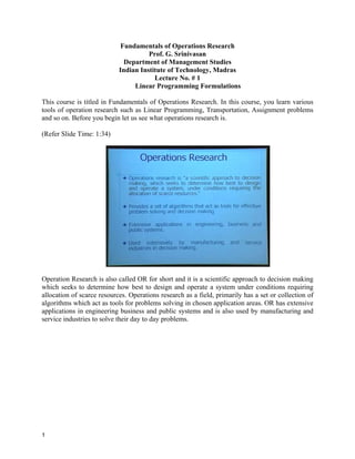
Operation Research is also called OR for short and it is a scientific approach to decision making
which seeks to determine how best to design and operate a system under conditions requiring
allocation of scarce resources. Operations research as a field, primarily has a set or collection of
algorithms which act as tools for problems solving in chosen application areas. OR has extensive
applications in engineering business and public systems and is also used by manufacturing and
service industries to solve their day to day problems.
1

The history of the OR as a field as goes up to the Second World War. In fact this field operations
research started during the Second World War when the British military asked scientists to
analyze military problems. In fact Second World War was perhaps the first time when people
realized that resources were scarce and had to be used effectively and allocated efficiently. The
application of mathematics and scientific methods to military applications was called operations
research to begin with. But today it has a different definition it is also called management
science. A general term Management Science also includes Operation Research. In fact these
two terms are used interchangeably. A set of tools that are used to solve problems is also called
Management Science. Today OR is defined as a scientific approach to decision making that
seeks to determine how best to operate a system under conditions or allocating scarce resources.
In fact the most important thing in operations research is the fact that resources are scarce and
these scarce resources had to be used efficiently.
2

In this course we will primarily handle the above topics. We started with Linear Programming.
We introduced the formulations or problems to formulate it in Linear Programming. We will do
four examples there.
We will also spend lot of time on solving linear programming problems and understand the
various issues associated with the solution. We then get into a specific title called duality and
sensitivity analysis where we explore this linear programming topic further. Then we move on to
two important problems called the Transportation problem and the Assignment problem and
when we do Dynamic Programming and then we also spend some time on Deterministic
Inventory Models. So these will be the topics that will be covered in this course.
3

Linear programming was first conceived by Dantzig, around 1947 at the end of the Second
World War. Very historically, the work of a Russian mathematician first had taken place in 1939
but since it was published in 1959, Dantzig was still credited with starting linear programming.
In fact Dantzig did not use the term linear programming. His first paper was titled ‘Programming
in Linear Structure’. Much later, the term ‘Linear Programming’ was coined by Koopmans. The
Simplex method which is the most popular and powerful tool to solve linear programming
problems, was published by Dantzig in 1949. So this is the brief history of this field called
Linear Programming.
4

(Refer Slide Time: 02)
The first title is called linear programming formulations where we try to introduce to you how to
formulate real life problems as linear programming problems and to understand the various
terminologies that is used in formulating linear programming problems. We begin linear
programming with an example.
So let us consider a small manufacturer making two products called A and B. Two resources are
required which we call as R1 and R2 to make these products. Now each unit of product A
requires one unit of R1 and 3 units of R2.
5

For example we have these two products A and B. Two resources are need R one and R2. A
requires one unit of R1 and three units of R two. B requires one unit of R one and two units of R
two. Manufacturer has 5 units of R one available and 12 units of R two available. The
manufacturer also makes a profit of rupees 6 per unit of A sold and rupees 5 per unit of B of
sold. So this is the problem setting that we are looking at. Now what are the issues that this
manufacturer faces?
(Refer Slide Time: 42)
One, the manufacturer would like to produce in such a way that the profit is maximized. How
does the manufacturer go around formulating his problem?
The first thing is that the manufacturer has to decide on is the number of units of A and B that is
to be produced.
6

It is also reasonable to assume that the manufacturer produces this A and B in such a way to
maximize the profit.
7

So first thing that the manufacturer has to do is to decide or determine how many units of A, and
how many units of B, he or she is going is to produce.
So we first call these as X and Y. So let X be the number of units of A produced and Y be
number of units of B produced. So if the manufacturer produces X units of A and Y units of B
then the money that the person makes or the profit that the person makes, which we call as Z,
will now be 6X + 5Y. Now the manufacturer would ideally like to produce as much of A and as
much of B possible.
8

But what happens is the availability of these resources will now try and restrict the amount of A
and B i.e., X and Y that the manufacturer can produce. So we look at the resource requirement to
produce X of A and Y of B.
So since each unit of A requires one of R1 and each unit of B requires one of R1, the total
amount of resource R1 required is X + (Refer Slide Time 08:42) X + Y. What is available is 5.
This X + Y should not exceed 5 or X + Y is less than or equal to 5. It cannot be more than 5.
Similarly 1 unit of A requires 3 of R2 and 1 unit of B requires two of R2. So the requirement to
produce X units of A and Y units of B is given by 3X + 5Y.
9

This (Refer Slide Time: 9:27) has to be 3X + 2Y and this has to be less than or equal to 12 this
cannot be greater than 12. Also we need to explicitly state that this manufacturer will make X
and Y which are greater than or equal to zero that is the person cannot produce negative
quantities of both X and Y. And you can see this here in this power point slide.
And you can see it here in this power point slide.
10

Also since the person wants to maximize the profit, the profit function Z is to be maximized. So
the person would like to find out X and Y in such a way that the function 6X + 5 Y is maximized
and then X and Y has to satisfy these conditions,
(i) X + Y is less than or equal to 5 and
(ii) 3X + 2 Y less than or equal to 12
And explicitly stating that X and Y has to be greater than or equal to zero which is what is shown
here.
This is called formulating a linear programming problem. What we have done now is we have
converted the descriptive portion that was shown here earlier into a mathematical form and this
mathematical form is called as formulation. Now let us define some amount of terminologies and
we will try to maintain these terminologies consistently in all our formulations. The first thing
11

that we define is called (Refer Slide Time: 10:58 min) decision variables. The two variables that
we solve this problem X and Y are called Decision variables and they represent the output.
Whatever comes out as a solution is going to imply that we make some amount of A and some
amount of B, X amount of A and Y amount of B. The values of X and Y is the output or the
outcome after having solved this problem. So the variables that we want to solve are called
Decision Variables and then we have a function which represents what we are solving this
problem for. And as far as this problem is concerned, we want to solve this problem to maximize
the profit or to get maximum profit and this is the objective with which the manufacturer works.
This function 6X + 5Y represents the profit function which is to be maximized and this is called
the Objective Function. So the second term that is used is called Objective Function which is
precisely the purpose of working on this problem.
12

The third set of things is the Condition. The conditions actually represent the resources that are
available and the resources that have to be used efficiently.
So let these conditions that we have to satisfy namely,
(i) X + Y less than or equal to 5 and
(ii) 3X + 2Y less than or equal to 12 are called constraints because they constrain the
decision variable from taking as larger value as we would ideally like the variable to take.
Because if we simply want to maximize 6X + 5Y without these constraints, then X and Y can
take as higher value as possible. Now these constraints restrict the decision variables form taking
an unlimited or a very high value and so they are important and we have to explicitly state in all
13

linear programming problems (we will define what a linear programming problem is formally)
that these decision variables will have to be greater than or equal to zero.
So the four terms that we have tried to introduce here as you can see some there (Refer Time
Slide: 13:15) are
(i) The decision variables
(ii) The objective function
(iii)Constraints and
(iv)The non-negativity restriction
14

So in a problem in where we define all the four and write it in the mathematical form it is called
formulating a linear programming problem or formulating an operation research problem. (We
will come to the (Refer Slide Time: 13:37) definition a little later).
Now as far as this problem is concerned, X and Y are the Decision variables. The functions 6X +
5Y that is to be maximized is called the Objective function.
X + Y less than or equal to 5 and
3X + 2Y less than or equal to 12 are the Constraints.
X, Y greater than or equal to 0 are the non negativity restriction
15

So the problem formulation has four steps.
 Identifying the decision variables
 Writing the objective function
 Writing the constraints and
 Explicitly stating the non negativity restriction on the variables.
Next, ((Refer Time Slide: 14:17)) in this formulation, we realize that the objective function is a
linear function of the decision variables and all the constraints are linear functions of the decision
variables.
So if you write a formulation such that the objective function is linear and the constraints are
linear then such a formulation is called a Linear Programming Formulation.
16

So the important requirements of a linear programming formulation are that the objective
function is linear, the constraints are linear and we explicitly state that the non negativity
restriction is held.
So these are the three important aspects in a linear programming problem.
If either the objective function or the constraints are Non linear or the case maybe that this does
not exist then it is not a linear programming problem.
17

Now shall look into some more examples to understand the linear programming situation. So this
is the simple formulation where we have looked at two variables, two constraints, and a
maximization objective function.
Now we shall look at more formulations to understand various other aspects of problem
formulation in Linear Programming problems.
Let us look at the second example which is called as Production Planning Problem and the
problem is as follows:
Let us consider a company making a single product demand of 1000, 800, 1200 and 900
respectively for 4 months. Now the company wants to meet the demand for the product in the
next 4 months. The company can use two modes of production. There is something called as
18

Regular Time Production and Overtime Production. Now the regular time capacity is 800/month
and overtime capacity is 200/ month. In order to produce one item in regular time, it costs Rs 20
and to produce overtime it costs Rs 25. The company can also produce more in a particular
month and carry the excess to the next month.
Such a carrying cost is rupees 3. What we call the inventory cost or carrying cost is Rs 3 per unit
per month.
The important condition is that the demand has to be met every month. We cannot afford to have
shortages.
19

Now let’s try to formulate a problem that represents this situation and also try to understand a
few more things about problem formulation as we proceed. Now the first thing we do here is that
we define X1, X2, X3, and X4.
20

Or in general Xj. as quantity produced using regular time production in month j and Yj as
quantity produce using overtime in month j. Now these are our decision variables, Xj and Yj
(quantities that are produced).
Now let us first write the constraints. In fact it is important first to define the decision variables
then to write the objective function & the constraints. Sometimes the constraints can be written
first and then the objective function or sometimes the Objective function & then the constraints
and then explicitly state the non negativity. So in this example we will try the write the
constraints first.
21

Now as far as the first month is concerned, we produce X1 + Y1. We assume that we do not have
any initial inventory or any stock to begin with. So whatever is produced in the first month is X
1+ Y1. We have to meet the first month’s demand which is 1000. So we write X1+ Y1 is greater
than or equal to 1000. We need to produce more than the first month’s demand of 1000. In fact
another alternative is that we can either state X1 + Y1 is greater than or equal to 1000, which
implies that X1 + Y1 is exactly 1000 or more than 1000. If X1+ Y1 is more than 1000 then the
balance is carried to the next month. So we can define another term called I1 which is the
quantity that is carried to the next month.
22

Therefore we can say X1 + Y1 + I1 are equal to 1000. Now for the second month we have
already carried an I1 here (Refer Slide Time: 19:48).
So we start with an I1 and then we produce X2 in regular time. [(Refer Slide Time 19:54)]. X1 +
Y1 = 1000 + I1
The balance is carried i.e., so X1 + Y1-1000 is carried so that is I1. So we begin with I1. We
produce X2 by regular time in the second month and Y2 by overtime in the second month and
that has to be equal to the second month’s demand of 800. Plus, what we carry at the end of the
second month into the third month.
23

So, if this left hand side which is the quantity available at the end of the second month, is more
than the demand which is 800, and if it exceeds 800 then the balance is carried to the third
month.
So here (Refer Slide Time: 20:35), we have this I1 and I2 which are the quantities that are carried
at the end of the month to the next month. Ij is the quantity that is carried at the end of month j to
meet the demand of month j + 1. Similarly for the third one, we begin with I2 to produce X3 +
Y3 which will now be equal to 1200 which we have to meet and if it exceeds 1200, the balance I3
is carried to the fourth month. Now for the fourth month, we begin with I3 to produce X4 + Y4
and that is equal to 900. We are not using an I4 here because the problem stops at the end of the
fourth month and therefore we would adjust these quantities in such a way that we are able to get
exactly 900 which is required to meet the demand of the fourth month. So we do not use an I4
here. Moreover, we also have a situation here wherein all XY Xj Yj and Ij are greater than or
equal to 0.We have to write the objective function. We have not written the objective function as
such.
24

The objective function will be equal to the cost of regular time production. The cost of the
regular time production we have is 20.
25

So 20 into sigma Xj. Sigma Xj represent the total quantities produced in the four months using
the regular time. So 20 into X1 + X2 + X3 + X4 + 25 into the overtime production Yj, if not, you
could say J equal to one to four here (Refer Time Slide : 22:41) and j equal to one to four here. In
addition, whatever quantity that is carried to the next month, we have an additional Rs 3 per unit
per month we have + 3 into sigma Ij, J equal to 1 to 3 and we don’t have I4 in this problem.
Plus, we have Xj, Yj and Ij greater than are equal to 0.
26

Now what is that we want to do? This is the cost function. And this being a cost function, we
would like to minimize this cost function. We like to minimize this cost function.
So now this formulation is complete and this formulation finds out Xj.
Xj, which is the quantity producing using a regular time in month j & Yj which is the quantity
produce using overtime in month j. Constraints are given here and the objective function now
tries to minimize the cost function. So this is the formulation corresponding to the production
planning problem
27

As we go back, as far as the problem is concerned, this has actually 11decision variables (we
have left out the I4).
We need to write some more constraints which have not been written here. The regular time
capacity and the overtime capacity are also given here (Refer Time Slide 24:07). So we need to
write these constraints.
28

These constraints will now be
(i) Xj is less than or equal to 800 for every j
(ii) Yj is less than or equal to two hundred for every j
So we have four constraints here (Refer Slide Time 24:28) we have four more constraints here.
We also have 4 constraints for the 4 months. So we have 12 constraints and we have eleven
variables, 4 variables (X1 to X4) and another four variables (Y1 to Y4) and another three
variables (I1 to I3). So this formulation has a minimization objective which is different from the
maximization objective that we saw in the earlier example. It has twelve constraints and eleven
variables. It also has some equations here (Refer Slide Time 22:52) in the earlier formulation
where we did not have any equation.
29

We also realize that there are constraints which are of the less than or equal to type here in the
earlier formulation as well. We have some equations which are here.
We can do a few more things. From the same formulation we can do a few more things.
30

The first thing is that we can eliminate this I1, I2 and I3 from this (Refer Slide Time 25:39)
which can easily be done.
For example we can eliminate this I1 by saying that X1 + Y1 should be greater than or equal to
1000.
31

Whatever is produced in the first month should be more than or equal to the demand from that
month and if there is an excess it is carried to the second month.
So what could possibly be the excess? The excess will be X1 + Y1 – 1000.
So this becomes X1 + Y1 - 1000 + X2 + Y2 should be greater than or equal to 800. So we
eliminate this I2 as well. Now this quantity is, what is available for the second month this is the
demand for the second month. So if this (Refer Slide Time 26:28) quantity exceeds 800, then the
balance is carried to the third month.
32

So this I2 is nothing but X1+ Y1 + X2 + Y2 -1000-800 will be greater than or equal to 1200 and
we eliminate this three because I2 is nothing but this (Refer Slide Time 26:57) left hand side –
800. So we substitute for I2 here (Refer Slide Time 26:52) to get this and we also eliminate this
I3. We now go back to write what is I3, I3 is nothing but this (Refer Slide Time 27:06) left hand
side minus 1200.
So we eliminate this I3 here and write this as X1 + X2+ X3 + Y1 + Y2+ Y3 –1000–800–1200 =
900 and also we can eliminate these If’s. Now we have the same number of constraints here. We
have few more variables.
33

We have to rewrite the objective function. Also here this objective function has these If’s, so we
have to write this Ij very carefully
So this now becomes + three times (as far as the first month is concerned) X1 + Y1 - 800 + three
times X1 + Y1 – X2 + Y2 – 1800 & (as far as the third month is concerned) X1 + Y1 + X2 + Y2 +
X3 + Y3 – 3000.
34

3000 is the sum of 1800 and 1200.
So this is what is being carried as I3 which comes in. Right now we have not introduced an I4
yet.
35

We have an equation here (Refer Slide Time 28:45).
We can even keep this as greater than or equal to just to be consistent with the other three
constraints and if we choose to do that then what will happen is we have another term that comes
in.
36

You will have a fourth term which is this X1+ Y1 + X2 + Y2 + X3 + Y3 + X4 + Y4 – 3900. We
will continue to have these two constraints Xj less than or equal to 800 and Yj less than or equal
to 200. So you will continue to have these two constraints as well, but the only thing we have
done is we have added another term into the objective function
We have replaced this equation by an inequality just to be consistent with these four so we now
have a second formulation for this problem. We can even have a discussion on this 900. We have
a second formulation for this problem which is the same as what we saw in the first formulation.
37

The only difference is in this formulation, we have fewer variables. We have 12 or even
variables in the earlier one. We now have 8 variables in this formulation. We had equations in
the first one and we now have all inequalities here and we also introduced the greater than or
equal to inequity to this problem which we did not see in the earlier formulations also so this
slightly different formulation but it also represents exactly the same problem that we are trying to
model. Now let us come back to this 900.
38

Now there are two ways of addressing this 900. One is to put an equation here (Refer Slide
Time: 30:45) which will automatically correct the values of X4 and Y4 such that we do not have
anything excess and if we put an equation here.
We can then you can leave out this term.
If you don’t put an equation here and put an inequality instead, it means you are allowing an I4 to
exist and if such an I4 exists then it is carried into the objective function,
39

with the cost of this. Now both are correct.
You can put an equation and leave out this (Refer Slide Time: 31:03) term. You can keep this as
an inequality here and then add this. Both are correct simply because any I4 that is carried from
here comes to increase your cost.
40

So the solution will be such that you will not carry an I4.
And so the I4 will automatically be 0. So in the formulation stage, for the purpose of consistency
you can still keep all these four as inequalities.
41

Then you can write this (Refer Slide Time: 31:36) term. Also, it is just that the objective
function has an additional term that comes into play in this.
This is shown in this slide. The same formulation is shown in this slide. The requirements for the
four months are the four constraints, except that the right hand side is simplified. You can see
that these (Refer Slide Time: 31:55) two terms are taken to the right hand side (as you see the
formulation there) and then you have the same objective function which is shown here (Refer
Slide Term 32:04) including all the four terms,3900 and you will also find that all of them are
inequalities.
42

So this is the second way of formulating this problem. Now when compared to the first, the
question arises as to which one is better? Which one is superior?
There are some very simple guidelines. For the same number of constraints (both these problems
have twelve constraints) you can say that a formulation which has fewer variables is superior.
So this is seen to be the superior one when compared to the earlier. One, both has the same
number of constraints but the number of variables is much less in this.
(Refer Slide Time: 33:06).
43

Also in general, a formulation that has inequalities is better than formulations that have
equations. Most of us are used to solving equations though. Later we see that we convert these
inequalities into equations and so on. But as a very general idea, one may assume that the
formulation which has inequalities is better and preferred over formulations that have equations.
So this is better than the earlier one.
In this formulation, we have learnt a few things like, minimization objective function. The earlier
formulation had a maximization of objective function.
44

In this formulation we learnt to introduce greater than or equal to type inequalities, which we did
not see in the earlier formulation.
Now let us look at a third way to solve the same problem just to show you that the same problem
can have different formulations depending on how you think about the problem.
45

So let us look at the third way to formulate the same problem again. Now we introduced a
slightly different set of decision variables.
Now we are going to introduce Ink as the quantity produced in month I to meet the demand of
month j using production type K. Now we look at four months. So month I can take I equal to
one to four, j can also take j equal to 1 to 4 and K has two types of productions, Regular time and
Overtime. So K takes values 1 or 2. Now with this type of definition of decision variable, let us
try to write the constraints and the objective function corresponding to this problem.
46

As for as the first month is concerned, first month we produced X111 indicates producing in
regular time to meet the first month’s demand using regular time production i.e., producing in the
first month i.e., I equal to one to meet the first month’s demand, j equal to one using regular time
production. It is X111 + X produced in the first month to meet the first month’s demand using
overtime. So these are the only two variables that represent the production to meet the demand of
the first month. So X111 + X112 should be equal to the first month‘s demand which is thousand
1000.
47

Here we are not looking at carrying anything.
You see the way the variables are defined. Whatever quantity that is carried is also defined as a
decision variable.
48

Now we try to meet the second month’s demand. The second month’s demand can be met into
two ways:
(i) by production in the second month
(ii) by production in the first month
In this, we also make an assumption that you cannot meet the first month’s demand by producing
in the later months to be consistent with the earlier assumptions that we made, while you can
actually produce in a month that is early, carry and then meet the demand of subsequent month.
So, the second month’s demand can be met by production in first as well as second. So you have
X121 produced in the first month to meet the demand of the second month by regular time plus
produced in the first month to meet the second month’s demand by overtime plus produced in the
second month to meet the second month’s demand by regular time produced in the second month
to meet the second month’s demand by overtime
So these are the four ways by which you can meet the demands of the second month and these
four should add to the second month’s demand which is 800.
49

Now as far as the third month is concerned, we can meet the third month’s demand by six ways.
(i) Producing in the first month, regular time and overtime
(ii) Producing in second month, regular time and overtime and
(iii)Producing in the third month, regular time and overtime.
So you end up writing X131 produced in the first month to meet the third month’s demand with
regular time + X132 produced in the first month to meet the third month’s demand overtime,
produced in the second month to meet the third month’s demand regular time produced in the
second month, meet the third month’s demand overtime produce in the third month meet third
month’s demand regular time produce in the third month to meet third month’s demand
overtime. This should be exactly equal to 1200 which is the third month’s demand.
50

Now you extend it and write it for the fourth month.
Now this can be done in 8 ways. You can produce in the first month by two ways, second month
by two ways and third month and fourth month two ways. So you have X141 + X142. This
represents producing in the first month to meet the fourth month’s demand by two types. X241 +
X 242 + X 341 + X 342 + X 441 + X 442 are equal to 900. So we have written the four constraints
corresponding to the requirement of the four months. Now we need to look at the constraints on
the capacities.
51

For the first month, the regular time, what we do is, X111, produced in the first month to meet the
demand of the first month by regular time + X121. I produce in the first month to meet to the
demand of the second month, once again by regular time. So when we are looking at the first
month’s regular time production quantity, I will be 1 and k will be 1 but j can be 1, 2, 3, and 4.
So you will have X111 + X121 +X131 + X141. Now these four represent the quantity produced in
the first month, using regular time, to meet the demand of 1, 2, 3 and 4 months. So this should be
less than or equal to the regular time capacity of 800.
Now as far as the second month’s regular time is concerned, you have X produced in second
month to meet the second month’s demand by regular time. So in this case I will be 2 because
you are producing in the second month. k will be 1, since you are using regular time production.
j will be 2,3 or 4 so you will have X221 + X 231 + X 241 should be less than or equal to 800. So as
far as the third month is concerned you will get X331 + X341 because I is equal to 3 represents
producing in the third month j can be 3 or 4. You can produce in the third month to meet the
third month’s requirement or the fourth month’s requirement and k is 1 because you are using
regular time So this should be less than or equal to 800 and as far as the fourth month is
concerned you will have X441 to be less than or equal to 800. You have to write four more for the
overtime production. The only difference being the third subscript will become 2. So the first
month’s overtime will now look like this X112 + X122 + X132 + X142 is less than or equal to 200.
X222 + X232 + X242 is less than or equal to 200. X332 + X342 is less than or equal to 200 and X442
=200. 200 is the capacity that we have. So this (Refer Slide Time 42:38) will also be 200. So
you have these capacity constraints written. Now let us go back and write the objective function.
52

The objective function will look like this. I want to minimize the total cost of regular time,
overtime and the quantity that is carried. So in the first month 20 is the cost of the regular time
production. So I produce X111 + X121 + X131 + X141. Because I can produce by regular time to
meet the demand of all the four. In the second month I produce X221 + X231 + X241 because in the
second month, I can produce only to meet the demands of months 2, 3 and 4. So I have three
terms now. I have X331 + X341 which is the thirds month’s production to meet the demand of
either 3 or 4 and X441. So these are my regular time production quantities. So it is 20 for all these.
Now I have to write a similar term for the overtime production. The only difference is the third
subscript k will become 2 instead of 1.
So I will have + 25 into X112 + X122 + X132 + X142. These four terms represent overtime
production to meet the demands of months 1, 2, 3 and 4. k = implies overtime. Now for the
second month, I will have X222 + X232 + X242.
Once again, as we saw earlier in the second month, you can produce to meet the demand of
months 2, 3 and 4 by overtime. You will have two terms for the third month X332 + X342 and you
will have one term for the fourth month which is X442. Now we also need to write the cost term
corresponding to the quantities that we are carrying.
So what we do is + 3. 3 is the cost that we incur to carry a unit to one month. So all the quantities
that are carried from the first month to second month will come here ((Refer Slide Time 00:46:15
min)) and the one produced in second month carried to third month will come here and produced
in third month carried to the fourth month will come here. For example we will have X121; this is
carried by one month. If j - I = 1, it means it is produced in a particular month and used in the
next month. So it will incur 3. So X121 + X122 are all carried by one month + X231 + X232
produced in the second month to meet the third month produced in the second month to meet the
third month by overtime and X341 + X342. So these are the quantities that are carried one month.
There are quantities that are carried for 2 months. For example, X131 + X132, produced in the first
month to meet only the third months demand so carried to two months with a cost of 6.
Similarly you will have X241 + X242 and there are quantities which are carried to 3 months
because you can produce in the first month and use it in the fourth month. So you will have
another two terms that come in X141 + X142. So this is the objective function. Plus of course, all I
53

or relevant Xijk is greater than or equal to 0. So this is the third type of formulating the same
problem.
You can see that formulation here. You will also observe that this formulation has 20 variables, a
little more than the previous. Ink would allow you 4 into 4 into 2 = 32. But you have only 20
active variables (the other 12 are not active) 12 constraints, you also have some equations. So by
the same discussion that we had had, you realize that this is not a very efficient formulation
compared to the second one.
54

This is because this has more variables.
This also has some equations.
55

Nevertheless this is also a formulation that we can have for the same problem. We have learnt a
few things in the second example which is called the Production Planning example.
The first thing that we learnt is that, there are types of problems which can be formulated as
Minimization problems. The first example was a maximization problem. Second example is the
minimization problem. Objective functions are of two types, Maximization and Minimization.
Both have linear objective functions. So we looked at the second type of objective function,
which is minimization in this case. We also looked at the problem where we introduce the
greater than or equal to constraints.
56

We do not see them here.
You could introduce greater than or equal to constraints when we eliminated the inventory that is
carried.
57

So constraints can be of three types,
(I) less than or equal to type that you see here
(II) Equations that you see here and
(III) Greater than or equal to type.
So we have seen three types of constraints in this. Decision variables of course, are also
included. We have also learnt that a formulation is superior if it has fewer constraints, fewer
variables. It happened that all the three types of formulation had the same number of constraints
so we couldn’t make out something superior based on fewer constraints. But in general a
formulation that has fewer constraints is superior. For the same number of constraints a
formulation that has fewer variables is superior. We also saw that the same problem can be
formulated in more than one way depending on how the person formulating looks at the problem.
Now we did see 3 different types of formulation and all the 3 formulations will give effectively
the same solution if they are correct. Some of them may have more variables. Some of them may
have fewer variables. So we have come across 3 formulations. We also saw the non negativity
restriction that comes in. So in summary in these two examples that we have seen, we have seen
how to formulate a linear programming problem, terminology in terms of Decision variable,
Objective function, Constraints, Non negativity, different types of objectives, different types of
constraints and different types of variables. We later go through two more formulations to
understand some aspects of problem formulation that need to be covered which have not been
covered in these two.
58

Lec1

Recommended

Recommended

More Related Content

What's hot

What's hot (19)

Viewers also liked

Viewers also liked (14)

Similar to Lec1

Similar to Lec1 (20)

Recently uploaded

Recently uploaded (20)

Lec1