1. Polygons as lights: algebraic approximation of polygonal area lights.
Alexander Petryaev.
In CG, the realism of illumination from area lights is due to their naturalness - because most of the
natural light sources we observe in everyday life are in fact area lights. Yet in real-time computer
graphics, area lights are represented mostly in some sort of pre-calculated form because of their
computational expensiveness.
The method presented below allows us to easily introduce illumination from arbitrary planar
polygonal area lights in real-time shading.
Approximation of diffuse illumination.
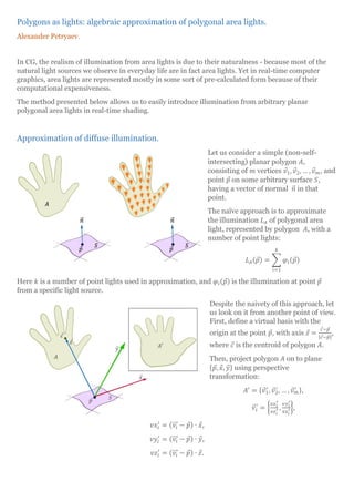
Let us consider a simple (non-self-
intersecting) planar polygon 𝐴,
consisting of 𝑚 vertices 𝑣⃗1, 𝑣⃗2, … , 𝑣⃗ 𝑚, and
point 𝑝⃗ on some arbitrary surface 𝑆,
having a vector of normal 𝑛⃗⃗ in that
point.
The naïve approach is to approximate
the illumination 𝐿 𝐴 of polygonal area
light, represented by polygon 𝐴, with a
number of point lights:
𝐿 𝐴(𝑝⃗) = ∑ 𝜑𝑖(𝑝⃗)
𝑘
𝑖=1
Here 𝑘 is a number of point lights used in approximation, and 𝜑𝑖(𝑝⃗) is the illumination at point 𝑝⃗
from a specific light source.
Despite the naivety of this approach, let
us look on it from another point of view.
First, define a virtual basis with the
origin at the point 𝑝⃗, with axis 𝑧⃗ =
𝑐⃗−𝑝⃗
|𝑐⃗−𝑝⃗|
,
where 𝑐⃗ is the centroid of polygon 𝐴.
Then, project polygon 𝐴 on to plane
{𝑝⃗, 𝑥⃗, 𝑦⃗} using perspective
transformation:
𝐴′
= {𝑣⃗1
′
, 𝑣⃗2
′
, … , 𝑣⃗ 𝑚
′ },
𝑣⃗𝑖
′
= {
𝑣𝑥 𝑖
′
𝑣𝑧𝑖
′ ,
𝑣𝑦𝑖
′
𝑣𝑧𝑖
′},
𝑣𝑥𝑖
′
= (𝑣𝑖⃗⃗⃗⃗ − 𝑝⃗) ∙ 𝑥⃗,
𝑣𝑦𝑖
′
= (𝑣𝑖⃗⃗⃗⃗ − 𝑝⃗) ∙ 𝑦⃗,
𝑣𝑧𝑖
′
= (𝑣𝑖⃗⃗⃗⃗ − 𝑝⃗) ∙ 𝑧⃗.

2. Now, consider applying the similar approximation approach to the transformed polygon 𝐴′
. Let's try
to approximate the illumination from this polygon by a number of light sources, arranged on a
regular square grid with step 𝜎. In addition, assume that all light sources will contribute to the
illumination equally, and that this contribution is proportional to the area of the grid cell:
𝜑′(𝑝⃗) = 𝐼𝐴 ∙ 𝜎2
,
𝐿 𝐴′(𝑝⃗) = ∑ 𝜑′(𝑝⃗)
𝑘
𝑖=1
= 𝐼𝐴 ∙ ∑ 𝜎2
𝑘
𝑖=1
Here 𝐼𝐴 is coefficient of proportionality, semantically close to the intensity of the approximated area
light source.
Obviously, with the value of 𝑘 → ∞ and the value of 𝜎 → 0 the sum above will converge to the area of
polygon 𝐴′
, which is trivially calculated:
𝐿 𝐴′(𝑝⃗) = 𝐼𝐴 ∙ 𝑎𝑟𝑒𝑎(𝐴′)
𝑎𝑟𝑒𝑎(𝐴′) =
1
2
(𝑣𝑥1
′
∙ 𝑣𝑦2
′
− 𝑣𝑥2
′
∙ 𝑣𝑦1
′
+ ⋯ + 𝑣𝑥 𝑚−1
′
∙ 𝑣𝑦 𝑚
′
− 𝑣𝑥 𝑚
′
∙ 𝑣𝑦 𝑚−1
′ )
To summarize this part: the
approximated value of diffuse
illumination from the planar
polygonal area light at the given
point is proportional to the area
of the polygon in the
perspective projection
originated at the given point.

3. Local occlusion of area light.
Since the polygon 𝐴 is planar, the normal of its plane may be easily calculated:
𝑛⃗⃗ 𝐴 =
(𝑣⃗2 − 𝑣⃗1) × (𝑣⃗3 − 𝑣⃗1)
|(𝑣⃗2 − 𝑣⃗1) × (𝑣⃗3 − 𝑣⃗1)|
The equation above supposes that vertices are in a clockwise order and do not lie on the same line.
With normal 𝑛⃗⃗ 𝐴 of polygon 𝐴 and position of its centroid 𝑐⃗ (though any of polygon’s vertices may be
used instead of the centroid) it is possible to rule out the illumination of points behind the polygon:
𝑛⃗⃗ 𝐴 ∙ (𝑐⃗ − 𝑝⃗) > 0 → 𝑝𝑜𝑖𝑛𝑡 𝑝⃗ 𝑙𝑎𝑦𝑠 𝑏𝑒ℎ𝑖𝑛𝑑 𝑡ℎ𝑒 𝑝𝑜𝑙𝑦𝑔𝑜𝑛 𝐴
At the same time, the illumination of points
ahead of the polygon still depends on surface
𝑆, because the surface itself may occlude -
partially or fully - the polygon 𝐴.
Of course, knowing only the vector of normal 𝑛⃗⃗
of the surface 𝑆 at the point 𝑝⃗ it is impossible
to determine global occlusion of the polygon by
the surface. Yet there is enough data to
calculate local occlusion, caused by the surface
in the immediate vicinity of point 𝑝⃗.
Any point 𝑎⃗ of polygon 𝐴 is locally occluded by
surface 𝑆, if the distance from this point to the
plane, defined by point 𝑝⃗ and normal 𝑛⃗⃗, is
negative:
𝑎⃗ ∙ 𝑛⃗⃗ − 𝑝⃗ ∙ 𝑛⃗⃗ < 0 → 𝑝𝑜𝑖𝑛𝑡 𝑎⃗ 𝑖𝑠 𝑙𝑜𝑐𝑎𝑙𝑙𝑦 𝑜𝑐𝑐𝑙𝑢𝑑𝑒𝑑 𝑏𝑦 𝑠𝑢𝑟𝑓𝑎𝑐𝑒 𝑆
Though algorithmically such splitting of the
polygon is trivial, it is still challenging in
shaders because it involves allocation and
manipulation of data structures in imperative
form, which is unnatural for shading
languages, restricted by register-based
memory management.
Suppose 𝐶𝐴 is a circumscribed circle of
polygon 𝐴 with circumcenter at point 𝑜⃗ 𝐴 and
with radius 𝑟𝐶 𝐴
= |𝑜⃗ 𝐴 − 𝑣⃗1|. Then it is possible
to roughly approximate the value of local
occlusion as following:
𝑙𝑜𝑐(𝑝⃗, 𝑛⃗⃗, 𝑜⃗ 𝐴, 𝑟𝐶 𝐴
) =
{
𝑑 ≤ −𝑟𝐶 𝐴
→ 0
𝑑 ≥ 𝑟𝐶 𝐴
→ 1
−𝑟𝐶 𝐴
< 𝑑 < 𝑟𝐶 𝐴
→
𝑑 + 𝑟𝐶 𝐴
2 ∙ 𝑟𝐶 𝐴
𝑑 = 𝑜⃗ 𝐴 ∙ 𝑛⃗⃗ − 𝑝⃗ ∙ 𝑛⃗⃗

4. Here value of 𝑙𝑜𝑐(𝑝⃗, 𝑛⃗⃗, 𝑜⃗ 𝐴, 𝑟𝐶 𝐴
) = 0 means that polygon 𝐴 is fully occluded, value of 𝑙𝑜𝑐(𝑝⃗, 𝑛⃗⃗, 𝑜⃗ 𝐴, 𝑟𝐶 𝐴
) = 1
means that polygon 𝐴 is fully visible and value of 0 < 𝑙𝑜𝑐(𝑝⃗, 𝑛⃗⃗, 𝑜⃗ 𝐴, 𝑟𝐶 𝐴
) < 1 means that polygon 𝐴 is
partially occluded. Note that the approximation above is not good for polygons with an actual area
that greatly differs from the area of corresponding circumscribed circles.
Optimal projection basis.
Some of the readers have probably already found a flaw in the described approximation method. Yes,
it is about the choosing of the basis for projection. Choosing the centroid of the polygon as a control
point for the basis is fine while the
polygon is far enough from the
illuminated point. At a close distance,
some of the transformed vertices may
appear behind the projection plane,
which makes further calculations invalid.
Slightly better results give choosing the control point using weighting coefficients:
𝑐⃗(𝑝⃗) =
1
∑
1
|𝑣⃗𝑖 − 𝑝⃗|
𝑚
𝑖=1
∙ ∑ 𝑣⃗𝑖 ∙
1
|𝑣⃗𝑖 − 𝑝⃗|
𝑚
𝑖=1
Still the optimal basis for projection must preserve all transformed vertices ahead of the projection
plane. There is a problem similar to this one in analytical geometry. It is finding the right irregular
pyramid by given directions of its edges. In the right pyramid an apex lies directly above the centroid
of the base polygon and therefore the vector of height is collinear to the normal of the base plane of
the pyramid.
For the apex take the origin and for directions of edges - subtraction of point 𝑝⃗ from each of polygon
vertices 𝑣⃗𝑖 then the problem is finding of scalars 𝑡𝑖 such that:
𝐶⃗(𝑡1, 𝑡2, … , 𝑡 𝑚)
|𝐶⃗(𝑡1, 𝑡2, … , 𝑡 𝑚)|
∙ 𝑁⃗⃗⃗(𝑡1, 𝑡2, … , 𝑡 𝑚) ≡ −1
𝐶⃗(𝑡1, 𝑡2, … , 𝑡 𝑚) = 𝑐𝑒𝑛𝑡𝑟𝑜𝑖𝑑 𝑜𝑓 𝑝𝑜𝑙𝑦𝑔𝑜𝑛 {(𝑣⃗1 − 𝑝⃗) ∙ 𝑡1, (𝑣⃗2 − 𝑝⃗) ∙ 𝑡2, … , (𝑣⃗ 𝑚 − 𝑝⃗) ∙ 𝑡 𝑚}
𝑁⃗⃗⃗(𝑡1, 𝑡2, … , 𝑡 𝑚) = 𝑛𝑜𝑟𝑚𝑎𝑙 𝑜𝑓 𝑝𝑜𝑙𝑦𝑔𝑜𝑛 {(𝑣⃗1 − 𝑝⃗) ∙ 𝑡1, (𝑣⃗2 − 𝑝⃗) ∙ 𝑡2, … , (𝑣⃗ 𝑚 − 𝑝⃗) ∙ 𝑡 𝑚}
For the case of simplex (polygon 𝐴 is triangle), the problem is less abstract:
1
3
(𝑒⃗1 + 𝑒⃗2 ∙ 𝑡2 + 𝑒⃗3 ∙ 𝑡3)
|
1
3
(𝑒⃗1 + 𝑒⃗2 ∙ 𝑡2 + 𝑒⃗3 ∙ 𝑡3)|
∙
(𝑒⃗2 ∙ 𝑡2 − 𝑒⃗1) × (𝑒⃗3 ∙ 𝑡3 − 𝑒⃗2 ∙ 𝑡2)
|(𝑒⃗2 ∙ 𝑡2 − 𝑒⃗1) × (𝑒⃗3 ∙ 𝑡3 − 𝑒⃗2 ∙ 𝑡2)|
≡ −1
𝑒⃗𝑖 = (𝑣⃗𝑖 − 𝑝⃗)
𝑡1 = 1

5. As you can see, even the case of simplex is rather tough. For the time being, I adopt biased projection
basis as the solution for the area lights located too close to the illuminated surface:
𝑧⃗ =
𝑐⃗ − 𝑝⃗
|𝑐⃗ − 𝑝⃗|
𝑧⃗ 𝑏𝑖𝑎𝑠𝑒𝑑 =
𝑐⃗ − 𝑝⃗ − 𝑧⃗ ∙ 𝑏𝑖𝑎𝑠
|𝑐⃗ − 𝑝⃗ − 𝑧⃗ ∙ 𝑏𝑖𝑎𝑠|
Unfortunately, biased projection affects the shape of the light spot. It is especially noticeable in the
case of elongated polygons.
Results.
The visual results are quite promising.

6. Special bonus: local occlusion works perfectly with normal map.
To measure
performance I have
filled the whole screen
(1440x740) with
fragments illuminated
by a different number
of quadrilateral area
lights. I have used
GeForce GTX 960 as
the hardware to run
the performance tests.
Though the nature of
oscillations at the
beginning of graph is
behind my
comprehension.

7. Future research.
I foresee there are many ways to improve the presented technique:
 Find a better solution for optimal projection basis.
 Develop a proper algorithm for the calculation of a precise local occlusion.
 Find a way to approximate specular illumination.
 Research the applicability of technique for global illumination, including inter-reflections,
global occluders and shadows.
 Research substitution of constant coefficient of proportionality 𝐼𝐴 by functions.
External resources.
Link to GitHub repository (Unity3D project): https://github.com/bad3p/PAL