Dimitri Solomatine - Hydroinformatics

AGUA 2009

Hydroinformatics
and some of its roles in the view
of climate variability

Dr. Dimitri P. Solomatine
Professor of Hydroinformatics

1

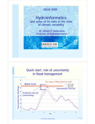
Quick start: role of uncertainty
in flood management
80

So, issue a flood alarm or not?..
70
Alarm level O est i m e
U
ne at
pper bound
Forecasted river discharge

Low bound
er
60
Deterministic forecast
50
Prediction interval
Di schar ge

40 (uncertainty)
30

20

10

0
1 11 21 31 41 51
Ti me

2
D.P. Solomatine. Hydroinformatics.

Climate is changing…

http://www.globalwarmingart.com/wiki/File:Holocene_Temperature_Variations_Rev_png 3

Global warming

4

Variability in annual temperatures locally
Source: www.john-daly.com, based on data from NASA Goddard Institute (GISS), USA,
and Climatic Research Unit (CRU) of the University of East Anglia, Norwich, UK

5

Climate is changing…

There are many factors leading to
changes in the rate of climate change
Whatever the main reason is, the climate variations prompt for
developing the water management strategies
that take climate uncertainties into account

the need for
More observation systems
Better predictive modelling tools
Analytical methods to handle uncertainty
Changes in design and adaptive management practices
Changes in educational programmes at all levels
These issues are the current focus of Hydroinformatics 6

Encapsulation of knowledge
related to water
Tacit (implicit) knowledge embedded within a person
Words, texts, images
printed
stored in electronic media
Mathematical models
formulas, algorithms
algorithms encapsulated in computer programs
(software)
Integrated systems encapsulating all of above -
Hydroinformatics systems

7

Hydroinformatics

modelling, information
and communication technology,
computer sciences

applied to
problems of aquatic
environment 1991

with the purpose of
proper management
2008
8

Flow of information in a Hydroinformatics system
Data Models Knowledge Decisions

Earth observation, Numerical Weather Data modelling, Access to Decision
monitoring Prediction Models integration with modelling support
hydrologic and results
hydraulic models

Map of flood probability

9

Where is data coming from?

10

∂Q ∂ ⎛ Q 2 ⎞ ∂h
+ ⎜ ⎜ A ⎟ + gA ∂x − gAS o + gAS f = 0
⎟
∂t ∂x ⎝ ⎠

Modelling
is the heart of Hydroinformatics

11

Modelling

Model is …
a simplified description of reality
an encapsulation of knowledge about a particular physical or
social process in electronic form

Goals of modelling are:
understand the studied system or domain (the past)
predict the future
use the results of modelling for making decisions (change
the future)

12

Modelling is at heart of Hydroinformatics

Hydroinformatics deals with the technologies ensuring the
whole information cycle, and integrates
data,
models,
people

13

Main modelling paradigms

Physically-based model (process, simulation, numerical) is
based on the understanding of the underlying processes

Data-driven model is based on the recorded values of
variables characterising the system. They need less
knowledge about the physical behaviour

Agent-based model consists of dynamically interacting
relatively simple rule-based computational codes (agents)

14

Applications of models

River/urban flood forecasting and management
Reservoir operations
Sediment transport and morphology
Ecology and water quality
Storm surges and coastal flooding
Dredging and reclamation
Urban sewers and drainage
Water distribution networks
etc.

15

Example: a physically-based model of open
channel flow: Saint Venant equations

The 1D continuity and momentum equations for open
channel flow are also referred as Saint Venant equation
Form a pair of non-linear hyperbolic partial differential equations
in Q (flow) and h (depth)
∂A ∂Q
+ = qL Continuity equation
∂t ∂x
∂Q ∂ ⎛ Q 2 ⎞ ∂h
+ ⎜ ⎜ A ⎟ + gA ∂x − gAS o + gAS f = 0
⎟
Momentum equation
∂t ∂x ⎝ ⎠
x=distance, t=time, A=cross-section, S0=bottom slope, Sf=energy grade line slope, B=width
Analytically can not be solved
Numerically can be solved using
finite differences (explicit, implicit schemes),
finite elements
16

Why 2D/3D modelling?
Often 1D model is not enough

Horizontal velocity fields Vertical velocity fields

17

Some examples of using modelling
in water-related issues

18

Warragamba Dam, Australia

Warragamba Dam - 65 km west of
Sydney in the Burragorang Valley
provides the major water supply for
Sydney
Warragamba River flows through a
300-600 m wide gorge, about 100 m
deep before opening out into a large
valley. This allows a relatively short
and high dam to impound a vast
quantity of water.
A dam break of the Warragamba
Dam would be a major disaster.
SOBEK (Delft Hydraulics) software
was used for simulation 19

Warragamba Dam, Australia
Simulation of the dam break with SOBEK by Deltares

The animation shows the simulation results. They may be
used for disaster management, evacuation planning, flood
damage assessment, urban planning

20

Models are indispensable in dealing with floods

21

Example: Hydroinformatics systems for flood
warning – MIKE FloodWatch

MIKE Flood Watch (Danish Hydraulic Institute), a decision
support system for real-time flood forecasting:
advanced time series data base
MIKE 11, for hydrodynamic modeling
MIKE 11 FF, real-time forecasting system,
ArcView, Geographical Information System (GIS)

22

Hydroinformatics systems for flood warning:
MIKE FloodWatch

23

Ecosystem Integrated Model:
a Case Study for Sonso Lake, Colombia

Problem: 70% of the surface area of this shallow lake
is covered by an invasive macrophite Water Hyacinth
Causes:
Nutrients pollution from agricultural use of land
Lack of sustainable management of the lake
Methodology:
Ecological modelling of Water Hyacinth
Its integration with hydrodynamic model
Analysis of Alternatives to Manage the Water Hyacinth
Infestation

24

Ecosystem Integrated Model:
a Case Study for Sonso Lake, Colombia
Ref: MSc study by Carlos Velez (Colombia), UNESCO-IHE & Delft Hydraulics

Solar
WATER SURFACE Radiation
2 3 5
6 16
Sobek Rural Sobek Rural 1 Water Volume 15
1D2D DELWAQ 5 13
Norg Porg
7 9 10 Water
Velocity 14
Hydro Water 4 NH4 Hyacinth
dynamic Water Depth 11
Quality PO4 12
Flow 6 NO3
8 9
Ecosystem SEDIMENT
Organic Matter Settled

PROCESSES
Water Hyacinth 1. Input / Output 5. Input / Output 9. Resuspension 13. Photosynthesis
Model (coded 2. Rainfall 6. Input / Output 10. Hydrolysis 14. Respiration
using SOBEK 3. Evapotranspiration 7. Sedimentation 11. Oxidation 15. Mortality
RURAL Open 4. Advection/Dispersion 8. Resuspension 12. Uptake/Growth 16. Losses
25
Process Library) D.P. Solomatine. Hydroinformatics.

Hydrodynamic Model 1D River and Nutrients Model (Phosphate PO4)
2D Lake (Water Level)

Processes included:
Growth and Mortality
Respiration/Photosynthesis
Transportation by flow and wind
Uptake/release of Nutrients from
the water
Mechanical, Biological and
Chemical Control Options

Water Hyacinth Integrated Model
(Plant Density)
26

Beyond “classical” modelling:
current developments in Hydroinformatics

Machine learning in data-driven modelling

Multi-objective optimisation

Information theory

Predicting models’ uncertainty

Integration
27

Data-Driven Modelling

Uses (numerical) data (time series) describing some
physical process
Establishes functions that link variables
outputs = F (inputs)
Valuable when physical processes are unknown
Also useful as emulators of complex physically-based
models (surrogate models)

Actual (observed)
Modelled output Y
Input data X (real)
system
Learning is aimed
at minimizing this
Machine difference
learning
(data-driven)
model Predicted output Y’
28

Example of a data-driven model
Linear regression model
Y = a0 + a1 X
observed data characterises the
Y
input-output relationship actual
output (e.g., flow)
X Y value

model parameters are found by
optimization model
predicts new
the model then predicts output output value

for the new input without actual
knowledge of what drives Y
new input X
value (e.g. rainfall)

Which model is “better”:
green, red or blue?
29

Data-driven rainfall-runoff models:
Case study Sieve (Italy)

mountaneous
catchment in Southern
Europe
area of 822 sq. km

30

SIEVE: visualization of data
FLOW1: effective rainfall and discharge data Discharge [m3/s]
Eff.rainfall [mm]
800 0
2
700
4
600
Effective rainfall [mm] 6
500
8
400 10
Discharge [m3/s]
12
300
14
200
16
100
18
0 20
0 500 1000 1500 2000 2500
Time [hrs]

variables for building a decision tree model were selected on the basis of
cross-correlation analysis and average mutual information:
inputs: rainfalls REt, REt-1, REt-2, REt-3, flows Qt, Qt-1
outputs: flows Qt+1 or Qt+3 Solomatine. Hydroinformatics.
D.P.
31

Using data-driven methods in
rainfall-runoff modelling
Qtup
Available data:
rainfalls Rt
runoffs (flows) Qt
Inputs: lagged rainfalls Rt Rt-1 … Rt-L Rt Qt
Output to predict: Qt+T

Model: Qt+T = F (Rt Rt-1 … Rt-L … Qt Qt-1 Qt-A … Qtup Qt-1up …)
(past rainfall) (autocorrelation) (routing)

Questions:
how to find the appropriate lags?
how to build non-linear regression function F ?
Linear regression, neural network, support vector machine etc.

32

Artificial neural network: a universal function
approximator (=non-linear regression model)

weights weights
x1 a ij b jk y1 ⎛ N hid ⎞
x2
u 1x
y2
yk = F ⎜ bok +
⎜
⎝
∑ b jk u j ⎟
⎟
⎠
i =1
x3 y3
k=1,..., N out

xn us ym
Inputs Hidden layer Outputs
F(v)
⎛ N inp ⎞ 1
uj = F ⎜ aoj +
⎜ ∑ aij xi ⎟
⎟
⎝ i =1 ⎠
0 v
j=1,..., N hid
Non-linear sigmoid function: F(v) = 1/ (1 + e-v)
There are (Ninp+1)Nhid + (Nhid+1)Nout parameters (weights) to be identified by
optimisation process (training)

33

Neural network tool interface

34

SIEVE: Predicting Q(t+3) three hours ahead
(ANN learned the relationship btw rainfall and flow)

Prediction of Qt+3 : Verification performance
ANN verification
350
RMSE=11.353
NRMSE=0.234 300 Observed
Modelled (ANN)
COE=0.9452 250 Modelled (MT)
Q [ m 3 /s ]
200
MT verification
RMSE=12.548 150
NRMSE=0.258 100
COE=0.9331
50

0
0 20 40 60 80 100 120 140 160 180
t [hrs]

35

Use of machine learning (data-driven) models
in water resources

Hydrological modelling
Water demand forecasting
Prediction of ocean surges
Models of wind-wave interaction
Sedimentation modelling

Meta-models (emulating, fast models) of water systems –
to replace complex physically-based models

36

MULTI-OBJECTIVE OPTIMIZATION

Finding variables’ values that bring the value of the
“objective function” to a minimum
In water resources many problems require solving an
optimization problem

37

Many optimization problems in water
resources are multi-objective

there are several objectives that are to be optimized
often they are in conflict, i.e. minimizing one does not
mean minimizing another one
a solution (the set of decision variables) is always a
compromise
Examples:
multi-purpose reservoir operation
electricity generation vs. irrigation vs. navigability
models calibration (error minimization)
models good "on average" vs. good for particular hydrologic
conditions (floods)
pipe networks optimization (design and rehabilitation)
costs vs. reduction of flood damage

38

Model-based optimization of urban drainage
network

MOUSE modelling system (DHI
Water and Environment)
1D model of free-surface flow
is used

39

Urban drainage system rehabilitation:
use of multi-objective optimization
rehabilitation: changing pipes, creating additional storages
optimization by multi-objective genetic algorithm:
find a compromise btw. min. cost and min. damage due to flooding

Compromise
Flood Damage

optimal solutions
Wastewater System Pipe
Network Model (MOUSE)
Data Processor Data Processor
Optimization Procedure Costs
(GLOBE, NSGA-II)
40

INFORMATION THEORY
Shannon entropy provides a mathematical framework to evaluate
the amount of information contained in a data series

H = −∑ p log2 p
Average mutual information (AMI) is measure of information
available from one set of data having knowledge of another set
of data
AMI can be used to investigate dependencies and lag effects in
time series data
⎡ PXY ( xi , y j ) ⎤
AMI= ∑ PXY ( xi , y j ) log 2 ⎢ ⎥
i, j ⎢ PX ( xi ) P ( y j ) ⎥
⎣ Y ⎦
41

Information theory and optimization
for sensors locations for contaminant detection
in water distribution systems
Three criteria considered:
Concentration
Volume of contaminated water delivered
Time of detection

PhD research of Mr. Leonardo Alfonso, UNESCO-IHE.
L. Alfonso , A. Jonoski , D.P. Solomatine. Multi-objective optimisation of operational responses
for contaminant flushing in water distribution networks. ASCE J. Water Res. Plan.Manag., 2009. 42

Multi-objective optimization of sensors
locations to detect contamination
Location of 5 sensors
Scenario: 2 sources of pollution
Time of Detection
40 50
Contaminated Volume
Contaminant concentration
501
Tank A 80 140
60
30

90 150

170
502
100 Tank B
70
160

130

500 20 110
120
Source
Locations found using different method
43

Average mutual information in optimizing the
structure of a Neural Network model

Rainfall-runoff forecasting model: Rt Qt
Qt+T = F (Rt Rt-1 … Rt-L … Qt Qt-1 Qt-A)
(past rainfall) (autocorrelation)

Finding optimal lags between Qt+T and rainfall Rt
1.0 0.30

0.8 0.25

0.20
Corr. Coef.

0.6
AMI

0.15
0.4
0.10
0.2 0.05

0.0 0.00
0 5 10 15 20
Time lags (hours)
Cross-correlation Autocorrelation AMI

44

UNCERTAINTY

Uncertainties associated with climate change are very high
Different IPCC scenarios lead to very different results of
water models
Any study exploring the impacts of CC needs powerful
tools for analysing and predicting uncertainty

45

Uncertainty in flood management:
evacuate?
80

70 O est i m e
ne at
Upper bound
Low bound
er
60

50
Di schar ge

40

30

20

10

0
1 11 21 31 41 51
Ti me

46

Point forecasts vs. Uncertainty bounds

4000

3500

3000
Discharge(m3/s)

2500

2000

1500

1000

500

0
900 920 940 960 980 1000 1020
Time(days)
47

Sources of uncertainty in modelling
y = M(x, s, θ) + εs + εθ + εx + εy
Inputs Model parameters Calibration data

p
X(t) Q(t)

Model
48

Monte Carlo simulation of parametric uncertainty
y = M(x, s, θ) + εs + εθ + εx + εy

49

80

Uncertainty analysis: issues
70 O est i m e
ne at
Upper bound
Low bound
er
60

50
Di schar ge

40

30

20

10

0
1 11 21 31 41 51
Ti me

Most methods are aimed at analysing average model uncertainty, but
not predicting it for the new inputs
Most uncertainty analysis studies focus on the parametric uncertainty
only. More has to be done to analyse and predict:
Input data uncertainty
Residual uncertainty (uncertainty associated with the deficiencies
of the “optimal” model)
Model uncertainty is estimated. What next?:
Should we combine in an ensemble several “good” models,
instead of using one calibrated model?
How can we predict model uncertainty for the future situations?
How to communicate uncertainty to decision makers?

50

UNEEC: Novel uncertainty prediction method
D.P. Solomatine, D.L. Shrestha. A novel method to estimate model uncertainty using machine
learning techniques. Water Resources Res., 45, W00B11, doi:10.1029/ 2008WR006839, 2009.

A calibrated model M of a water system is considered
M is run for the past hydrometeorological events
It is assumed that the errors of model M characterize the
“residual” uncertainty in different situations (events)
This data is used to train the machine learning model U
that predicts the error (uncertainty) of model M, which is
specific for a particular hydrometeorological event

UNEEC-M: parametric and input uncertainty is added as
well

51

UNEEC: fuzzy clustering and ANN in
encapsulating the model uncertainty

Error limits past records
Error distribution in cluster Error (or prediction (examples in the
intervals)
∑ μi
N
∑ μi
i =1
space of inputs)
N
(1 − α / 2) ∑ μi
i =1

Flow Qt-1
N
α / 2 ∑ μi
i =1

Train regression (ANN)
Prediction interval models:
PIL = fL (X)
PIU = fU (X)

Rainfall Rt-2 New record. The trained f
L and f U models will

estimate the prediction
interval
52

Estimated prediction bounds: verification
(Bagmati river basin, Nepal)
Rainfall-Discharge plot

6000 0
50
5000
100

Precip itation [mm]
Runoff [Cumec]
4000
150
3000 200
250
2000
300
1000
350
0 400

Jan-88
M ay-88
Sep-88
Feb-89
Jun-89
Oct-89
M ar-90
Jul-90
Nov-90
Apr-91
Aug-91
Jan-92
M ay-92
Sep-92
Feb-93
Jun-93
Oct-93
M ar-94
Jul-94
Dec-94
Apr-95
Aug-95
Time [days]

Runoff [Cumec] Precipitation [mm]

4000
90% prediction limits

Observed flow (m /s)
Observed flow
3000

3
SF – Snow
RF – Rain
EA – Evapotranspiration
SP – Snow cover
SF
RF IN – Infiltration 2000
EA R – Recharge
SM – Soil moisture
CFLUX – Capillary transport
SP UZ – Storage in upper reservoir
IN
PERC – Percolation 1000
SM
LZ – Storage in lower reservoir
R CFLUX Qo – Fast runoff component
Q0 Q1 – Slow runoff component
UZ Q – Total runoff
0
PERC Q1 Q=Q0+Q1 750 775 800 825 850
LZ Transform
Time(day) 53
function

Hydroinformatics is about
INTEGRATION
of data, models and people

54

Integration of atmospheric, hydro- and
environmental models, data systems

HBV

55

Integration of models, communications
and people

Internet – models on demand, distributed DSS
Mobile telephony – a channel for hazards warnings and
advice systems

Ref: MSc by L. Alfonso (Colombia), UNESCO-IHE
56

Integration of Hydroinformatics systems and
decision making

Multi-criteria, multi-stakeholder 80

scenario analysis 70 O est i m e
ne at
Upper bound

Communication of model
Low bound
er
60

uncertainty to managers
50

Di schar ge
40

30

20

10

0
1 11 21 31 41 51
Ti me

Map of flood probability

57

Education:
Hydroinformatics at UNESCO-IHE,
Delft, The Netherlands

58

Postgraduate Education, Training
and Capacity Building
in Water, Environment and Infrastructure

59

UNESCO-IHE: 14,000 Alumni

UNESCO-IHE Alumni Community

0 - 50 51-150 151-300 301-500 501-850 851-1200
60

Hydroinformatics Masters programme
Fundamentals, hydraulic, hydrologic and environmental processes
Information systems, GIS, communications, Internet
• ArcGIS • Matlab • JAVA
• Access Tools • Delphi • UltraDev

Physically-based
Physically- • SOBEK • MIKE 11

simulation modelling
• RIBASIM
• Delft 3D
• HEC-RAS
HEC-
• MIKE 21
with applications to:
and tools
• SWAT • MIKE SHE - River basin management
• EPANET • RIBASIM
• MOUSE • WEST++ - Flood management
Data-driven modelling
Data- • Aquarius • MODFLOW
- Urban systems
and computational • NeuroSolutions - Coastal systems
• NeuralMachine
intelligence tools • AFUZ - Groundwater and
• WEKA
catchment hydrology
Systems analysis, • LINGO
- Environmental systems
decision support, • GLOBE
• BSCW (options)
optimization • AquaVoice

Integration of technologies, project management

Elective advanced topics
61

Hydroinformatics Study Modules

Introduction to Water science and Engineering
Applied Hydraulics and hydrology
Geo-information systems
Computational Hydraulics and Information Management
Modelling theory and applications
Computational Intelligence and Control Systems
River Basin Modelling
Fieldtrip to Florida, USA
Selective modelling subjects (2 modules each):
Flood risk management
Urban water systems modelling
Environmental systems modelling
Hydroinformatics for Decision Support
Groupwork
Research proposal drafting and Special Topics
MSc research

62

Examples of MSc topics

Hydroinformatics for real time water quality management and
operation of distribution networks, case study Villavicencio, Colombia
Water distribution modelling with intermittent supply: sensitivity
analysis and performance evaluation for Bani-Suhila City, Palestine
Urban Flood Warning System with wireless technology, case study of
Dhaka City, Bangladesh
Flood modelling and forecasting for Awash river basin in Ethiopia
Harmful Algal Bloom prediction, study of Western Xiamen Bay, China
Application of Neural Networks to rainfall-runoff modelling in the
upper reach of the Huai river basin, China
Heihe River Basin Water Resources Decision Support System
Decision Support System for Irrigation Management in Vietnam
1D-2D Coupling Urban Flooding Model using radar data in Bangkok
Using chaos theory to predict ocean surge
63

A new programme is planned:
International Masters in Hydroinformatics
UNESCO-IHE – UniValle-Cinara
Hidroinformática
modelación y sistemas de información para la gestión del agua
Programa Internacional de Maestría en Ciencia

jointly delivered by
UNESCO-IHE Institute for Water Education,
Delft, The Netherlands
and
Universidad del Valle (UNIVALLE, Cinara),
Cali, Colombia
and leading to the degree
of Master of Science in Water Science and Engineering, specialisation in
Hydroinformatics,
accredited by the Dutch Ministry of Education

Planned to start in September 2010
Fliers are available Hydroinformatics.
D.P. Solomatine.
64

Programme structure
Taught part
Block 1: Location: UNIVALLE, Cali ECTS
Fundamental subjects for 15
hydroinformatics
Period: September-January

Block 2: Location UNESCO-IHE
Hydroinformatics theory and
Period: Mid-January – end-August: 9
applications
modules of the existing UNESCO-IHE ECTS
WSE-HI programme (modules 4-12) 45

Thesis part
Block 3: Location: Any of the core partners (in
MSc thesis proposal the beginning UNESCO-IHE)
preparation + special topics
Period: Begin-September – Mid-
October ECTS
10

Block 4: Location: Any of the core or the
MSc Thesis research associated partners (at least the last
month at UNESCO-IHE)
ECTS
Period: Mid-October – mid-April. 36
Public MSc defence and graduation –
end of April
65

What Hydroinformatics alumni say...

the course has opened the new horizons
in my professional life

66

Conclusion

Hydroinformatics is a unifying approach to water
modelling and management
Specialists in hydroinformatics play an integrating role
linking various specialists and decision makers
Access to information by widening groups of stakeholders
leads to democratisation of water services
One of the roles of Hydroinformatics is developing
analytical methods to deal with climatic variability in
modelling and management practice
Focus should be on education and training

67

…more data is needed…
68

Dimitri Solomatine - Hydroinformatics

Recommended

Recommended

More Related Content

Viewers also liked

Viewers also liked (10)

Similar to Dimitri Solomatine - Hydroinformatics

Similar to Dimitri Solomatine - Hydroinformatics (20)

Dimitri Solomatine - Hydroinformatics