1. Lectures on Lévy Processes and Stochastic
Calculus (Koc University)
Lecture 2: Lévy Processes
David Applebaum
School of Mathematics and Statistics, University of Sheffield, UK
6th December 2011
Dave Applebaum (Sheffield UK) Lecture 2 December 2011 1 / 56
2. Definition: Lévy Process
Let X = (X (t), t ≥ 0) be a stochastic process defined on a probability
space (Ω, F, P).
We say that it has independent increments if for each n ∈ N and each
0 ≤ t1 < t2 < · · · < tn+1 < ∞, the random variables
(X (tj+1 ) − X (tj ), 1 ≤ j ≤ n) are independent
and it has stationary increments if each
d
X (tj+1 ) − X (tj ) = X (tj+1 − tj ) − X (0).
Dave Applebaum (Sheffield UK) Lecture 2 December 2011 2 / 56
3. Definition: Lévy Process
Let X = (X (t), t ≥ 0) be a stochastic process defined on a probability
space (Ω, F, P).
We say that it has independent increments if for each n ∈ N and each
0 ≤ t1 < t2 < · · · < tn+1 < ∞, the random variables
(X (tj+1 ) − X (tj ), 1 ≤ j ≤ n) are independent
and it has stationary increments if each
d
X (tj+1 ) − X (tj ) = X (tj+1 − tj ) − X (0).
Dave Applebaum (Sheffield UK) Lecture 2 December 2011 2 / 56
4. Definition: Lévy Process
Let X = (X (t), t ≥ 0) be a stochastic process defined on a probability
space (Ω, F, P).
We say that it has independent increments if for each n ∈ N and each
0 ≤ t1 < t2 < · · · < tn+1 < ∞, the random variables
(X (tj+1 ) − X (tj ), 1 ≤ j ≤ n) are independent
and it has stationary increments if each
d
X (tj+1 ) − X (tj ) = X (tj+1 − tj ) − X (0).
Dave Applebaum (Sheffield UK) Lecture 2 December 2011 2 / 56
5. We say that X is a Lévy process if
(L1) Each X (0) = 0 (a.s),
(L2) X has independent and stationary increments,
(L3) X is stochastically continuous i.e. for all a > 0 and for all s ≥ 0,
lim P(|X (t) − X (s)| > a) = 0.
t→s
Note that in the presence of (L1) and (L2), (L3) is equivalent to the
condition
lim P(|X (t)| > a) = 0.
t↓0
Dave Applebaum (Sheffield UK) Lecture 2 December 2011 3 / 56
6. We say that X is a Lévy process if
(L1) Each X (0) = 0 (a.s),
(L2) X has independent and stationary increments,
(L3) X is stochastically continuous i.e. for all a > 0 and for all s ≥ 0,
lim P(|X (t) − X (s)| > a) = 0.
t→s
Note that in the presence of (L1) and (L2), (L3) is equivalent to the
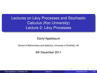
condition
lim P(|X (t)| > a) = 0.
t↓0
Dave Applebaum (Sheffield UK) Lecture 2 December 2011 3 / 56
7. We say that X is a Lévy process if
(L1) Each X (0) = 0 (a.s),
(L2) X has independent and stationary increments,
(L3) X is stochastically continuous i.e. for all a > 0 and for all s ≥ 0,
lim P(|X (t) − X (s)| > a) = 0.
t→s
Note that in the presence of (L1) and (L2), (L3) is equivalent to the
condition
lim P(|X (t)| > a) = 0.
t↓0
Dave Applebaum (Sheffield UK) Lecture 2 December 2011 3 / 56
8. We say that X is a Lévy process if
(L1) Each X (0) = 0 (a.s),
(L2) X has independent and stationary increments,
(L3) X is stochastically continuous i.e. for all a > 0 and for all s ≥ 0,
lim P(|X (t) − X (s)| > a) = 0.
t→s
Note that in the presence of (L1) and (L2), (L3) is equivalent to the
condition
lim P(|X (t)| > a) = 0.
t↓0
Dave Applebaum (Sheffield UK) Lecture 2 December 2011 3 / 56
9. The sample paths of a process are the maps t → X (t)(ω) from R+ to
Rd , for each ω ∈ Ω.
We are now going to explore the relationship between Lévy processes
and infinite divisibility.
Theorem
If X is a Lévy process, then X (t) is infinitely divisible for each t ≥ 0.
Dave Applebaum (Sheffield UK) Lecture 2 December 2011 4 / 56
10. The sample paths of a process are the maps t → X (t)(ω) from R+ to
Rd , for each ω ∈ Ω.
We are now going to explore the relationship between Lévy processes
and infinite divisibility.
Theorem
If X is a Lévy process, then X (t) is infinitely divisible for each t ≥ 0.
Dave Applebaum (Sheffield UK) Lecture 2 December 2011 4 / 56
11. The sample paths of a process are the maps t → X (t)(ω) from R+ to
Rd , for each ω ∈ Ω.
We are now going to explore the relationship between Lévy processes
and infinite divisibility.
Theorem
If X is a Lévy process, then X (t) is infinitely divisible for each t ≥ 0.
Dave Applebaum (Sheffield UK) Lecture 2 December 2011 4 / 56
12. Proof. For each n ∈ N, we can write
(n) (n)
X (t) = Y1 (t) + · · · + Yn (t)
where each Yk (t) = X ( kt ) − X ( (k −1)t ).
(n)
n n
(n)
The Yk (t)’s are i.i.d. by (L2). 2
From Lecture 1 we can write φX (t) (u) = eη(t,u) for each t ≥ 0, u ∈ Rd ,
where each η(t, ·) is a Lévy symbol.
Dave Applebaum (Sheffield UK) Lecture 2 December 2011 5 / 56
13. Proof. For each n ∈ N, we can write
(n) (n)
X (t) = Y1 (t) + · · · + Yn (t)
where each Yk (t) = X ( kt ) − X ( (k −1)t ).
(n)
n n
(n)
The Yk (t)’s are i.i.d. by (L2). 2
From Lecture 1 we can write φX (t) (u) = eη(t,u) for each t ≥ 0, u ∈ Rd ,
where each η(t, ·) is a Lévy symbol.
Dave Applebaum (Sheffield UK) Lecture 2 December 2011 5 / 56
14. Proof. For each n ∈ N, we can write
(n) (n)
X (t) = Y1 (t) + · · · + Yn (t)
where each Yk (t) = X ( kt ) − X ( (k −1)t ).
(n)
n n
(n)
The Yk (t)’s are i.i.d. by (L2). 2
From Lecture 1 we can write φX (t) (u) = eη(t,u) for each t ≥ 0, u ∈ Rd ,
where each η(t, ·) is a Lévy symbol.
Dave Applebaum (Sheffield UK) Lecture 2 December 2011 5 / 56
15. Theorem
If X is a Lévy process, then
φX (t) (u) = etη(u) ,
for each u ∈ Rd , t ≥ 0, where η is the Lévy symbol of X (1).
Proof. Suppose that X is a Lévy process and for each u ∈ Rd , t ≥ 0,
define φu (t) = φX (t) (u)
then by (L2) we have for all s ≥ 0,
φu (t + s) = E(ei(u,X (t+s)) )
= E(ei(u,X (t+s)−X (s)) ei(u,X (s)) )
= E(ei(u,X (t+s)−X (s)) )E(ei(u,X (s)) )
= φu (t)φu (s) . . . (i)
Dave Applebaum (Sheffield UK) Lecture 2 December 2011 6 / 56
16. Theorem
If X is a Lévy process, then
φX (t) (u) = etη(u) ,
for each u ∈ Rd , t ≥ 0, where η is the Lévy symbol of X (1).
Proof. Suppose that X is a Lévy process and for each u ∈ Rd , t ≥ 0,
define φu (t) = φX (t) (u)
then by (L2) we have for all s ≥ 0,
φu (t + s) = E(ei(u,X (t+s)) )
= E(ei(u,X (t+s)−X (s)) ei(u,X (s)) )
= E(ei(u,X (t+s)−X (s)) )E(ei(u,X (s)) )
= φu (t)φu (s) . . . (i)
Dave Applebaum (Sheffield UK) Lecture 2 December 2011 6 / 56
17. Theorem
If X is a Lévy process, then
φX (t) (u) = etη(u) ,
for each u ∈ Rd , t ≥ 0, where η is the Lévy symbol of X (1).
Proof. Suppose that X is a Lévy process and for each u ∈ Rd , t ≥ 0,
define φu (t) = φX (t) (u)
then by (L2) we have for all s ≥ 0,
φu (t + s) = E(ei(u,X (t+s)) )
= E(ei(u,X (t+s)−X (s)) ei(u,X (s)) )
= E(ei(u,X (t+s)−X (s)) )E(ei(u,X (s)) )
= φu (t)φu (s) . . . (i)
Dave Applebaum (Sheffield UK) Lecture 2 December 2011 6 / 56
18. Theorem
If X is a Lévy process, then
φX (t) (u) = etη(u) ,
for each u ∈ Rd , t ≥ 0, where η is the Lévy symbol of X (1).
Proof. Suppose that X is a Lévy process and for each u ∈ Rd , t ≥ 0,
define φu (t) = φX (t) (u)
then by (L2) we have for all s ≥ 0,
φu (t + s) = E(ei(u,X (t+s)) )
= E(ei(u,X (t+s)−X (s)) ei(u,X (s)) )
= E(ei(u,X (t+s)−X (s)) )E(ei(u,X (s)) )
= φu (t)φu (s) . . . (i)
Dave Applebaum (Sheffield UK) Lecture 2 December 2011 6 / 56
19. Theorem
If X is a Lévy process, then
φX (t) (u) = etη(u) ,
for each u ∈ Rd , t ≥ 0, where η is the Lévy symbol of X (1).
Proof. Suppose that X is a Lévy process and for each u ∈ Rd , t ≥ 0,
define φu (t) = φX (t) (u)
then by (L2) we have for all s ≥ 0,
φu (t + s) = E(ei(u,X (t+s)) )
= E(ei(u,X (t+s)−X (s)) ei(u,X (s)) )
= E(ei(u,X (t+s)−X (s)) )E(ei(u,X (s)) )
= φu (t)φu (s) . . . (i)
Dave Applebaum (Sheffield UK) Lecture 2 December 2011 6 / 56
20. Theorem
If X is a Lévy process, then
φX (t) (u) = etη(u) ,
for each u ∈ Rd , t ≥ 0, where η is the Lévy symbol of X (1).
Proof. Suppose that X is a Lévy process and for each u ∈ Rd , t ≥ 0,
define φu (t) = φX (t) (u)
then by (L2) we have for all s ≥ 0,
φu (t + s) = E(ei(u,X (t+s)) )
= E(ei(u,X (t+s)−X (s)) ei(u,X (s)) )
= E(ei(u,X (t+s)−X (s)) )E(ei(u,X (s)) )
= φu (t)φu (s) . . . (i)
Dave Applebaum (Sheffield UK) Lecture 2 December 2011 6 / 56
21. x
Now φu (0) = 1 . . . (ii) by (L1), and the map t → φu (t) is continuous.
However the unique continuous solution to (i) and (ii) is given by
φu (t) = etα(u) , where α : Rd → C. Now by Theorem 1, X (1) is infinitely
divisible, hence α is a Lévy symbol and the result follows.
2
Dave Applebaum (Sheffield UK) Lecture 2 December 2011 7 / 56
22. x
Now φu (0) = 1 . . . (ii) by (L1), and the map t → φu (t) is continuous.
However the unique continuous solution to (i) and (ii) is given by
φu (t) = etα(u) , where α : Rd → C. Now by Theorem 1, X (1) is infinitely
divisible, hence α is a Lévy symbol and the result follows.
2
Dave Applebaum (Sheffield UK) Lecture 2 December 2011 7 / 56
23. x
Now φu (0) = 1 . . . (ii) by (L1), and the map t → φu (t) is continuous.
However the unique continuous solution to (i) and (ii) is given by
φu (t) = etα(u) , where α : Rd → C. Now by Theorem 1, X (1) is infinitely
divisible, hence α is a Lévy symbol and the result follows.
2
Dave Applebaum (Sheffield UK) Lecture 2 December 2011 7 / 56
24. x
Now φu (0) = 1 . . . (ii) by (L1), and the map t → φu (t) is continuous.
However the unique continuous solution to (i) and (ii) is given by
φu (t) = etα(u) , where α : Rd → C. Now by Theorem 1, X (1) is infinitely
divisible, hence α is a Lévy symbol and the result follows.
2
Dave Applebaum (Sheffield UK) Lecture 2 December 2011 7 / 56
25. x
Now φu (0) = 1 . . . (ii) by (L1), and the map t → φu (t) is continuous.
However the unique continuous solution to (i) and (ii) is given by
φu (t) = etα(u) , where α : Rd → C. Now by Theorem 1, X (1) is infinitely
divisible, hence α is a Lévy symbol and the result follows.
2
Dave Applebaum (Sheffield UK) Lecture 2 December 2011 7 / 56
26. We now have the Lévy-Khinchine formula for a Lévy
process X = (X (t), t ≥ 0):-
1
E(ei(u,X (t)) ) = exp{ t i(b, u) − (u, Au)
2
+ (ei(u,y ) − 1 − i(u, y )1B (y ))ν(dy )
ˆ },(2.1)
Rd −{0}
for each t ≥ 0, u ∈ Rd , where (b, A, ν) are the characteristics of X (1).
We will define the Lévy symbol and the characteristics of a Lévy
process X to be those of the random variable X (1). We will sometimes
write the former as ηX when we want to emphasise that it belongs to
the process X .
Dave Applebaum (Sheffield UK) Lecture 2 December 2011 8 / 56
27. We now have the Lévy-Khinchine formula for a Lévy
process X = (X (t), t ≥ 0):-
1
E(ei(u,X (t)) ) = exp{ t i(b, u) − (u, Au)
2
+ (ei(u,y ) − 1 − i(u, y )1B (y ))ν(dy )
ˆ },(2.1)
Rd −{0}
for each t ≥ 0, u ∈ Rd , where (b, A, ν) are the characteristics of X (1).
We will define the Lévy symbol and the characteristics of a Lévy
process X to be those of the random variable X (1). We will sometimes
write the former as ηX when we want to emphasise that it belongs to
the process X .
Dave Applebaum (Sheffield UK) Lecture 2 December 2011 8 / 56
28. We now have the Lévy-Khinchine formula for a Lévy
process X = (X (t), t ≥ 0):-
1
E(ei(u,X (t)) ) = exp{ t i(b, u) − (u, Au)
2
+ (ei(u,y ) − 1 − i(u, y )1B (y ))ν(dy )
ˆ },(2.1)
Rd −{0}
for each t ≥ 0, u ∈ Rd , where (b, A, ν) are the characteristics of X (1).
We will define the Lévy symbol and the characteristics of a Lévy
process X to be those of the random variable X (1). We will sometimes
write the former as ηX when we want to emphasise that it belongs to
the process X .
Dave Applebaum (Sheffield UK) Lecture 2 December 2011 8 / 56
29. Let pt be the law of X (t), for each t ≥ 0. By (L2), we have for all
s, t ≥ 0 that:
pt+s = pt ∗ ps .
w
By (L3), we have pt → δ0 as t → 0, i.e. limt→0 f (x)pt (dx) = f (0).
(pt , t ≥ 0) is a weakly continuous convolution semigroup of probability
measures on Rd .
Conversely, given any such semigroup, we can always construct a
Lévy process on path space via Kolmogorov’s construction.
Dave Applebaum (Sheffield UK) Lecture 2 December 2011 9 / 56
30. Let pt be the law of X (t), for each t ≥ 0. By (L2), we have for all
s, t ≥ 0 that:
pt+s = pt ∗ ps .
w
By (L3), we have pt → δ0 as t → 0, i.e. limt→0 f (x)pt (dx) = f (0).
(pt , t ≥ 0) is a weakly continuous convolution semigroup of probability
measures on Rd .
Conversely, given any such semigroup, we can always construct a
Lévy process on path space via Kolmogorov’s construction.
Dave Applebaum (Sheffield UK) Lecture 2 December 2011 9 / 56
31. Let pt be the law of X (t), for each t ≥ 0. By (L2), we have for all
s, t ≥ 0 that:
pt+s = pt ∗ ps .
w
By (L3), we have pt → δ0 as t → 0, i.e. limt→0 f (x)pt (dx) = f (0).
(pt , t ≥ 0) is a weakly continuous convolution semigroup of probability
measures on Rd .
Conversely, given any such semigroup, we can always construct a
Lévy process on path space via Kolmogorov’s construction.
Dave Applebaum (Sheffield UK) Lecture 2 December 2011 9 / 56
32. Let pt be the law of X (t), for each t ≥ 0. By (L2), we have for all
s, t ≥ 0 that:
pt+s = pt ∗ ps .
w
By (L3), we have pt → δ0 as t → 0, i.e. limt→0 f (x)pt (dx) = f (0).
(pt , t ≥ 0) is a weakly continuous convolution semigroup of probability
measures on Rd .
Conversely, given any such semigroup, we can always construct a
Lévy process on path space via Kolmogorov’s construction.
Dave Applebaum (Sheffield UK) Lecture 2 December 2011 9 / 56
33. Let pt be the law of X (t), for each t ≥ 0. By (L2), we have for all
s, t ≥ 0 that:
pt+s = pt ∗ ps .
w
By (L3), we have pt → δ0 as t → 0, i.e. limt→0 f (x)pt (dx) = f (0).
(pt , t ≥ 0) is a weakly continuous convolution semigroup of probability
measures on Rd .
Conversely, given any such semigroup, we can always construct a
Lévy process on path space via Kolmogorov’s construction.
Dave Applebaum (Sheffield UK) Lecture 2 December 2011 9 / 56
34. Informally, we have the following asymptotic relationship between the
law of a Lévy process and its Lévy measure:
pt
ν = lim .
t↓0 t
More precisely
1
lim f (x)pt (dx) = f (x)ν(dx), (2.2)
t↓0 t Rd Rd
for bounded, continuous functions f which vanish in some
neighborhood of the origin.
Dave Applebaum (Sheffield UK) Lecture 2 December 2011 10 / 56
35. Informally, we have the following asymptotic relationship between the
law of a Lévy process and its Lévy measure:
pt
ν = lim .
t↓0 t
More precisely
1
lim f (x)pt (dx) = f (x)ν(dx), (2.2)
t↓0 t Rd Rd
for bounded, continuous functions f which vanish in some
neighborhood of the origin.
Dave Applebaum (Sheffield UK) Lecture 2 December 2011 10 / 56
36. Informally, we have the following asymptotic relationship between the
law of a Lévy process and its Lévy measure:
pt
ν = lim .
t↓0 t
More precisely
1
lim f (x)pt (dx) = f (x)ν(dx), (2.2)
t↓0 t Rd Rd
for bounded, continuous functions f which vanish in some
neighborhood of the origin.
Dave Applebaum (Sheffield UK) Lecture 2 December 2011 10 / 56
37. Examples of Lévy Processes
Example 1, Brownian Motion and Gaussian Processes
A (standard) Brownian motion in Rd is a Lévy process
B = (B(t), t ≥ 0) for which
(B1) B(t) ∼ N(0, tI) for each t ≥ 0,
(B2) B has continuous sample paths.
It follows immediately from (B1) that if B is a standard Brownian
motion, then its characteristic function is given by
1
φB(t) (u) = exp{− t|u|2 },
2
for each u ∈ Rd , t ≥ 0.
Dave Applebaum (Sheffield UK) Lecture 2 December 2011 11 / 56
38. Examples of Lévy Processes
Example 1, Brownian Motion and Gaussian Processes
A (standard) Brownian motion in Rd is a Lévy process
B = (B(t), t ≥ 0) for which
(B1) B(t) ∼ N(0, tI) for each t ≥ 0,
(B2) B has continuous sample paths.
It follows immediately from (B1) that if B is a standard Brownian
motion, then its characteristic function is given by
1
φB(t) (u) = exp{− t|u|2 },
2
for each u ∈ Rd , t ≥ 0.
Dave Applebaum (Sheffield UK) Lecture 2 December 2011 11 / 56
39. Examples of Lévy Processes
Example 1, Brownian Motion and Gaussian Processes
A (standard) Brownian motion in Rd is a Lévy process
B = (B(t), t ≥ 0) for which
(B1) B(t) ∼ N(0, tI) for each t ≥ 0,
(B2) B has continuous sample paths.
It follows immediately from (B1) that if B is a standard Brownian
motion, then its characteristic function is given by
1
φB(t) (u) = exp{− t|u|2 },
2
for each u ∈ Rd , t ≥ 0.
Dave Applebaum (Sheffield UK) Lecture 2 December 2011 11 / 56
40. Examples of Lévy Processes
Example 1, Brownian Motion and Gaussian Processes
A (standard) Brownian motion in Rd is a Lévy process
B = (B(t), t ≥ 0) for which
(B1) B(t) ∼ N(0, tI) for each t ≥ 0,
(B2) B has continuous sample paths.
It follows immediately from (B1) that if B is a standard Brownian
motion, then its characteristic function is given by
1
φB(t) (u) = exp{− t|u|2 },
2
for each u ∈ Rd , t ≥ 0.
Dave Applebaum (Sheffield UK) Lecture 2 December 2011 11 / 56
41. We introduce the marginal processes Bi = (Bi (t), t ≥ 0) where each
Bi (t) is the ith component of B(t), then it is not difficult to verify that the
Bi ’s are mutually independent Brownian motions in R. We will call
these one-dimensional Brownian motions in the sequel.
Brownian motion has been the most intensively studied Lévy process.
In the early years of the twentieth century, it was introduced as a
model for the physical phenomenon of Brownian motion by Einstein
and Smoluchowski and as a description of the dynamical evolution of
stock prices by Bachelier.
Dave Applebaum (Sheffield UK) Lecture 2 December 2011 12 / 56
42. We introduce the marginal processes Bi = (Bi (t), t ≥ 0) where each
Bi (t) is the ith component of B(t), then it is not difficult to verify that the
Bi ’s are mutually independent Brownian motions in R. We will call
these one-dimensional Brownian motions in the sequel.
Brownian motion has been the most intensively studied Lévy process.
In the early years of the twentieth century, it was introduced as a
model for the physical phenomenon of Brownian motion by Einstein
and Smoluchowski and as a description of the dynamical evolution of
stock prices by Bachelier.
Dave Applebaum (Sheffield UK) Lecture 2 December 2011 12 / 56
43. We introduce the marginal processes Bi = (Bi (t), t ≥ 0) where each
Bi (t) is the ith component of B(t), then it is not difficult to verify that the
Bi ’s are mutually independent Brownian motions in R. We will call
these one-dimensional Brownian motions in the sequel.
Brownian motion has been the most intensively studied Lévy process.
In the early years of the twentieth century, it was introduced as a
model for the physical phenomenon of Brownian motion by Einstein
and Smoluchowski and as a description of the dynamical evolution of
stock prices by Bachelier.
Dave Applebaum (Sheffield UK) Lecture 2 December 2011 12 / 56
44. We introduce the marginal processes Bi = (Bi (t), t ≥ 0) where each
Bi (t) is the ith component of B(t), then it is not difficult to verify that the
Bi ’s are mutually independent Brownian motions in R. We will call
these one-dimensional Brownian motions in the sequel.
Brownian motion has been the most intensively studied Lévy process.
In the early years of the twentieth century, it was introduced as a
model for the physical phenomenon of Brownian motion by Einstein
and Smoluchowski and as a description of the dynamical evolution of
stock prices by Bachelier.
Dave Applebaum (Sheffield UK) Lecture 2 December 2011 12 / 56
45. We introduce the marginal processes Bi = (Bi (t), t ≥ 0) where each
Bi (t) is the ith component of B(t), then it is not difficult to verify that the
Bi ’s are mutually independent Brownian motions in R. We will call
these one-dimensional Brownian motions in the sequel.
Brownian motion has been the most intensively studied Lévy process.
In the early years of the twentieth century, it was introduced as a
model for the physical phenomenon of Brownian motion by Einstein
and Smoluchowski and as a description of the dynamical evolution of
stock prices by Bachelier.
Dave Applebaum (Sheffield UK) Lecture 2 December 2011 12 / 56
46. We introduce the marginal processes Bi = (Bi (t), t ≥ 0) where each
Bi (t) is the ith component of B(t), then it is not difficult to verify that the
Bi ’s are mutually independent Brownian motions in R. We will call
these one-dimensional Brownian motions in the sequel.
Brownian motion has been the most intensively studied Lévy process.
In the early years of the twentieth century, it was introduced as a
model for the physical phenomenon of Brownian motion by Einstein
and Smoluchowski and as a description of the dynamical evolution of
stock prices by Bachelier.
Dave Applebaum (Sheffield UK) Lecture 2 December 2011 12 / 56
47. The theory was placed on a rigorous mathematical basis by Norbert
Wiener in the 1920’s.
We could try to use the Kolmogorov existence theorem to construct
one-dimensional Brownian motion from the following prescription on
cylinder sets of the form
ItH,...,tn = {ω ∈ Ω; ω(t1 ) ∈ [a1 , b1 ], . . . , ω(tn ) ∈ [an , bn ]} where
1
H = [a1 , b1 ] × · · · [an , bn ] and we have taken Ω to be the set of all
mappings from R+ to R:
P(ItH,...,tn )
1
2
1 1 x1 (x2 − x1 )2
= n exp − + + ··
H (2π) 2 t1 (t2 − t1 ) . . . (tn − tn−1 ) 2 t1 t2 − t1
(xn − xn−1 )2
+ dx1 · · · dxn .
tn − tn−1
However there there is then no guarantee that the paths are
continuous.
Dave Applebaum (Sheffield UK) Lecture 2 December 2011 13 / 56
48. The theory was placed on a rigorous mathematical basis by Norbert
Wiener in the 1920’s.
We could try to use the Kolmogorov existence theorem to construct
one-dimensional Brownian motion from the following prescription on
cylinder sets of the form
ItH,...,tn = {ω ∈ Ω; ω(t1 ) ∈ [a1 , b1 ], . . . , ω(tn ) ∈ [an , bn ]} where
1
H = [a1 , b1 ] × · · · [an , bn ] and we have taken Ω to be the set of all
mappings from R+ to R:
P(ItH,...,tn )
1
2
1 1 x1 (x2 − x1 )2
= n exp − + + ··
H (2π) 2 t1 (t2 − t1 ) . . . (tn − tn−1 ) 2 t1 t2 − t1
(xn − xn−1 )2
+ dx1 · · · dxn .
tn − tn−1
However there there is then no guarantee that the paths are
continuous.
Dave Applebaum (Sheffield UK) Lecture 2 December 2011 13 / 56
49. The theory was placed on a rigorous mathematical basis by Norbert
Wiener in the 1920’s.
We could try to use the Kolmogorov existence theorem to construct
one-dimensional Brownian motion from the following prescription on
cylinder sets of the form
ItH,...,tn = {ω ∈ Ω; ω(t1 ) ∈ [a1 , b1 ], . . . , ω(tn ) ∈ [an , bn ]} where
1
H = [a1 , b1 ] × · · · [an , bn ] and we have taken Ω to be the set of all
mappings from R+ to R:
P(ItH,...,tn )
1
2
1 1 x1 (x2 − x1 )2
= n exp − + + ··
H (2π) 2 t1 (t2 − t1 ) . . . (tn − tn−1 ) 2 t1 t2 − t1
(xn − xn−1 )2
+ dx1 · · · dxn .
tn − tn−1
However there there is then no guarantee that the paths are
continuous.
Dave Applebaum (Sheffield UK) Lecture 2 December 2011 13 / 56
50. The theory was placed on a rigorous mathematical basis by Norbert
Wiener in the 1920’s.
We could try to use the Kolmogorov existence theorem to construct
one-dimensional Brownian motion from the following prescription on
cylinder sets of the form
ItH,...,tn = {ω ∈ Ω; ω(t1 ) ∈ [a1 , b1 ], . . . , ω(tn ) ∈ [an , bn ]} where
1
H = [a1 , b1 ] × · · · [an , bn ] and we have taken Ω to be the set of all
mappings from R+ to R:
P(ItH,...,tn )
1
2
1 1 x1 (x2 − x1 )2
= n exp − + + ··
H (2π) 2 t1 (t2 − t1 ) . . . (tn − tn−1 ) 2 t1 t2 − t1
(xn − xn−1 )2
+ dx1 · · · dxn .
tn − tn−1
However there there is then no guarantee that the paths are
continuous.
Dave Applebaum (Sheffield UK) Lecture 2 December 2011 13 / 56
51. The theory was placed on a rigorous mathematical basis by Norbert
Wiener in the 1920’s.
We could try to use the Kolmogorov existence theorem to construct
one-dimensional Brownian motion from the following prescription on
cylinder sets of the form
ItH,...,tn = {ω ∈ Ω; ω(t1 ) ∈ [a1 , b1 ], . . . , ω(tn ) ∈ [an , bn ]} where
1
H = [a1 , b1 ] × · · · [an , bn ] and we have taken Ω to be the set of all
mappings from R+ to R:
P(ItH,...,tn )
1
2
1 1 x1 (x2 − x1 )2
= n exp − + + ··
H (2π) 2 t1 (t2 − t1 ) . . . (tn − tn−1 ) 2 t1 t2 − t1
(xn − xn−1 )2
+ dx1 · · · dxn .
tn − tn−1
However there there is then no guarantee that the paths are
continuous.
Dave Applebaum (Sheffield UK) Lecture 2 December 2011 13 / 56
52. The literature contains a number of ingenious methods for constructing
Brownian motion. One of the most delightful of these (originally due to
Paley and Wiener) obtains this, in the case d = 1, as a random Fourier
series for 0 ≤ t ≤ 1:
√ ∞
2 sin(πt(n + 1 ))
2
B(t) = 1
ξ(n),
π n+ 2
n=0
for each t ≥ 0, where (ξ(n), n ∈ N) is a sequence of i.i.d. N(0, 1)
random variables.
Dave Applebaum (Sheffield UK) Lecture 2 December 2011 14 / 56
53. The literature contains a number of ingenious methods for constructing
Brownian motion. One of the most delightful of these (originally due to
Paley and Wiener) obtains this, in the case d = 1, as a random Fourier
series for 0 ≤ t ≤ 1:
√ ∞
2 sin(πt(n + 1 ))
2
B(t) = 1
ξ(n),
π n+ 2
n=0
for each t ≥ 0, where (ξ(n), n ∈ N) is a sequence of i.i.d. N(0, 1)
random variables.
Dave Applebaum (Sheffield UK) Lecture 2 December 2011 14 / 56
54. The literature contains a number of ingenious methods for constructing
Brownian motion. One of the most delightful of these (originally due to
Paley and Wiener) obtains this, in the case d = 1, as a random Fourier
series for 0 ≤ t ≤ 1:
√ ∞
2 sin(πt(n + 1 ))
2
B(t) = 1
ξ(n),
π n+ 2
n=0
for each t ≥ 0, where (ξ(n), n ∈ N) is a sequence of i.i.d. N(0, 1)
random variables.
Dave Applebaum (Sheffield UK) Lecture 2 December 2011 14 / 56
55. We list a number of useful properties of Brownian motion in the case
d = 1.
Brownian motion is locally Hölder continuous with exponent α for
every 0 < α < 1 i.e. for every T > 0, ω ∈ Ω there exists
2
K = K (T , ω) such that
|B(t)(ω) − B(s)(ω)| ≤ K |t − s|α ,
for all 0 ≤ s < t ≤ T .
The sample paths t → B(t)(ω) are almost surely nowhere
differentiable.
For any sequence, (tn , n ∈ N) in R+ with tn ↑ ∞,
lim inf B(tn ) = −∞ a.s. lim sup B(tn ) = ∞ a.s.
n→∞ n→∞
The law of the iterated logarithm:-
B(t)
P lim sup 1
=1 = 1.
t↓0 (2t log(log( 1 ))) 2
t
Dave Applebaum (Sheffield UK) Lecture 2 December 2011 15 / 56
56. We list a number of useful properties of Brownian motion in the case
d = 1.
Brownian motion is locally Hölder continuous with exponent α for
every 0 < α < 1 i.e. for every T > 0, ω ∈ Ω there exists
2
K = K (T , ω) such that
|B(t)(ω) − B(s)(ω)| ≤ K |t − s|α ,
for all 0 ≤ s < t ≤ T .
The sample paths t → B(t)(ω) are almost surely nowhere
differentiable.
For any sequence, (tn , n ∈ N) in R+ with tn ↑ ∞,
lim inf B(tn ) = −∞ a.s. lim sup B(tn ) = ∞ a.s.
n→∞ n→∞
The law of the iterated logarithm:-
B(t)
P lim sup 1
=1 = 1.
t↓0 (2t log(log( 1 ))) 2
t
Dave Applebaum (Sheffield UK) Lecture 2 December 2011 15 / 56
57. We list a number of useful properties of Brownian motion in the case
d = 1.
Brownian motion is locally Hölder continuous with exponent α for
every 0 < α < 1 i.e. for every T > 0, ω ∈ Ω there exists
2
K = K (T , ω) such that
|B(t)(ω) − B(s)(ω)| ≤ K |t − s|α ,
for all 0 ≤ s < t ≤ T .
The sample paths t → B(t)(ω) are almost surely nowhere
differentiable.
For any sequence, (tn , n ∈ N) in R+ with tn ↑ ∞,
lim inf B(tn ) = −∞ a.s. lim sup B(tn ) = ∞ a.s.
n→∞ n→∞
The law of the iterated logarithm:-
B(t)
P lim sup 1
=1 = 1.
t↓0 (2t log(log( 1 ))) 2
t
Dave Applebaum (Sheffield UK) Lecture 2 December 2011 15 / 56
58. We list a number of useful properties of Brownian motion in the case
d = 1.
Brownian motion is locally Hölder continuous with exponent α for
every 0 < α < 1 i.e. for every T > 0, ω ∈ Ω there exists
2
K = K (T , ω) such that
|B(t)(ω) − B(s)(ω)| ≤ K |t − s|α ,
for all 0 ≤ s < t ≤ T .
The sample paths t → B(t)(ω) are almost surely nowhere
differentiable.
For any sequence, (tn , n ∈ N) in R+ with tn ↑ ∞,
lim inf B(tn ) = −∞ a.s. lim sup B(tn ) = ∞ a.s.
n→∞ n→∞
The law of the iterated logarithm:-
B(t)
P lim sup 1
=1 = 1.
t↓0 (2t log(log( 1 ))) 2
t
Dave Applebaum (Sheffield UK) Lecture 2 December 2011 15 / 56
59. We list a number of useful properties of Brownian motion in the case
d = 1.
Brownian motion is locally Hölder continuous with exponent α for
every 0 < α < 1 i.e. for every T > 0, ω ∈ Ω there exists
2
K = K (T , ω) such that
|B(t)(ω) − B(s)(ω)| ≤ K |t − s|α ,
for all 0 ≤ s < t ≤ T .
The sample paths t → B(t)(ω) are almost surely nowhere
differentiable.
For any sequence, (tn , n ∈ N) in R+ with tn ↑ ∞,
lim inf B(tn ) = −∞ a.s. lim sup B(tn ) = ∞ a.s.
n→∞ n→∞
The law of the iterated logarithm:-
B(t)
P lim sup 1
=1 = 1.
t↓0 (2t log(log( 1 ))) 2
t
Dave Applebaum (Sheffield UK) Lecture 2 December 2011 15 / 56
60. 1.2
0.8
0.4
0
−0.4
−0.8
−1.2
−1.6
−2.0
0 1 2 3 4 5
Simulation of standard Brownian motion
Dave Applebaum (Sheffield UK) Lecture 2 December 2011 16 / 56
61. Let A be a non-negative symmetric d × d matrix and let σ be a square
root of A so that σ is a d × m matrix for which σσ T = A. Now let b ∈ Rd
and let B be a Brownian motion in R m . We construct a process
C = (C(t), t ≥ 0) in Rd by
C(t) = bt + σB(t), (2.3)
then C is a Lévy process with each C(t) ∼ N(tb, tA). It is not difficult to
verify that C is also a Gaussian process, i.e. all its finite dimensional
distributions are Gaussian. It is sometimes called Brownian motion
with drift. The Lévy symbol of C is
1
ηC (u) = i(b, u) − (u, Au).
2
In fact a Lévy process has continuous sample paths if and only if it is of
the form (2.3).
Dave Applebaum (Sheffield UK) Lecture 2 December 2011 17 / 56
62. Let A be a non-negative symmetric d × d matrix and let σ be a square
root of A so that σ is a d × m matrix for which σσ T = A. Now let b ∈ Rd
and let B be a Brownian motion in R m . We construct a process
C = (C(t), t ≥ 0) in Rd by
C(t) = bt + σB(t), (2.3)
then C is a Lévy process with each C(t) ∼ N(tb, tA). It is not difficult to
verify that C is also a Gaussian process, i.e. all its finite dimensional
distributions are Gaussian. It is sometimes called Brownian motion
with drift. The Lévy symbol of C is
1
ηC (u) = i(b, u) − (u, Au).
2
In fact a Lévy process has continuous sample paths if and only if it is of
the form (2.3).
Dave Applebaum (Sheffield UK) Lecture 2 December 2011 17 / 56
63. Let A be a non-negative symmetric d × d matrix and let σ be a square
root of A so that σ is a d × m matrix for which σσ T = A. Now let b ∈ Rd
and let B be a Brownian motion in R m . We construct a process
C = (C(t), t ≥ 0) in Rd by
C(t) = bt + σB(t), (2.3)
then C is a Lévy process with each C(t) ∼ N(tb, tA). It is not difficult to
verify that C is also a Gaussian process, i.e. all its finite dimensional
distributions are Gaussian. It is sometimes called Brownian motion
with drift. The Lévy symbol of C is
1
ηC (u) = i(b, u) − (u, Au).
2
In fact a Lévy process has continuous sample paths if and only if it is of
the form (2.3).
Dave Applebaum (Sheffield UK) Lecture 2 December 2011 17 / 56
64. Let A be a non-negative symmetric d × d matrix and let σ be a square
root of A so that σ is a d × m matrix for which σσ T = A. Now let b ∈ Rd
and let B be a Brownian motion in R m . We construct a process
C = (C(t), t ≥ 0) in Rd by
C(t) = bt + σB(t), (2.3)
then C is a Lévy process with each C(t) ∼ N(tb, tA). It is not difficult to
verify that C is also a Gaussian process, i.e. all its finite dimensional
distributions are Gaussian. It is sometimes called Brownian motion
with drift. The Lévy symbol of C is
1
ηC (u) = i(b, u) − (u, Au).
2
In fact a Lévy process has continuous sample paths if and only if it is of
the form (2.3).
Dave Applebaum (Sheffield UK) Lecture 2 December 2011 17 / 56
65. Let A be a non-negative symmetric d × d matrix and let σ be a square
root of A so that σ is a d × m matrix for which σσ T = A. Now let b ∈ Rd
and let B be a Brownian motion in R m . We construct a process
C = (C(t), t ≥ 0) in Rd by
C(t) = bt + σB(t), (2.3)
then C is a Lévy process with each C(t) ∼ N(tb, tA). It is not difficult to
verify that C is also a Gaussian process, i.e. all its finite dimensional
distributions are Gaussian. It is sometimes called Brownian motion
with drift. The Lévy symbol of C is
1
ηC (u) = i(b, u) − (u, Au).
2
In fact a Lévy process has continuous sample paths if and only if it is of
the form (2.3).
Dave Applebaum (Sheffield UK) Lecture 2 December 2011 17 / 56
66. Let A be a non-negative symmetric d × d matrix and let σ be a square
root of A so that σ is a d × m matrix for which σσ T = A. Now let b ∈ Rd
and let B be a Brownian motion in R m . We construct a process
C = (C(t), t ≥ 0) in Rd by
C(t) = bt + σB(t), (2.3)
then C is a Lévy process with each C(t) ∼ N(tb, tA). It is not difficult to
verify that C is also a Gaussian process, i.e. all its finite dimensional
distributions are Gaussian. It is sometimes called Brownian motion
with drift. The Lévy symbol of C is
1
ηC (u) = i(b, u) − (u, Au).
2
In fact a Lévy process has continuous sample paths if and only if it is of
the form (2.3).
Dave Applebaum (Sheffield UK) Lecture 2 December 2011 17 / 56
67. Let A be a non-negative symmetric d × d matrix and let σ be a square
root of A so that σ is a d × m matrix for which σσ T = A. Now let b ∈ Rd
and let B be a Brownian motion in R m . We construct a process
C = (C(t), t ≥ 0) in Rd by
C(t) = bt + σB(t), (2.3)
then C is a Lévy process with each C(t) ∼ N(tb, tA). It is not difficult to
verify that C is also a Gaussian process, i.e. all its finite dimensional
distributions are Gaussian. It is sometimes called Brownian motion
with drift. The Lévy symbol of C is
1
ηC (u) = i(b, u) − (u, Au).
2
In fact a Lévy process has continuous sample paths if and only if it is of
the form (2.3).
Dave Applebaum (Sheffield UK) Lecture 2 December 2011 17 / 56
68. Let A be a non-negative symmetric d × d matrix and let σ be a square
root of A so that σ is a d × m matrix for which σσ T = A. Now let b ∈ Rd
and let B be a Brownian motion in R m . We construct a process
C = (C(t), t ≥ 0) in Rd by
C(t) = bt + σB(t), (2.3)
then C is a Lévy process with each C(t) ∼ N(tb, tA). It is not difficult to
verify that C is also a Gaussian process, i.e. all its finite dimensional
distributions are Gaussian. It is sometimes called Brownian motion
with drift. The Lévy symbol of C is
1
ηC (u) = i(b, u) − (u, Au).
2
In fact a Lévy process has continuous sample paths if and only if it is of
the form (2.3).
Dave Applebaum (Sheffield UK) Lecture 2 December 2011 17 / 56
69. Example 2 - The Poisson Process
The Poisson process of intensity λ > 0 is a Lévy process N taking
values in N ∪ {0} wherein each N(t) ∼ π(λt) so we have
(λt)n −λt
P(N(t) = n) = e ,
n!
for each n = 0, 1, 2, . . ..
The Poisson process is widely used in applications and there is a
wealth of literature concerning it and its generalisations.
Dave Applebaum (Sheffield UK) Lecture 2 December 2011 18 / 56
70. Example 2 - The Poisson Process
The Poisson process of intensity λ > 0 is a Lévy process N taking
values in N ∪ {0} wherein each N(t) ∼ π(λt) so we have
(λt)n −λt
P(N(t) = n) = e ,
n!
for each n = 0, 1, 2, . . ..
The Poisson process is widely used in applications and there is a
wealth of literature concerning it and its generalisations.
Dave Applebaum (Sheffield UK) Lecture 2 December 2011 18 / 56
71. Example 2 - The Poisson Process
The Poisson process of intensity λ > 0 is a Lévy process N taking
values in N ∪ {0} wherein each N(t) ∼ π(λt) so we have
(λt)n −λt
P(N(t) = n) = e ,
n!
for each n = 0, 1, 2, . . ..
The Poisson process is widely used in applications and there is a
wealth of literature concerning it and its generalisations.
Dave Applebaum (Sheffield UK) Lecture 2 December 2011 18 / 56
72. We define non-negative random variables (Tn , N ∪ {0}) (usually called
waiting times) by T0 = 0 and for n ∈ N,
Tn = inf{t ≥ 0; N(t) = n},
then it is well known that the Tn ’s are gamma distributed. Moreover,
the inter-arrival times Tn − Tn−1 for n ∈ N are i.i.d. and each has
1
exponential distribution with mean λ . The sample paths of N are
clearly piecewise constant with “jump” discontinuities of size 1 at each
of the random times (Tn , n ∈ N).
Dave Applebaum (Sheffield UK) Lecture 2 December 2011 19 / 56
73. We define non-negative random variables (Tn , N ∪ {0}) (usually called
waiting times) by T0 = 0 and for n ∈ N,
Tn = inf{t ≥ 0; N(t) = n},
then it is well known that the Tn ’s are gamma distributed. Moreover,
the inter-arrival times Tn − Tn−1 for n ∈ N are i.i.d. and each has
1
exponential distribution with mean λ . The sample paths of N are
clearly piecewise constant with “jump” discontinuities of size 1 at each
of the random times (Tn , n ∈ N).
Dave Applebaum (Sheffield UK) Lecture 2 December 2011 19 / 56
74. We define non-negative random variables (Tn , N ∪ {0}) (usually called
waiting times) by T0 = 0 and for n ∈ N,
Tn = inf{t ≥ 0; N(t) = n},
then it is well known that the Tn ’s are gamma distributed. Moreover,
the inter-arrival times Tn − Tn−1 for n ∈ N are i.i.d. and each has
1
exponential distribution with mean λ . The sample paths of N are
clearly piecewise constant with “jump” discontinuities of size 1 at each
of the random times (Tn , n ∈ N).
Dave Applebaum (Sheffield UK) Lecture 2 December 2011 19 / 56
75. We define non-negative random variables (Tn , N ∪ {0}) (usually called
waiting times) by T0 = 0 and for n ∈ N,
Tn = inf{t ≥ 0; N(t) = n},
then it is well known that the Tn ’s are gamma distributed. Moreover,
the inter-arrival times Tn − Tn−1 for n ∈ N are i.i.d. and each has
1
exponential distribution with mean λ . The sample paths of N are
clearly piecewise constant with “jump” discontinuities of size 1 at each
of the random times (Tn , n ∈ N).
Dave Applebaum (Sheffield UK) Lecture 2 December 2011 19 / 56
76. 10
8
6
Number
4
2
0
0 5 10 15 20
Time
Simulation of a Poisson process (λ = 0.5)
Dave Applebaum (Sheffield UK) Lecture 2 December 2011 20 / 56
77. For later work it is useful to introduce the compensated Poisson
˜ ˜ ˜
process N = (N(t), t ≥ 0) where each N(t) = N(t) − λt. Note that
˜
E(N(t)) = 0 and E(N(t)˜ 2 ) = λt for each t ≥ 0 .
Dave Applebaum (Sheffield UK) Lecture 2 December 2011 21 / 56
78. For later work it is useful to introduce the compensated Poisson
˜ ˜ ˜
process N = (N(t), t ≥ 0) where each N(t) = N(t) − λt. Note that
˜
E(N(t)) = 0 and E(N(t)˜ 2 ) = λt for each t ≥ 0 .
Dave Applebaum (Sheffield UK) Lecture 2 December 2011 21 / 56
79. Example 3 - The Compound Poisson Process
Let (Z (n), n ∈ N) be a sequence of i.i.d. random variables taking
values in Rd with common law µZ and let N be a Poisson process of
intensity λ which is independent of all the Z (n)’s. The compound
Poisson process Y is defined as follows:-
0 if N(t) = 0
Y (t) :=
Z (1) + · · · + Z (N(t)) if N(t) > 0,
for each t ≥ 0,
so each Y (t) ∼ π(λt, µZ ).
Dave Applebaum (Sheffield UK) Lecture 2 December 2011 22 / 56
80. Example 3 - The Compound Poisson Process
Let (Z (n), n ∈ N) be a sequence of i.i.d. random variables taking
values in Rd with common law µZ and let N be a Poisson process of
intensity λ which is independent of all the Z (n)’s. The compound
Poisson process Y is defined as follows:-
0 if N(t) = 0
Y (t) :=
Z (1) + · · · + Z (N(t)) if N(t) > 0,
for each t ≥ 0,
so each Y (t) ∼ π(λt, µZ ).
Dave Applebaum (Sheffield UK) Lecture 2 December 2011 22 / 56
81. Example 3 - The Compound Poisson Process
Let (Z (n), n ∈ N) be a sequence of i.i.d. random variables taking
values in Rd with common law µZ and let N be a Poisson process of
intensity λ which is independent of all the Z (n)’s. The compound
Poisson process Y is defined as follows:-
0 if N(t) = 0
Y (t) :=
Z (1) + · · · + Z (N(t)) if N(t) > 0,
for each t ≥ 0,
so each Y (t) ∼ π(λt, µZ ).
Dave Applebaum (Sheffield UK) Lecture 2 December 2011 22 / 56
82. From the work of Lecture 1, Y has Lévy symbol
ηY (u) = (ei(u,y ) − 1)λµZ (dy ) .
Again the sample paths of Y are piecewise constant with “jump
discontinuities” at the random times (T (n), n ∈ N), however this time
the size of the jumps is itself random, and the jump at T (n) can be any
value in the range of the random variable Z (n).
Dave Applebaum (Sheffield UK) Lecture 2 December 2011 23 / 56
83. From the work of Lecture 1, Y has Lévy symbol
ηY (u) = (ei(u,y ) − 1)λµZ (dy ) .
Again the sample paths of Y are piecewise constant with “jump
discontinuities” at the random times (T (n), n ∈ N), however this time
the size of the jumps is itself random, and the jump at T (n) can be any
value in the range of the random variable Z (n).
Dave Applebaum (Sheffield UK) Lecture 2 December 2011 23 / 56
84. From the work of Lecture 1, Y has Lévy symbol
ηY (u) = (ei(u,y ) − 1)λµZ (dy ) .
Again the sample paths of Y are piecewise constant with “jump
discontinuities” at the random times (T (n), n ∈ N), however this time
the size of the jumps is itself random, and the jump at T (n) can be any
value in the range of the random variable Z (n).
Dave Applebaum (Sheffield UK) Lecture 2 December 2011 23 / 56
85. 0
-1
Path
-2
-3
0 10 20 30
Time
Simulation of a compound Poisson process with N(0, 1)
summands(λ = 1).
Dave Applebaum (Sheffield UK) Lecture 2 December 2011 24 / 56
86. Example 4 - Interlacing Processes
Let C be a Gaussian Lévy process as in Example 1 and Y be a
compound Poisson process as in Example 3, which is independent of
C.
Define a new process X by
X (t) = C(t) + Y (t),
for all t ≥ 0, then it is not difficult to verify that X is a Lévy process with
Lévy symbol
1
ηX (u) = i(b, u) − (u, Au) + (ei(u,y ) − 1)λµZ (dy ) .
2
Using the notation of Examples 2 and 3, we see that the paths of X
have jumps of random size occurring at random times.
Dave Applebaum (Sheffield UK) Lecture 2 December 2011 25 / 56
87. Example 4 - Interlacing Processes
Let C be a Gaussian Lévy process as in Example 1 and Y be a
compound Poisson process as in Example 3, which is independent of
C.
Define a new process X by
X (t) = C(t) + Y (t),
for all t ≥ 0, then it is not difficult to verify that X is a Lévy process with
Lévy symbol
1
ηX (u) = i(b, u) − (u, Au) + (ei(u,y ) − 1)λµZ (dy ) .
2
Using the notation of Examples 2 and 3, we see that the paths of X
have jumps of random size occurring at random times.
Dave Applebaum (Sheffield UK) Lecture 2 December 2011 25 / 56
88. Example 4 - Interlacing Processes
Let C be a Gaussian Lévy process as in Example 1 and Y be a
compound Poisson process as in Example 3, which is independent of
C.
Define a new process X by
X (t) = C(t) + Y (t),
for all t ≥ 0, then it is not difficult to verify that X is a Lévy process with
Lévy symbol
1
ηX (u) = i(b, u) − (u, Au) + (ei(u,y ) − 1)λµZ (dy ) .
2
Using the notation of Examples 2 and 3, we see that the paths of X
have jumps of random size occurring at random times.
Dave Applebaum (Sheffield UK) Lecture 2 December 2011 25 / 56
89. Example 4 - Interlacing Processes
Let C be a Gaussian Lévy process as in Example 1 and Y be a
compound Poisson process as in Example 3, which is independent of
C.
Define a new process X by
X (t) = C(t) + Y (t),
for all t ≥ 0, then it is not difficult to verify that X is a Lévy process with
Lévy symbol
1
ηX (u) = i(b, u) − (u, Au) + (ei(u,y ) − 1)λµZ (dy ) .
2
Using the notation of Examples 2 and 3, we see that the paths of X
have jumps of random size occurring at random times.
Dave Applebaum (Sheffield UK) Lecture 2 December 2011 25 / 56
90. Example 4 - Interlacing Processes
Let C be a Gaussian Lévy process as in Example 1 and Y be a
compound Poisson process as in Example 3, which is independent of
C.
Define a new process X by
X (t) = C(t) + Y (t),
for all t ≥ 0, then it is not difficult to verify that X is a Lévy process with
Lévy symbol
1
ηX (u) = i(b, u) − (u, Au) + (ei(u,y ) − 1)λµZ (dy ) .
2
Using the notation of Examples 2 and 3, we see that the paths of X
have jumps of random size occurring at random times.
Dave Applebaum (Sheffield UK) Lecture 2 December 2011 25 / 56
91. X (t) = C(t) for 0 ≤ t < T1 ,
= C(T1 ) + Z1 when t = T1 ,
= X (T1 ) + C(t) − C(T1 ) for T1 < t < T2 ,
= X (T2 −) + Z2 when t = T2 ,
and so on recursively. We call this procedure an interlacing as a
continuous path process is “interlaced” with random jumps. It seems
reasonable that the most general Lévy process might arise as the limit
of a sequence of such interlacings, and this can be established
rigorously.
Dave Applebaum (Sheffield UK) Lecture 2 December 2011 26 / 56
92. X (t) = C(t) for 0 ≤ t < T1 ,
= C(T1 ) + Z1 when t = T1 ,
= X (T1 ) + C(t) − C(T1 ) for T1 < t < T2 ,
= X (T2 −) + Z2 when t = T2 ,
and so on recursively. We call this procedure an interlacing as a
continuous path process is “interlaced” with random jumps. It seems
reasonable that the most general Lévy process might arise as the limit
of a sequence of such interlacings, and this can be established
rigorously.
Dave Applebaum (Sheffield UK) Lecture 2 December 2011 26 / 56
93. X (t) = C(t) for 0 ≤ t < T1 ,
= C(T1 ) + Z1 when t = T1 ,
= X (T1 ) + C(t) − C(T1 ) for T1 < t < T2 ,
= X (T2 −) + Z2 when t = T2 ,
and so on recursively. We call this procedure an interlacing as a
continuous path process is “interlaced” with random jumps. It seems
reasonable that the most general Lévy process might arise as the limit
of a sequence of such interlacings, and this can be established
rigorously.
Dave Applebaum (Sheffield UK) Lecture 2 December 2011 26 / 56
94. X (t) = C(t) for 0 ≤ t < T1 ,
= C(T1 ) + Z1 when t = T1 ,
= X (T1 ) + C(t) − C(T1 ) for T1 < t < T2 ,
= X (T2 −) + Z2 when t = T2 ,
and so on recursively. We call this procedure an interlacing as a
continuous path process is “interlaced” with random jumps. It seems
reasonable that the most general Lévy process might arise as the limit
of a sequence of such interlacings, and this can be established
rigorously.
Dave Applebaum (Sheffield UK) Lecture 2 December 2011 26 / 56
95. X (t) = C(t) for 0 ≤ t < T1 ,
= C(T1 ) + Z1 when t = T1 ,
= X (T1 ) + C(t) − C(T1 ) for T1 < t < T2 ,
= X (T2 −) + Z2 when t = T2 ,
and so on recursively. We call this procedure an interlacing as a
continuous path process is “interlaced” with random jumps. It seems
reasonable that the most general Lévy process might arise as the limit
of a sequence of such interlacings, and this can be established
rigorously.
Dave Applebaum (Sheffield UK) Lecture 2 December 2011 26 / 56
96. X (t) = C(t) for 0 ≤ t < T1 ,
= C(T1 ) + Z1 when t = T1 ,
= X (T1 ) + C(t) − C(T1 ) for T1 < t < T2 ,
= X (T2 −) + Z2 when t = T2 ,
and so on recursively. We call this procedure an interlacing as a
continuous path process is “interlaced” with random jumps. It seems
reasonable that the most general Lévy process might arise as the limit
of a sequence of such interlacings, and this can be established
rigorously.
Dave Applebaum (Sheffield UK) Lecture 2 December 2011 26 / 56
97. Example 5 - Stable Lévy Processes
A stable Lévy process is a Lévy process X in which the Lévy symbol is
that of a given stable law. So, in particular, each X (t) is a stable
random variable. For example, we have the rotationally invariant case
whose Lévy symbol is given by
η(u) = −σ α |u|α ,
where α is the index of stability (0 < α ≤ 2). One of the reasons why
these are important in applications is that they display self-similarity.
Dave Applebaum (Sheffield UK) Lecture 2 December 2011 27 / 56
98. Example 5 - Stable Lévy Processes
A stable Lévy process is a Lévy process X in which the Lévy symbol is
that of a given stable law. So, in particular, each X (t) is a stable
random variable. For example, we have the rotationally invariant case
whose Lévy symbol is given by
η(u) = −σ α |u|α ,
where α is the index of stability (0 < α ≤ 2). One of the reasons why
these are important in applications is that they display self-similarity.
Dave Applebaum (Sheffield UK) Lecture 2 December 2011 27 / 56
99. Example 5 - Stable Lévy Processes
A stable Lévy process is a Lévy process X in which the Lévy symbol is
that of a given stable law. So, in particular, each X (t) is a stable
random variable. For example, we have the rotationally invariant case
whose Lévy symbol is given by
η(u) = −σ α |u|α ,
where α is the index of stability (0 < α ≤ 2). One of the reasons why
these are important in applications is that they display self-similarity.
Dave Applebaum (Sheffield UK) Lecture 2 December 2011 27 / 56
100. Example 5 - Stable Lévy Processes
A stable Lévy process is a Lévy process X in which the Lévy symbol is
that of a given stable law. So, in particular, each X (t) is a stable
random variable. For example, we have the rotationally invariant case
whose Lévy symbol is given by
η(u) = −σ α |u|α ,
where α is the index of stability (0 < α ≤ 2). One of the reasons why
these are important in applications is that they display self-similarity.
Dave Applebaum (Sheffield UK) Lecture 2 December 2011 27 / 56
101. In general, a stochastic process Y = (Y (t), t ≥ 0) is self-similar with
Hurst index H > 0 if the two processes (Y (at), t ≥ 0) and
(aH Y (t), t ≥ 0) have the same finite-dimensional distributions for all
a ≥ 0. By examining characteristic functions, it is easily verified that a
rotationally invariant stable Lévy process is self-similar with Hurst
index H = α , so that e.g. Brownian motion is self-similar with H = 1 . A
1
2
Lévy process X is self-similar if and only if each X (t) is strictly stable.
Dave Applebaum (Sheffield UK) Lecture 2 December 2011 28 / 56
102. In general, a stochastic process Y = (Y (t), t ≥ 0) is self-similar with
Hurst index H > 0 if the two processes (Y (at), t ≥ 0) and
(aH Y (t), t ≥ 0) have the same finite-dimensional distributions for all
a ≥ 0. By examining characteristic functions, it is easily verified that a
rotationally invariant stable Lévy process is self-similar with Hurst
1 1
index H = α , so that e.g. Brownian motion is self-similar with H = 2 . A
Lévy process X is self-similar if and only if each X (t) is strictly stable.
Dave Applebaum (Sheffield UK) Lecture 2 December 2011 28 / 56
103. In general, a stochastic process Y = (Y (t), t ≥ 0) is self-similar with
Hurst index H > 0 if the two processes (Y (at), t ≥ 0) and
(aH Y (t), t ≥ 0) have the same finite-dimensional distributions for all
a ≥ 0. By examining characteristic functions, it is easily verified that a
rotationally invariant stable Lévy process is self-similar with Hurst
1 1
index H = α , so that e.g. Brownian motion is self-similar with H = 2 . A
Lévy process X is self-similar if and only if each X (t) is strictly stable.
Dave Applebaum (Sheffield UK) Lecture 2 December 2011 28 / 56
104. In general, a stochastic process Y = (Y (t), t ≥ 0) is self-similar with
Hurst index H > 0 if the two processes (Y (at), t ≥ 0) and
(aH Y (t), t ≥ 0) have the same finite-dimensional distributions for all
a ≥ 0. By examining characteristic functions, it is easily verified that a
rotationally invariant stable Lévy process is self-similar with Hurst
1 1
index H = α , so that e.g. Brownian motion is self-similar with H = 2 . A
Lévy process X is self-similar if and only if each X (t) is strictly stable.
Dave Applebaum (Sheffield UK) Lecture 2 December 2011 28 / 56
105. 80
40
0
−40
−80
−120
−160
−200
−240
0 1 2 3 4 5
Simulation of the Cauchy process.
Dave Applebaum (Sheffield UK) Lecture 2 December 2011 29 / 56
106. Densities of Lévy Processes
Question: When does a Lévy process have a density ft for all t > 0 so
that for all Borel sets B:
P(Xt ∈ B) = pt (B) = ft (x)dx?
B
In general, a random variable has a continuous density if its
characteristic function is integrable and in this case, the density is the
Fourier transform of the characteristic function.
So for Lévy processes, if for all t > 0,
|etη(u) |du = et (η(u))
du < ∞
Rd Rd
we then have
ft (x) = (2π)−d etη(u)−i(u,x) du.
Rd
Dave Applebaum (Sheffield UK) Lecture 2 December 2011 30 / 56
107. Densities of Lévy Processes
Question: When does a Lévy process have a density ft for all t > 0 so
that for all Borel sets B:
P(Xt ∈ B) = pt (B) = ft (x)dx?
B
In general, a random variable has a continuous density if its
characteristic function is integrable and in this case, the density is the
Fourier transform of the characteristic function.
So for Lévy processes, if for all t > 0,
|etη(u) |du = et (η(u))
du < ∞
Rd Rd
we then have
ft (x) = (2π)−d etη(u)−i(u,x) du.
Rd
Dave Applebaum (Sheffield UK) Lecture 2 December 2011 30 / 56
108. Densities of Lévy Processes
Question: When does a Lévy process have a density ft for all t > 0 so
that for all Borel sets B:
P(Xt ∈ B) = pt (B) = ft (x)dx?
B
In general, a random variable has a continuous density if its
characteristic function is integrable and in this case, the density is the
Fourier transform of the characteristic function.
So for Lévy processes, if for all t > 0,
|etη(u) |du = et (η(u))
du < ∞
Rd Rd
we then have
ft (x) = (2π)−d etη(u)−i(u,x) du.
Rd
Dave Applebaum (Sheffield UK) Lecture 2 December 2011 30 / 56
109. Densities of Lévy Processes
Question: When does a Lévy process have a density ft for all t > 0 so
that for all Borel sets B:
P(Xt ∈ B) = pt (B) = ft (x)dx?
B
In general, a random variable has a continuous density if its
characteristic function is integrable and in this case, the density is the
Fourier transform of the characteristic function.
So for Lévy processes, if for all t > 0,
|etη(u) |du = et (η(u))
du < ∞
Rd Rd
we then have
ft (x) = (2π)−d etη(u)−i(u,x) du.
Rd
Dave Applebaum (Sheffield UK) Lecture 2 December 2011 30 / 56
110. Every Lévy process with a non-degenerate Gaussian component has
a density.
In this case
1
(η(u)) = − (u, Au) + (cos(u, y ) − 1)ν(dy ),
2 Rd −{0}
and so
t
et (η(u))
du ≤ e− 2 (u,Au) < ∞,
Rd Rd
using (u, Au) ≥ λ|u|2 where λ > 0 is smallest eigenvalue of A.
Dave Applebaum (Sheffield UK) Lecture 2 December 2011 31 / 56
111. Every Lévy process with a non-degenerate Gaussian component has
a density.
In this case
1
(η(u)) = − (u, Au) + (cos(u, y ) − 1)ν(dy ),
2 Rd −{0}
and so
t
et (η(u))
du ≤ e− 2 (u,Au) < ∞,
Rd Rd
using (u, Au) ≥ λ|u|2 where λ > 0 is smallest eigenvalue of A.
Dave Applebaum (Sheffield UK) Lecture 2 December 2011 31 / 56
112. Every Lévy process with a non-degenerate Gaussian component has
a density.
In this case
1
(η(u)) = − (u, Au) + (cos(u, y ) − 1)ν(dy ),
2 Rd −{0}
and so
t
et (η(u))
du ≤ e− 2 (u,Au) < ∞,
Rd Rd
using (u, Au) ≥ λ|u|2 where λ > 0 is smallest eigenvalue of A.
Dave Applebaum (Sheffield UK) Lecture 2 December 2011 31 / 56
113. For examples where densities exist for A = 0 with d = 1: if X is
α-stable, it has a density since for all 1 ≤ α ≤ 2:
α
e−t|u| du ≤ e−t|u| du < ∞,
|u|≥1 |u|≥1
and for 0 ≤ α < 1:
∞
α 2 1
e−t|u| du = e−ty y α −1 dy < ∞.
R α 0
Dave Applebaum (Sheffield UK) Lecture 2 December 2011 32 / 56
114. For examples where densities exist for A = 0 with d = 1: if X is
α-stable, it has a density since for all 1 ≤ α ≤ 2:
α
e−t|u| du ≤ e−t|u| du < ∞,
|u|≥1 |u|≥1
and for 0 ≤ α < 1:
∞
α 2 1
e−t|u| du = e−ty y α −1 dy < ∞.
R α 0
Dave Applebaum (Sheffield UK) Lecture 2 December 2011 32 / 56
115. For examples where densities exist for A = 0 with d = 1: if X is
α-stable, it has a density since for all 1 ≤ α ≤ 2:
α
e−t|u| du ≤ e−t|u| du < ∞,
|u|≥1 |u|≥1
and for 0 ≤ α < 1:
∞
α 2 1
e−t|u| du = e−ty y α −1 dy < ∞.
R α 0
Dave Applebaum (Sheffield UK) Lecture 2 December 2011 32 / 56
116. In general, a sufficient condition for a density is
ν(Rd ) = ∞
ν ∗m is absolutely continuous with respect to Lebesgue measure
˜
for some m ∈ N where
ν (A) =
˜ (|x|2 ∧ 1)ν(dx).
A
Dave Applebaum (Sheffield UK) Lecture 2 December 2011 33 / 56
117. In general, a sufficient condition for a density is
ν(Rd ) = ∞
ν ∗m is absolutely continuous with respect to Lebesgue measure
˜
for some m ∈ N where
ν (A) =
˜ (|x|2 ∧ 1)ν(dx).
A
Dave Applebaum (Sheffield UK) Lecture 2 December 2011 33 / 56
118. In general, a sufficient condition for a density is
ν(Rd ) = ∞
ν ∗m is absolutely continuous with respect to Lebesgue measure
˜
for some m ∈ N where
ν (A) =
˜ (|x|2 ∧ 1)ν(dx).
A
Dave Applebaum (Sheffield UK) Lecture 2 December 2011 33 / 56
119. A Lévy process has a Lévy density gν if its Lévy measure ν is
absolutely continuous with respect to Lebesgue measure, then gν is
dν
defined to be the Radon-Nikodym derivative .
dx
A process may have a Lévy density but not have a density.
Example. Let X be a compound Poisson process with each
X (t) = Y1 + Y2 + · · · + YN(t) wherein each Yj has a density fY , then
gν = λfY is the Lévy density.
But
P(Y (t) = 0) ≥ P(N(t) = 0) = e−λt > 0,
so pt has an atom at {0}.
Dave Applebaum (Sheffield UK) Lecture 2 December 2011 34 / 56
120. A Lévy process has a Lévy density gν if its Lévy measure ν is
absolutely continuous with respect to Lebesgue measure, then gν is
dν
defined to be the Radon-Nikodym derivative .
dx
A process may have a Lévy density but not have a density.
Example. Let X be a compound Poisson process with each
X (t) = Y1 + Y2 + · · · + YN(t) wherein each Yj has a density fY , then
gν = λfY is the Lévy density.
But
P(Y (t) = 0) ≥ P(N(t) = 0) = e−λt > 0,
so pt has an atom at {0}.
Dave Applebaum (Sheffield UK) Lecture 2 December 2011 34 / 56
121. A Lévy process has a Lévy density gν if its Lévy measure ν is
absolutely continuous with respect to Lebesgue measure, then gν is
dν
defined to be the Radon-Nikodym derivative .
dx
A process may have a Lévy density but not have a density.
Example. Let X be a compound Poisson process with each
X (t) = Y1 + Y2 + · · · + YN(t) wherein each Yj has a density fY , then
gν = λfY is the Lévy density.
But
P(Y (t) = 0) ≥ P(N(t) = 0) = e−λt > 0,
so pt has an atom at {0}.
Dave Applebaum (Sheffield UK) Lecture 2 December 2011 34 / 56
122. A Lévy process has a Lévy density gν if its Lévy measure ν is
absolutely continuous with respect to Lebesgue measure, then gν is
dν
defined to be the Radon-Nikodym derivative .
dx
A process may have a Lévy density but not have a density.
Example. Let X be a compound Poisson process with each
X (t) = Y1 + Y2 + · · · + YN(t) wherein each Yj has a density fY , then
gν = λfY is the Lévy density.
But
P(Y (t) = 0) ≥ P(N(t) = 0) = e−λt > 0,
so pt has an atom at {0}.
Dave Applebaum (Sheffield UK) Lecture 2 December 2011 34 / 56
123. A Lévy process has a Lévy density gν if its Lévy measure ν is
absolutely continuous with respect to Lebesgue measure, then gν is
dν
defined to be the Radon-Nikodym derivative .
dx
A process may have a Lévy density but not have a density.
Example. Let X be a compound Poisson process with each
X (t) = Y1 + Y2 + · · · + YN(t) wherein each Yj has a density fY , then
gν = λfY is the Lévy density.
But
P(Y (t) = 0) ≥ P(N(t) = 0) = e−λt > 0,
so pt has an atom at {0}.
Dave Applebaum (Sheffield UK) Lecture 2 December 2011 34 / 56
124. We have pt (A) = e−λt δ0 (A) + ac
A ft (x)dx, where for x = 0
∞
−λt (λt)n ∗n
ftac (x) =e f (x).
n! Y
n=1
ftac (x) is the conditional density of X (t) given that it jumps at least once
between 0 and t.
In this case, (2.2) takes the precise form (for x = 0)
ftac (x)
gν (x) = lim .
t↓0 t
Dave Applebaum (Sheffield UK) Lecture 2 December 2011 35 / 56
125. We have pt (A) = e−λt δ0 (A) + ac
A ft (x)dx, where for x = 0
∞
−λt (λt)n ∗n
ftac (x) =e f (x).
n! Y
n=1
ftac (x) is the conditional density of X (t) given that it jumps at least once
between 0 and t.
In this case, (2.2) takes the precise form (for x = 0)
ftac (x)
gν (x) = lim .
t↓0 t
Dave Applebaum (Sheffield UK) Lecture 2 December 2011 35 / 56
126. We have pt (A) = e−λt δ0 (A) + ac
A ft (x)dx, where for x = 0
∞
−λt (λt)n ∗n
ftac (x) =e f (x).
n! Y
n=1
ftac (x) is the conditional density of X (t) given that it jumps at least once
between 0 and t.
In this case, (2.2) takes the precise form (for x = 0)
ftac (x)
gν (x) = lim .
t↓0 t
Dave Applebaum (Sheffield UK) Lecture 2 December 2011 35 / 56
127. We have pt (A) = e−λt δ0 (A) + ac
A ft (x)dx, where for x = 0
∞
−λt (λt)n ∗n
ftac (x) =e f (x).
n! Y
n=1
ftac (x) is the conditional density of X (t) given that it jumps at least once
between 0 and t.
In this case, (2.2) takes the precise form (for x = 0)
ftac (x)
gν (x) = lim .
t↓0 t
Dave Applebaum (Sheffield UK) Lecture 2 December 2011 35 / 56
128. Subordinators
A subordinator is a one-dimensional Lévy process which is increasing
a.s. Such processes can be thought of as a random model of time
evolution, since if T = (T (t), t ≥ 0) is a subordinator we have
T (t) ≥ 0 for each t > 0 a.s. and T (t1 ) ≤ T (t2 ) whenever t1 ≤ t2 a.s.
Now since for X (t) ∼ N(0, At) we have
P(X (t) ≥ 0) = P(X (t) ≤ 0) = 1 , it is clear that such a process cannot
2
be a subordinator.
Dave Applebaum (Sheffield UK) Lecture 2 December 2011 36 / 56
129. Subordinators
A subordinator is a one-dimensional Lévy process which is increasing
a.s. Such processes can be thought of as a random model of time
evolution, since if T = (T (t), t ≥ 0) is a subordinator we have
T (t) ≥ 0 for each t > 0 a.s. and T (t1 ) ≤ T (t2 ) whenever t1 ≤ t2 a.s.
Now since for X (t) ∼ N(0, At) we have
1
P(X (t) ≥ 0) = P(X (t) ≤ 0) = 2 , it is clear that such a process cannot
be a subordinator.
Dave Applebaum (Sheffield UK) Lecture 2 December 2011 36 / 56
130. Subordinators
A subordinator is a one-dimensional Lévy process which is increasing
a.s. Such processes can be thought of as a random model of time
evolution, since if T = (T (t), t ≥ 0) is a subordinator we have
T (t) ≥ 0 for each t > 0 a.s. and T (t1 ) ≤ T (t2 ) whenever t1 ≤ t2 a.s.
Now since for X (t) ∼ N(0, At) we have
1
P(X (t) ≥ 0) = P(X (t) ≤ 0) = 2 , it is clear that such a process cannot
be a subordinator.
Dave Applebaum (Sheffield UK) Lecture 2 December 2011 36 / 56
131. Theorem
If T is a subordinator then its Lévy symbol takes the form
η(u) = ibu + (eiuy − 1)λ(dy ), (2.4)
(0,∞)
where b ≥ 0, and the Lévy measure λ satisfies the additional
requirements
λ(−∞, 0) = 0 and (y ∧ 1)λ(dy ) < ∞.
(0,∞)
Conversely, any mapping from Rd → C of the form (2.4) is the Lévy
symbol of a subordinator.
We call the pair (b, λ), the characteristics of the subordinator T .
Dave Applebaum (Sheffield UK) Lecture 2 December 2011 37 / 56
132. Theorem
If T is a subordinator then its Lévy symbol takes the form
η(u) = ibu + (eiuy − 1)λ(dy ), (2.4)
(0,∞)
where b ≥ 0, and the Lévy measure λ satisfies the additional
requirements
λ(−∞, 0) = 0 and (y ∧ 1)λ(dy ) < ∞.
(0,∞)
Conversely, any mapping from Rd → C of the form (2.4) is the Lévy
symbol of a subordinator.
We call the pair (b, λ), the characteristics of the subordinator T .
Dave Applebaum (Sheffield UK) Lecture 2 December 2011 37 / 56
133. Theorem
If T is a subordinator then its Lévy symbol takes the form
η(u) = ibu + (eiuy − 1)λ(dy ), (2.4)
(0,∞)
where b ≥ 0, and the Lévy measure λ satisfies the additional
requirements
λ(−∞, 0) = 0 and (y ∧ 1)λ(dy ) < ∞.
(0,∞)
Conversely, any mapping from Rd → C of the form (2.4) is the Lévy
symbol of a subordinator.
We call the pair (b, λ), the characteristics of the subordinator T .
Dave Applebaum (Sheffield UK) Lecture 2 December 2011 37 / 56
134. Theorem
If T is a subordinator then its Lévy symbol takes the form
η(u) = ibu + (eiuy − 1)λ(dy ), (2.4)
(0,∞)
where b ≥ 0, and the Lévy measure λ satisfies the additional
requirements
λ(−∞, 0) = 0 and (y ∧ 1)λ(dy ) < ∞.
(0,∞)
Conversely, any mapping from Rd → C of the form (2.4) is the Lévy
symbol of a subordinator.
We call the pair (b, λ), the characteristics of the subordinator T .
Dave Applebaum (Sheffield UK) Lecture 2 December 2011 37 / 56
135. For each t ≥ 0, the map u → E(eiuT (t) ) can be analytically continued to
the region {iu, u > 0} and we then obtain the following expression for
the Laplace transform of the distribution
E(e−uT (t) ) = e−tψ(u) ,
where ψ(u) = −η(iu) = bu + (1 − e−uy )λ(dy ) (2.5)
(0,∞)
for each t, u ≥ 0.
This is much more useful for both theoretical and practical application
than the characteristic function.
The function ψ is usually called the Laplace exponent of the
subordinator.
Dave Applebaum (Sheffield UK) Lecture 2 December 2011 38 / 56
136. For each t ≥ 0, the map u → E(eiuT (t) ) can be analytically continued to
the region {iu, u > 0} and we then obtain the following expression for
the Laplace transform of the distribution
E(e−uT (t) ) = e−tψ(u) ,
where ψ(u) = −η(iu) = bu + (1 − e−uy )λ(dy ) (2.5)
(0,∞)
for each t, u ≥ 0.
This is much more useful for both theoretical and practical application
than the characteristic function.
The function ψ is usually called the Laplace exponent of the
subordinator.
Dave Applebaum (Sheffield UK) Lecture 2 December 2011 38 / 56
137. For each t ≥ 0, the map u → E(eiuT (t) ) can be analytically continued to
the region {iu, u > 0} and we then obtain the following expression for
the Laplace transform of the distribution
E(e−uT (t) ) = e−tψ(u) ,
where ψ(u) = −η(iu) = bu + (1 − e−uy )λ(dy ) (2.5)
(0,∞)
for each t, u ≥ 0.
This is much more useful for both theoretical and practical application
than the characteristic function.
The function ψ is usually called the Laplace exponent of the
subordinator.
Dave Applebaum (Sheffield UK) Lecture 2 December 2011 38 / 56
138. For each t ≥ 0, the map u → E(eiuT (t) ) can be analytically continued to
the region {iu, u > 0} and we then obtain the following expression for
the Laplace transform of the distribution
E(e−uT (t) ) = e−tψ(u) ,
where ψ(u) = −η(iu) = bu + (1 − e−uy )λ(dy ) (2.5)
(0,∞)
for each t, u ≥ 0.
This is much more useful for both theoretical and practical application
than the characteristic function.
The function ψ is usually called the Laplace exponent of the
subordinator.
Dave Applebaum (Sheffield UK) Lecture 2 December 2011 38 / 56
139. For each t ≥ 0, the map u → E(eiuT (t) ) can be analytically continued to
the region {iu, u > 0} and we then obtain the following expression for
the Laplace transform of the distribution
E(e−uT (t) ) = e−tψ(u) ,
where ψ(u) = −η(iu) = bu + (1 − e−uy )λ(dy ) (2.5)
(0,∞)
for each t, u ≥ 0.
This is much more useful for both theoretical and practical application
than the characteristic function.
The function ψ is usually called the Laplace exponent of the
subordinator.
Dave Applebaum (Sheffield UK) Lecture 2 December 2011 38 / 56
140. Examples of Subordinators
(1) The Poisson Case
Poisson processes are clearly subordinators. More generally a
compound Poisson process will be a subordinator if and only if the
Z (n)’s are all R+ valued.
Dave Applebaum (Sheffield UK) Lecture 2 December 2011 39 / 56
141. Examples of Subordinators
(1) The Poisson Case
Poisson processes are clearly subordinators. More generally a
compound Poisson process will be a subordinator if and only if the
Z (n)’s are all R+ valued.
Dave Applebaum (Sheffield UK) Lecture 2 December 2011 39 / 56