1. ROOTS OF EQUATIONS
A root or solution of equation f(x)=0 are the values of x for which the equation
holds true. The numerical methods are used for finding roots of equations,
some of them are:
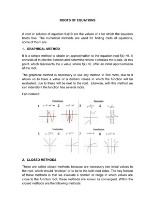
1. GRAPHICAL METHOD
It is a simple method to obtain an approximation to the equation root f(x) =0. It
consists of to plot the function and determine where it crosses the x-axis. At this
point, which represents the x value where f(x) =0, offer an initial approximation
of the root.
The graphical method is necessary to use any method to find roots, due to it
allows us to have a value or a domain values in which the function will be
evaluated, due to these will be next to the root. Likewise, with this method we
can indentify if the function has several roots.
For instance:
2. CLOSED METHODS
These are called closed methods because are necessary two initial values to
the root, which should “enclose” or to be to the both root sides. The key feature
of these methods is that we evaluate a domain or range in which values are
close to the function root; these methods are known as convergent. Within the
closed methods are the following methods:

2. 2.1. BISECTION(Also called Bolzano method)
The method feature lie in look for an interval where the function changes its sign
when is analyzed. The location of the sign change gets more accurately by
dividing the interval in a defined amount of sub-intervals. Each of this sub
intervals are evaluated to find the sign change. The approximation to the root
improves according to the sub-intervals are getting smaller.
The following is the procedure:
Step 1: Choose lower, xl, and upper, xu, values, which enclose the root, so that
the function changes sign in the interval. This is verified by checking that:
f  xl  f  xu   0
Step 2: An approximation of the xr root, is determined by:
xl  xu
xr 
2
Step 3: Realize the following evaluations to determine in what subinterval the
root is:
a. If f  xl  f  xr   0 , then the root is within the lower or left subinterval, so,
do xu=xr and return to step 2.
b. If f  xl  f  xr   0 , then the root is within the top or right subinterval, so,
do xl=xr and return to step 2.
c. If f  xl  f  xr   0 , the root is equal to xr; the calculations ends.

3. The maximum number of iterations to obtain the root value is given by the
following equation:
1 ������ − ������
������������ ����� =
ln⁡
(2) ������������������
TOL = Tolerance
2.2. THE METHOD OF FALSE POSITION
Although the bisection method is technically valid to determine roots, its focus is
relatively inefficient. Therefore this method is an improved alternative based on
an idea for a more efficient approach to the root.
This method raises draw a straight line joining the two interval points (x, y) and
(x1, y1), the cut generated by the x-axis allows greater approximation to the
root.
Using similar triangles, the intersection can be calculated as follows:
������(������1 ) ������(������2 )
=
������������ − ������������ ������������ − ������2
The final equation for False position method is:
������ ������2 (������1 − ������2 )
������������ = ������������ −
������ ������1 − ������(������2 )
The calculation of the root xr requires replacing one of the other two values so
that they always have opposite signs, what leads these two points always
enclose the root.
Sometimes, depending on the function, this method works poorly, while the
bisection method leads better approximations.

4. BIBLIOGRAPHY
CHAPRA, Steven C. y CANALE, Raymond P.: Métodos Numéricos para
Ingenieros. McGraw Hill 2007. 5ª edition.
http://www.numerical-methods.com/roots.htm