Download-manuals-surface water-waterlevel-29howtoestablishstagedischargeratingcurve

World Bank & Government of The Netherlands funded
Training module # SWDP - 29
How to establish stage
discharge rating curve
New Delhi, November 1999
CSMRS Building, 4th Floor, Olof Palme Marg, Hauz Khas,
New Delhi – 11 00 16 India
Tel: 68 61 681 / 84 Fax: (+ 91 11) 68 61 685
E-Mail: dhvdelft@del2.vsnl.net.in
DHV Consultants BV & DELFT HYDRAULICS
with
HALCROW, TAHAL, CES, ORG & JPS

HP Training Module File: “ 29 HOW TO ESTABLISH STAGE DISCHARGE RATING CURVE.DOC” Version Nov. 99
Page 1
Table of contents
Page
1. Module context 2
2. Module profile 3
3. Session plan 4
4. Overhead/flipchart master 7
5. Handout 8
6. Additional handout 10
7. Main text 11

Page 2
1. Module context
While designing a training course, the relationship between this module and the others,
would be maintained by keeping them close together in the syllabus and place them in a
logical sequence. The actual selection of the topics and the depth of training would, of
course, depend on the training needs of the participants, i.e. their knowledge level and skills
performance upon the start of the course.

Page 3
2. Module profile
Title : How to establish stage discharge rating curve
Target group :
Duration : x session of y min
Objectives : After the training the participants will be able to:
Key concepts : •
Training methods : Lecture, exercises
Training tools
required
: Board, flipchart
Handouts : As provided in this module
Further reading
and references
:

Page 4
3. Session plan
No Activities Time Tools
1 General
Overhead: Text: Establishing stage-discharge relation (1)
Overhead: Text: Establishing stage-discharge relation (2)
Overhead: Figure 1.1: Example rating curve
Overhead: Table 1.1 : Example rating curve computation output
10 min
OHS 1
OHS 2
OHS 3
OHS 4
2 The station control
Overhead: Text: The station control
Overhead: Text: Types of station controls
Overhead: Figure 2.1: Control configuration in natural channel
Overhead: Figure 2.2: Section control
Overhead: Figure 2.3: Channel control (1)
Overhead: Figure: Backwater effect
Overhead: Text: Channel control (2)
Overhead: Figure 2.4: Artificial control
Overhead: Text: Shifting controls
15 min
OHS 5
OHS 6
OHS 7
OHS 8
OHS 9
OHS 10
OHS 11
OHS 12
OHS 13
3
3.1
Fitting of rating curve
General
Overhead: Text: Fitting rating curves (1)
Overhead: Figure 3.1: Permanent control
Overhead: Figure 3.2a: Variable backwater (1)
Overhead: Figure 3.2b: Variable backwater (2)
Overhead: Figure 3.3: Unsteady flow
Overhead: Figure 3.4: River bed changes
Overhead: Figure 3.5: Effect of vegetation
120
min
OHS 14
OHS 15
OHS 16
OHS 17
OHS 18
OHS 19
OHS 20
OHS 21
OHS 22
3.2 Fitting of single channel rating curve
Overhead: Text: Fitting single channel simple rating curve (1)
Overhead: Figure 3.7 Trial and error procedure for a
Overhead: Text: Arithmetic procedure to determine a
Overhead: Text: Rating curve segments (1)
Overhead: Figure: Rating curve segments (2)
Overhead: Figure 3.6: Double logarithmic rating curve plot
Overhead: Text: Determination of rating curve coefficients (1)
Overhead: Figure 3.8: Example discharge rating curve Khed
Overhead: Table 3.1: Example output discharge rating Khed
120
min OHS 23
OHS 24
OHS 25
OHS 26
OHS 27
OHS 28
OHS 29
OHS 30
OHS 31
OHS 32
OHS 33
OHS 34
OHS 35
OHS 36
OHS 37
OHS 38
OHS 39
OHS 40

Page 5
Overhead: Text: Standard error of estimate in stage-discharge
relation
Overhead: Text: Uncertainty in rating curve fit
Overhead: Text: Confidence limits of rating curve
Overhead: Text: Fitting of rating curve in HYMOS
Exercise:
Develop rating curves for:
Chaskman and Khed for 1997
Rakshewa, Khamgaon and Pargaon (Bhima) for 1997 and
Continue with Dakor (Sabarmati) for 1991-97
OHS 41
OHS 42'
OHS 43
OHS 44
3.3 Compound channel rating curve
Overhead: Figure: Compound channel rating curve (1)
Overhead: Figure 3.10 Compound channel rating curve (2)
Overhead: Text: Compound channel rating curve (3)
Overhead: Text: Compound channel rating curve (4)
Overhead: Figure 3.11: Example rating curve compound
channel
60 min
OHS 45
OHS 46
OHS 47
OHS 48
OHS 49
3.4 Rating curve with backwater correction
Overhead: Text: Rating curve with backwater correction
Overhead: Figure: Backwater effect
Overhead: Text: Channel control
Overhead: Text: Backwater
Overhead: Text: Backwater correction (1)
Overhead: Text: Backwater correction (2)
Overhead: Text: Constant fall method
Overhead: Figure 3.12: Constant fall method
Overhead: Figure 3.13: Constant fall rating
Overhead: Constant fall computational procedure
Overhead: Normal fall method for backwater correction (1)
Overhead: Figure 3.14: Normal fall method for backwater
correction (2)
correction (3)
correction (4)
60 min
OHS 50
OHS 51
OHS 52
OHS 53
OHS 54
OHS 55
OHS 56
OHS 57
OHS 58
OHS 59
OHS 60
OHS 61
OHS 62
OHS 63
OHS 64
OHS 65
3.5 Rating curve with unsteady flow correction
Overhead: Rating curve with unsteady flow correction (1)
Overhead: Figure 3.15a: Example unsteady flow correction (1)
Overhead: Figure 3.15b: Example unsteady flow correction (1)
Overhead: Figure 3.15c: Example unsteady flow correction (1)
Overhead: Figure 3.15d: Example unsteady flow correction (1)
Overhead: Figure 3.15e: Example unsteady flow correction (1)
Exercise:
Apply manually the unsteady flow correction for station
Mahemdabad by:
60 min
OHS 66
OHS 67
OHS 68
OHS 69
OHS 70
OHS 71
OHS 72
OHS 73

Page 6
− assessing the river bed slope from the hydrographs at
NSB00I7 and Mahemdabad relative to MSL.
− estimating the celerity based on Manning's equation.
− determining the rise or fall rate from time derivative of
the hydrograph for stages > 28m + MSL
3.6 Rating relationships for stations affected by shifting
control
Overhead: Text: Shifting control (1)
Overhead: Figure 3.16: Shifting control (2), bed configurations
Overhead: Figure 3.17: Shifting control (3), indeterminate Q-h
Overhead: Figure 3.18: Shifting control (4), alternative: u-R plot
Overhead: Text: Shifting control (5), approaches
Overhead: Text: Shifting control (6), simple ratings between
events
Overhead: Text: Shifting control (7), varying shift parameter
Overhead: Text: Shifting control (8), Stout’s method (1)
Overhead: Figure 3.19: Shifting control (9), Stout’s method (2)
Overhead: Text: Shifting control (1), Stout’s method (3)
Overhead: Text: Shifting control (1), daily gauging
OHS 74
OHS 75
OHS 76
OHS 77
OHS 78
OHS 79
OHS 80
OHS 81
OHS 82
OHS 83
OHS 84

Page 7
4. Overhead/flipchart master

Page 8
5. Handout

Page 9
Add copy of Main text in chapter 8, for all participants.

Page 10
6. Additional handout
These handouts are distributed during delivery and contain test questions, answers to
questions, special worksheets, optional information, and other matters you would not like to
be seen in the regular handouts.
It is a good practice to pre-punch these additional handouts, so the participants can easily
insert them in the main handout folder.

Page 11
7. Main text
Contents
1. General 1
2. The station control 2
3. Fitting of rating curves 5

Page 1
How to establish stage discharge rating curve
1. General
• Flow is the variable usually required for hydrological analysis but, continuous
measurement of flow past a river section is usually impractical or prohibitively
expensive. However, stage can be observed continuously or at regular short time
intervals with comparative ease and economy. Fortunately, a relation exists
between stage and the corresponding discharge at river section. This relation is
termed a stage-discharge relationship or stage-discharge rating curve or simply,
rating curve.
• A rating curve is established by making a number of concurrent observations of
stage and discharge over a period of time covering the expected range of stages
at the river gauging section.
• At many locations, the discharge is not a unique function of stage; variables such
as surface slope or rate of change of stage with respect to time must also be
• known to obtain the complete relationship in such circumstances.
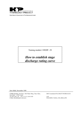
• The rating relationship thus established is used to transform the observed stages
into the corresponding discharges. In its simplest form, a rating curve can be
illustrated graphically, as shown in Figure 1.1, by the average curve fitting the scatter plot
between water level (as ordinate) and discharge (as abscissa) at any river section.
Figure 1.1 Example of stage-discharge rating curve
Rating curve Chaskman 1997
Rating Curve Measurements
Discharge (m3/s)
2,0001,9001,8001,7001,6001,5001,4001,3001,2001,1001,0009008007006005004003002001000
Waterlevel(m+MSL)
600
599
598
597
596
595
594

Page 2
• If Q and h are discharge and water level, then the relationship can be analytically
expressed as:
Q = f(h) (1)
Where; f(h) is an algebraic function of water level. A graphical stage discharge curve
helps in visualising the relationship and to transform stages manually to discharges
whereas an algebraic relationship can be advantageously used for analytical
transformation.
• Because it is difficult to measure flow at very high and low stages due to their
infrequent occurrence and also to the inherent difficulty of such measurements,
extrapolation is required to cover the full range of flows. Methods of extrapolation
are described in a later module.
2. The station control
• The shape, reliability and stability of the stage-discharge relation are controlled by
a section or reach of channel at or downstream from the gauging station and
known as the station control. The establishment and interpretation of stage discharge
relationships requires an understanding of the nature of controls and the types of control
at a particular station.
• Fitting of stage discharge relationships must not be considered simply a
mathematical exercise in curve fitting. Staff involved in fitting stage discharge
relationships should have familiarity with and experience of field hydrometrics.
The channel characteristics forming the control include the cross-sectional area and shape
of the stream channel, expansions and restrictions in the channel, channel sinuosity, the
stability and roughness of the streambed, and the vegetation cover all of which collectively
constitute the factors determining the channel conveyance.
2.1 Types of station control
The character of the rating curve depends on the type of control which in turn is
governed by the geometry of the cross section and by the physical features of the
river downstream of the section. Station controls are classified in a number of ways
as:
• section and channel controls
• natural and artificial controls
• complete, compound and partial controls
• permanent and shifting controls
2.1.1 Section and channel controls
When the control is such that any change in the physical characteristics of the channel
downstream to it has no effect on the flow at the gauging section itself then such control is
termed as section control. In other words, any disturbance downstream the control will not
be able to pass the control in the upstream direction. Natural or artificial local narrowing of
the cross-section (waterfalls, rock bar, gravel bar) creating a zone of acceleration are some
examples of section controls (Figs. 2.1 and 2.2). The section control necessarily has a
critical flow section at a short distance downstream.

Page 3
Figure 2.1 Example of section control
Figure 2.2 Example of section control. (low-water part
is sensitive, while high-water part is non-sensitive)
A cross section where no acceleration of flow occurs or where the acceleration is not
sufficient enough to prevent passage of disturbances from the downstream to the upstream
direction then such a location is called as a channel control. The rating curve in such case
depends upon the geometry and the roughness of the river downstream of the control (Fig.
2.3). The length of the downstream reach of the river affecting the rating curve depends on
the normal or equilibrium depth he and on the energy slope S (L ∝ he/S, where he follows
from Manning Q=KmBhe
5/3
S1/2
(wide rectangular channel) so he = (Q/KmS1/2
)3/5
). The length of
channel effective as a control increases with discharge. Generally, the flatter the stream
gradient, the longer the reach of channel control.

Page 4
Figure 2.3 Example of channel control
2.1.2 Artificial and natural controls
An artificial section control or structure control is one which has been specifically constructed
to stabilise the relationship between stage and discharge and for which a theoretical
relationship is available based on physical modelling. These include weirs and flumes,
discharging under free flow conditions (Fig. 5). Natural section controls include a ledge of
rock across a channel, the brink of a waterfall, or a local constriction in width (including
bridge openings). All channel controls are ‘natural’.
Figure 2.4 Example of an artificial control
2.1.3 Complete, compound and partial controls
Natural controls vary widely in geometry and stability. Some consist of a single topographical
feature such as a rock ledge across the channel at the crest of a rapid or waterfall so forming
a complete control. Such a complete control is one which governs the stage-discharge
relation throughout the entire range of stage experienced. However, in many cases, station
controls are a combination of section control at low stages and a channel control at high
stages and are thus called compound or complex controls. A partial control cases, station
controls are a combination of section control at low stages and a is one which operates over
a limited range of stage when a compound control is present, in the transition between
section and channel control. The section control begins to drown out with rising tailwater

Page 5
levels so that over a transitional range of stage the flow is dependent both on the elevation
and shape of the control and on the tailwater level.
2.1.4 Permanent and shifting controls
Where the geometry of a section and the resulting stage-discharge relationship does not
change with time, it is described as a stable or permanent control. Shifting controls change
with time and may be section controls such as boulder, gravel or sand riffles which undergo
periodic or near continuous scour and deposition, or they may be channel controls with
erodible bed and banks. Shifting controls thus typically result from:
• scour and fill in an unstable channel
• growth and decay of aquatic weeds
• overspilling and ponding in areas adjoining the stream channel.
The amount of gauging effort and maintenance cost to obtain a record of adequate
quality is much greater for shifting controls than for permanent controls. Since rating
curves for the unstable controls must be updated and/or validated at frequent intervals,
regular and frequent current meter measurements are required. In contrast, for stable
controls, the rating curve can be established once and needs validation only occasionally.
Since stage discharge observations require significant effort and money, it is always
preferred to select a gauging site with a section or structure control. However, this is not
practicable in many cases and one has to be content with either channel control or a
compound control.
3. Fitting of rating curves
3.1 General
A simple stage discharge relation is one where discharge depends upon stage only. A
complex rating curve occurs where additional variables such as the slope of the
energy line or the rate of change of stage with respect to time are required to define
the relationship. The need for a particular type of rating curve can be ascertained by first
plotting the observed stage and discharge data on a simple orthogonal plot. The scatter in
the plot gives a fairly good assessment of the type of stage-discharge relationship required
for the cross section. Examples of the scatter plots obtained for various conditions are
illustrated below.
If there is negligible scatter in the plotted points and it is possible to draw a smooth single
valued curve through the plotted points then a simple rating curve is required. This is shown
in Fig. 3.1.
Figure 3.1 Permanent control

Page 6
However, if scatter is not negligible then it requires further probing to determine the
cause of such higher scatter. There are four distinct possibilities:
• The station is affected by the variable backwater conditions arising due for example
to tidal influences or to high flows in a tributary joining downstream. In such cases, if the
plotted points are annotated with the corresponding slope of energy line (≈surface slope
for uniform flows) then a definite pattern can be observed. A smooth curve passing
through those points having normal slopes at various depths is drawn first. It can then be
seen that the points with greater variation in slopes from the corresponding normal
slopes are located farther from the curve. This is as shown in Fig. 3.2a and b.
• The stage discharge rating is affected by the variation in the local acceleration due
to unsteady flow. In such case, the plotted points can be annotated with the
corresponding rate of change of slope with respect to time. A smooth curve (steady state
curve) passing through those points having the least values of rate of change of stage is
drawn first. It can then be seen that all those points having positive values of rate of
change of stage are towards the right side of the curve and those with negative values
are towards the left of it. Also, the distance from the steady curve increases with the
increase in the magnitude of the rate of change of stage. This is as shown in Fig. 3.3.
Figure 3.3 Rating curve affected by
unsteady flow
Figure 3.2a Rating curve affected by
variable backwater (uniform channel)
Figure 3.2b Rating curve affected by
variable backwater (submergence of low-
water control)

Page 7
• The stage discharge rating is affected by scouring of the bed or changes in
vegetation characteristics. A shifting bed results in a wide scatter of points on the
graph. The changes are erratic and may be progressive or may fluctuate from scour in
one event and deposition in another. Examples are shown in Fig. 3.4.
Figure 3.4 Stage-discharge relation Figure 3.5 Stage-discharge relation
affected by scour and fill affected by vegetation growth
• If no suitable explanation can be given for the amount of scatter present in the
plot, then it can perhaps be attributed to the observational errors. Such errors can
occur due to non-standard procedures for stage discharge observations.
Thus, based on the interpretation of scatter of the stage discharge data, the
appropriate type of rating curve is fitted. There are four main cases:
• Simple rating curve: If simple stage discharge rating is warranted then either single
channel or compound channel rating curve is fitted according to whether the flow occur
essentially in the main channel or also extends to the flood plains.
• Rating curve with backwater corrections: If the stage discharge data is affected by
the backwater effect then the rating curve incorporating the backwater effects is to be
established. This requires additional information on the fall of stage with respect to an
auxiliary stage gauging station.
• Rating curve with unsteady flow correction: If the flows are affected by the
unsteadiness in the flow then the rating curve incorporating the unsteady flow effects is
established. This requires information on the rate of change of stage with respect to time
corresponding to each stage discharge data.
• Rating curve with shift adjustment: A rating curve with shift adjustment is warranted in
case the flows are affected by scouring and variable vegetation effects.
3.2 Fitting of single channel simple rating curve
Single channel simple rating curve is fitted in those circumstances when the flow is
contained the main channel section and can be assumed to be fairly steady. There is no
indication of any backwater affecting the relationship. The bed of the river also does not
significantly change so as create any shifts in the stage discharge relationship. The scatter
plot of the stage and discharge data shows a very little scatter if the observational errors are
not significant. The scatter plot of stage discharge data in such situations, typically is as

Page 8
shown in Fig. 1.1. The fitting of simple rating curves can conveniently be considered
under the following headings:
• equations used and their physical basis
• determination of datum correction(s)
• number and range of rating curve segments
• determination of rating curve coefficients
• estimation of uncertainty in the stage discharge relationship
3.2.1 Equations used and their physical basis
Two types of algebraic equations are commonly fitted to stage discharge data are:
1. Power type equation which is most commonly used:
(2)
2. Parabolic type of equation
(3)
where: Q = discharge (m3
/sec)
h = measured water level (m)
a = water level (m) corresponding to Q = 0
ci = coefficients derived for the relationship corresponding to the station
characteristics
It is anticipated that the power type equation is most frequently used in India and is
recommended. Taking logarithms of the power type equation results in a straight line
relationship of the form:
(4)
or
(5)
That is, if sets of discharge (Q) and the effective stage (h + a) are plotted on the double log
scale, they will represent a straight line. Coefficients A and B of the straight line fit are
functions of a and b. Since values of a and b can vary at different depths owing to changes
in physical characteristics (effective roughness and geometry) at different depths, one or
more straight lines will fit the data on double log plot. This is illustrated in Fig. 3.6, which
shows a distinct break in the nature of fit in two water level ranges. A plot of the cross
section at the gauging section is also often helpful to interpret the changes in the
characteristics at different levels.
)(log)(log)(log ahbcQ ++=
01
2
2 )()( cahcahcQ ww ++++=
XBAY +=
b
ahcQ )( +=

Page 9
Figure 3.6 Double logarithmic
plot of rating curve showing a
distict break
The relationship between rating curve parameters and physical conditions is also
evident if the power and parabolic equations are compared with Manning’s equation
for determining discharges in steady flow situations. The Manning’s equation can be
given as:
Q
n
AR S
n
S AR
function of roughness slope depth geometry
m = =
=
1 12 3 1 2 1 2 2 3/ / / /
( )( )
( & ) & ( & )
(6)
Hence, the coefficients a, c and d are some measures of roughness and geometry of the
control and b is a measure of the geometry of the section at various depths. The value of
coefficient b for various geometrical shapes are as follows:
For rectangular shape: about 1.6
For triangular shape : about 2.5
For parabolic shape : about 2.0
For irregular shape : 1.6 to 1.9
Changes in the channel resistance and slope with stage, however, will affect the exponent b.
The net result of these factors is that the exponent for relatively wide rivers with channel
control will vary from about 1.3 to 1.8. For relatively deep narrow rivers with section control,
the exponent will commonly be greater than 2 and sometimes exceed a value of 3. Note that
for compound channels with flow over the floodplain or braided channels over a limited
range of level, very high values of the exponent are sometimes found (>5).
3.2.2 Determination of datum correction (a)
The datum correction (a) corresponds to that value of water level for which the flow is
zero. From eq. (2) it can be seen that for Q = 0, (h + a) = 0 which means:
a = -h.
Physically, this level corresponds to the zero flow condition at the control effective at the
measuring section. The exact location of the effective control is easily determined for
artificial controls or where the control is well defined by a rock ledge forming a section
control. For the channel controlled gauging station, the level of deepest point opposite the
gauge may give a reasonable indication of datum correction. In some cases identification of
the datum correction may be impractical especially where the control is compound and
channel control shifts progressively downstream at higher flows. Note that the datum
correction may change between different controls and different segments of the rating curve.

Page 10
For upper segments the datum correction is effectively the level of zero flow had that control
applied down to zero flow; it is thus a nominal value and not physically ascertainable.
Alternative analytical methods of assessing “a” are therefore commonly used and
methods for estimating the datum correction are as follows:
• trial and error procedure
• arithmetic procedure
• computer-based optimisation
However, where possible, the estimates should be verified during field visits and inspection
of longitudinal and cross sectional profiles at the measuring section:
Trial and error procedure
This was the method most commonly used before the advent of computer-based methods.
The stage discharge observations are plotted on double log plot and a median line fitted
through them. This fitted line usually is a curved line. However, as explained above, if the
stages are adjusted for zero flow condition, i.e. datum correction a, then this line should be a
straight line. This is achieved by taking a trial value of “a” and plotting (h + a), the adjusted
stage, and discharge data on the same double log plot. It can be seen that if the unadjusted
stage discharge plot is concave downwards then a positive trial value of “a” is needed to
make it a straight line. And conversely, a negative trial value is needed to make the line
straight if the curve is concave upwards. A few values of “a” can be tried to attain a straight
line fit for the plotted points of adjusted stage discharge data. The procedure is illustrated in
Fig.3.7. This procedure was slow but quite effective when done earlier manually. However,
making use of general spreadsheet software (having graphical provision) for such trial and
error procedure can be very convenient and faster now.
Figure 3.7 Determination of
datum correction (a) by trial and
error
Arithmetic procedure:
This procedure is based on expressing the datum correction “a” in terms of observed water
levels. This is possible by way elimination of coefficients b and c from the power type
equation between gauge and discharge using simple mathematical manipulation. From the
median curve fitting the stage discharge observations, two points are selected in the lower
and upper range (Q1 and Q3) whereas the third point Q2 is computed from Q2
2
=Q1.Q3,
such that:
(7)
3
2
2
1
Q
Q
Q
Q
=

Page 11
If the corresponding gauge heights for these discharges read from the plot are h1, h2 and h3
then using the power type, we obtain:
(8)
Which yields:
(9)
From this equation an estimated value of “a” can be obtained directly. This procedure is
known as Johnson method which is described in the WMO Operational Hydrology manual
on stream gauging (Report No. 13, 1980).
.
Optimisation procedure:
This procedure is suitable for automatic data processing using computer and “a” is obtained
by optimisation. The first trial value of the datum correction “a” is either input by the user
based on the field survey or from the computerised Johnson method described above. Next,
this first estimate of “a” is varied within 2 m so as to obtain a minimum mean square error in
the fit. This is a purely mathematical procedure and probably gives the best results on the
basis of observed stage discharge data but it is important to make sure that the result is
confirmed where possible by physical explanation of the control at the gauging location. The
procedure is repeated for each segment of the rating curve.
3.2.3 Number and ranges of rating curve segments:
After the datum correction “a” has been established, the next step is to determine if the rating
curve is composed of one or more segments. This is normally selected by the user rather
than done automatically by computer. It is done by plotting the adjusted stage, (h-a) or
simply “h” where there are multiple segments, and discharge data on the double log scale.
This scatter plot can be drawn manually or by computer and the plot is inspected for
breaking points. Since for (h-a), on double log scale the plotted points will align as straight
lines, breaks are readily identified. The value of “h” at the breaking points give the first
estimate of the water levels at which changes in the nature of the rating curve are expected.
The number and water level ranges for which different rating curves are to be established is
thus noted. For example, Fig. 3.6 shows that two separate rating curves are required for the
two ranges of water level – one up to level “h1” and second from “h1” onwards. The rating
equation for each of these segments is then established and the breaking points between
segments are checked by computer analysis (See below).
3.2.4 Determination of rating curve coefficients:
A least square method is normally employed for estimating the rating curve
coefficients. For example, for the power type equation, taking αα and ββ as the estimates
of the constants of the straight line fitted to the scatter of points in double log scale,
the estimated value of the logarithm of the discharge can be obtained as:
(10)
The least square method minimises the sum of square of deviations between the
logarithms of measured discharges and the estimated discharges obtained from the
fitted rating curve. Considering the sum of square the error as E, we can write:
(11)
)(
)(
)(
)(
3
2
2
1
ahc
ahc
ahc
ahc
+
+
=
+
+
231
31
2
2
2hhh
hhh
a
−+
−
=
XY βα +=ˆ
2
1
2
1
)()ˆ( i
N
i
ii
N
i
i XYYYE βα −−=−= ∑∑
==

Page 12
Here i denotes the individual observed point and N is the total number of observed stage
discharge data.
Since this error is to be minimum, the slope of partial derivatives of this error with respect to
the constants must be zero. In other words:
(12)
and
(13)
This results in two algebraic equations of the form:
(14)
and
(15)
All the quantities in the above equations are known except α and β. Solving the two
equations yield:
(16)
and
(17)
The value of coefficients c and b of power type equation can then be finally obtained as:
b = β and c = 10α
(18)
Reassessment of breaking points
The first estimate of the water level ranges for different segments of the rating curve is
obtained by visual examination of the cross-section changes and the double log plot.
However, exact limits of water levels for various segments are obtained by computer from
the intersection of the fitted curves in adjoining the segments.
0
})({ 2
1
=
∂
−−∂
=
∂
∂
∑=
α
βα
α
i
N
i
i XY
E
0
})({ 2
1
=
∂
−−∂
=
∂
∂
∑
=
β
βα
β
i
N
i
i XY
E
0
11
=−− ∑∑
==
N
i
i
N
i
i XNY βα
0)()( 2
111
=−− ∑∑∑
===
N
i
i
N
i
i
N
i
ii XXYX βα
N
XY
N
i
i
N
i
i ∑∑ ==
−
= 11
β
α
∑ ∑
∑ ∑ ∑
= =
= = =
−
−
= N
i
N
i
ii
N
i
N
i
N
i
iiii
XXN
YXYXN
1 1
22
1 1 1
)()(
)()()(
β

Page 13
Considering the rating equations for two successive water level ranges be given as Q
= fi-1(h) and Q = fi (h) respectively and let the upper boundary used for the estimation of fi-1
be denoted by hui-1 and the lower boundary used for the estimation of fi by hli . To force the
intersection between fi-1 and fi to fall within certain limits it is necessary to choose: hui-1 > hli .
That is, the intersection of the rating curves of the adjoining segments should be found
numerically within this overlap. This is illustrated in Fig. 3.8 and Table 3.1. If the intersection
falls outside the selected overlap, then the intersection is estimated for the least difference
between Q = fi-1(h) and Q = fi (h). Preferably the boundary width between hui-1 and hli is
widened and the curves refitted.
It is essential that a graphical plot of the fit of the derived equations to the data is inspected
before accepting them.
Figure 3.8 Fitted
rating curve using 2
segments
3.2.5 Estimation of uncertainty in the stage discharge relationship:
With respect to the stage discharge relationship the standard error of estimate (Se) is
a measure of the dispersion of observations about the mean relationship. The
standard error is expressed as:
(19)
Here, ∆Qi is the measure of difference between the observed (Qi) and computed (Qc)
discharges and can be expressed in absolute and relative (percentage) terms respectively
as:
(20)
or
(21)
2
)( 2
−
∆−∆
=
∑
N
QQ
S
i
e
cii QQQ −=∆
%100×
−
=∆
i
ci
i
Q
QQ
Q
Rating Curve KHED 23/8/97 - 31/10/97
Rating Curve Measurements
Discharge (m3/s)
1,8001,6001,4001,2001,0008006004002000
Wa
ter
Le
vel
(m
+M
SL)
590
589
588
587
586
585
584
583

Page 14
Table 3.1 Results of stage-discharge computation for example presented in Figure 3.8
Analysis of stage-discharge data
Station name : KHED
Data from 1997 1 1 to 1997 12 31
Single channel
Gauge Zero on 1997 7 30 = .000 m
Number of data = 36
h minimum = 583.79 meas.nr = 44
h maximum = 589.75 meas.nr = 49
q minimum = 20.630 meas.nr = 44
q maximum = 1854.496 meas.nr = 49
Given boundaries for computation of rating curve(s)
interval lower bound upper bound nr. of data
1 583.000 587.000 31
2 586.500 590.000 6
Power type of equation q=c*(h+a)**b is used
Boundaries / coefficients
lower bound upper bound a b c
583.00 586.68 -583.650 1.074 .1709E+03
586.68 590.00 -581.964 2.381 .1401E+02
Number W level Q meas Q comp DIFf Rel.dIFf Semr
M M3/S M3/S M3/S 0/0 0/0
2 584.610 181.500 163.549 17.951 10.98 3.08
3 587.390 768.820 785.226 -16.406 -2.09 3.54
5 586.240 457.050 475.121 -18.071 -3.80 4.93
6 585.870 386.020 402.597 -16.577 -4.12 4.60
7 585.440 316.290 319.452 -3.162 -.99 4.16
9 585.210 261.650 275.570 -13.920 -5.05 3.89
10 584.840 200.850 206.013 -5.163 -2.51 3.41
………………………………………………………………………………………………………………………………………………………………………
48 583.870 32.490 33.574 -1.084 -3.23 3.35
49 589.750 1854.496 1854.988 -.492 -.03 6.02
50 588.470 1228.290 1209.632 18.658 1.54 3.48
51 587.270 753.580 744.518 9.062 1.22 3.79
52 587.120 673.660 695.381 -21.721 -3.12 4.14
53 586.600 553.930 546.431 7.499 1.37 5.21
54 586.320 509.230 490.911 18.319 3.73 4.99
55 585.620 357.030 354.093 2.937 .83 4.35
56 585.410 319.860 313.697 6.163 1.96 4.12
57 584.870 226.080 211.593 14.487 6.85 3.45
62 584.040 59.020 62.120 -3.100 -4.99 2.69
Overall standard error = 6.603
Statistics per interval
Interval Lower bound Upper bound Nr.of data Standard error
1 583.000 586.680 31 7.11
2 586.680 590.000 5 2.45

Page 15
Standard error expressed in relative terms helps in comparing the extent of fit
between the rating curves for different ranges of discharges. The standard error for the
rating curve can be derived for each segment separately as well as for the full range of data.
Thus 95% of all observed stage discharge data are expected to be within t x Se from the
fitted line where:
Student’s t ≅ 2 where n > 20, but increasingly large for smaller samples.
The stage discharge relationship, being a line of best fit provides a better estimate of
discharge than any of the individual observations, but the position of the line is also
subject to uncertainty, expressed as the Standard error of the mean relationship (Smr)
which is given by:
(22)
where t = Student t-value at 95% probability
Pi = ln (hi + a)
S2
P = variance of P
CL 95% = 95% confidence limits
The Se equation gives a single value for the standard error of the logarithmic relation and the
95% confidence limits can thus be displayed as two parallel straight lines on either side of
the mean relationship. By contrast Smr is calculated for each observation of (h + a). The
limits are therefore curved on each side of the stage discharge relationship and are at a
minimum at the mean value of ln (h + a) where the Smr relationship reduces to:
Smr = ± Se / n1/2
(23)
Thus with n = 25, Smr, the standard error of the mean relationship is approximately
20% of Se indicating the advantage of a fitted relationship over the use of individual
gaugings.
3.3 Compound channel rating curve
If the flood plains carry flow over the full cross section, the discharge (for very wide
channels) consists of two parts:
)()( 2/13/2
ShKBhQ mrrriver = (24)
and
])([)()(
2/13/2
11 ShhKBBhhQ mfrfloodplain −−−= (25)
mr
P
i
emr tSCLand
S
PP
n
SS ±=
−
+= %95
2
2
)(1

Page 16
assuming that the floodplain has the same slope as the river bed, the total discharge
becomes:
(26)
This is illustrated in Fig. 3.9. The rating curve changes significantly as soon as the flood plain
at level h-h1 is flooded, especially if the ratio of the storage width B to the width of the river
bed Br is large. The rating curve for this situation of a compound channel is
determined by considering the flow through the floodplain portion separately. This is
done to avoid large values of the exponent b and extremely low values for the
parameter c in the power equation for the rating curve in the main channel portion.
Figure 3.9 Example of
rating curve for compound
cross-section
The last water level range considered for fitting rating curve is treated for the flood plain
water levels. First, the river discharge Qr will be computed for this last interval by using the
parameters computed for the one but last interval. Then a temporary flood plain discharge Qf
is computed by subtracting Qr from the observed discharge (Oobs) for the last water level
interval, i.e.
Qf = Qobs - Qr. (27)
This discharge Qf will then be separately used to fit a rating curve for the water levels
corresponding to the flood plains. The total discharge in the flood plain is then calculated as
the sum of discharges given by the rating curve of the one but last segment applied for water
levels in the flood plains and the rating curve established separately for the flood plains.
The rating curve presented in Figure 3.9 for Jhelum river at Rasul reads:
For h < 215.67 m + MSL: Q = 315.2(h-212.38)1.706
For h > 215.67 m + MSL: Q = 315.2(h-212.38)1.706
+ 3337.4(h-215.67)1.145
])([)()()( 2/13/2
11
2/13/2
ShhKBBhhShKBhQ mfrmrrtotal −−−+=

Page 17
Hence the last part in the second equation is the contribution of the flood plain to the total
river flow.
3.4 Rating curve with backwater correction
When the control at the gauging station is influenced by other controls downstream,
then the unique relationship between stage and discharge at the gauging station is
not maintained. Backwater is an important consideration in streamflow site selection and
sites having backwater effects should be avoided if possible. However, many existing
stations in India are subject to variable backwater effects and require special methods of
discharge determination. Typical examples of backwater effects on gauging stations
and the rating curve are as follows:
• by regulation of water course downstream.
• level of water in the main river at the confluence downstream
• level of water in a reservoir downstream
• variable tidal effect occurring downstream of a gauging station
• downstream constriction with a variable capacity at any level due to weed growth etc.
• rivers with return of overbank flow
Backwater from variable controls downstream from the station influences the water surface
slope at the station for given stage. When the backwater from the downstream control
results in lowering the water surface slope, a smaller discharge passes through the gauging
station for the same stage. On the other hand, if the surface slope increases, as in the case
of sudden drawdown through a regulator downstream, a greater discharge passes for the
same stage. The presence of backwater does not allow the use of a simple unique rating
curve. Variable backwater causes a variable energy slope for the same stage.
Discharge is thus a function of both stage and slope and the relation is termed as
slope-stage-discharge relation.
The stage is measured continuously at the main gauging station. The slope is
estimated by continuously observing the stage at an additional gauge station, called
the auxiliary gauge station. The auxiliary gauge station is established some distance
downstream of the main station. Time synchronisation in the observations at the gauges is
necessary for precise estimation of slope. The distance between these gauges is kept such
that it gives an adequate representation of the slope at the main station and at the same
time the uncertainty in the estimation is also smaller. When both main and auxiliary gauges
are set to the same datum, the difference between the two stages directly gives the fall in the
water surface. Thus, the fall between the main and the auxiliary stations is taken as the
measure of surface slope. This fall is taken as the third parameter in the relationship
and the rating is therefore also called stage-fall-discharge relation.
Discharge using Manning’s equation can be expressed as:
(28)
Energy slope represented by the surface water slope can be represented by the fall in level
between the main gauge and the auxiliary gauge. The slope-stage-discharge or stage-
fall-discharge method is represented by:
(29)
ASRKQ m
2/13/2
=
p
r
m
p
r
m
r
m
F
F
S
S
Q
Q






=





=

Page 18
where Qm is the measured (backwater affected) discharge
Qr is a reference discharge
Fm is the measured fall
Fr is a reference fall
p is a power parameter between 0.4 and 0.6
From the Manning’s equation given above, the exponent “p” would be expected to be ½. The
fall (F) or the slope (S = F/L) is obtained by the observing the water levels at the main and
auxiliary gauge. Since, there is no assurance that the water surface profile between these
gauges is a straight line, the effective value of the exponent can be different from ½ and
must be determined empirically.
An initial plot of the stage discharge relationship (either manually or by computer) with
values of fall against each observation, will show whether the relationship is affected by
variable slope, and whether this occurs at all stages or is affected only when the fall reduces
below a particular value. In the absence of any channel control, the discharge would be
affected by variable fall at all times and the correction is applied by the constant fall
method. When the discharge is affected only when the fall reduces below a given value the
normal (or limiting) fall method is used.
3.4.1 Constant fall method:
The constant fall method is applied when the stage-discharge relation is affected by variable
fall at all times and for all stages. The fall applicable to each discharge measurement is
determined and plotted with each stage discharge observation on the plot. If the observed
falls do not vary greatly, an average value (reference fall or constant fall) Fr is selected.
Manual computation
For manual computation an iterative graphical procedure is used. Two curves are
used (Figs. 3.10 and 3.11):
• All measurements with fall of about Fr are fitted with a curve as a simple stage discharge
relation (Fig.3.10). This gives a relation between the measured stage h and the
reference discharge Qr.
• A second relation, called the adjustment curve, either between the measured fall, Fm, or
the ratio of the measured fall for each gauging and the constant fall (Fm / Fr), and the
discharge ratio (Qm / Qr) (Fig. 3.11)
• This second curve is then used to refine the stage discharge relationship by calculating
Qr from known values of Qm and Fm/Fr and then replotting h against Qr .
• A few iterations may be done to refine the two curves.

Page 19
Figure 3.10 Qr=f(h) in constant fall rating Figure 3.11 Qm/Qr = f(Fm/Fr)
The discharge at any time can be then be computed as follows:
• For the observed fall (Fm) calculate the ratio (Fm/Fr)
• read the ratio (Qm / Qr) from the adjustment curve against the calculated value of (Fm/Fr)
• multiply the ratio (Qm / Qr) with the reference discharge Qr obtained for the measured
stage h from the curve between stage h and reference discharge Qr.
Computer computation
For computer computation, this procedure is simplified by mathematical fitting and
optimisation. First, as before, a reference (or constant) fall (Fr) is selected from
amongst the most frequently observed falls.
A rating curve, between stage h and the reference discharge (Qr), is then fitted directly
by estimating:
(30)
where p is optimised between 0.4 and 0.6 based on minimisation of standard errors.
The discharge at any time, corresponding to the measured stage h and fall Fm , is then
calculated by first obtaining Qr from the above relationship and then calculating
discharge as:
(31)
A special case of constant fall method is the unit fall method in which the reference fall is
assumed to be equal to unity. This simplifies the calculations and thus is suitable for manual
method.
p
m
r
mr
F
F
QQ 





=
p
r
m
r
F
F
QQ 





=

Page 20
3.4.2 Normal Fall Method:
The normal or limiting fall method is used when there are times when backwater is not
present at the station. Examples are when a downstream reservoir is drawn down or
where there is low water in a downstream tributary or main river.
Manual procedure
The manual procedure is as follows:
• Plot stage against discharge, noting the fall at each point. The points at which backwater
has no effect are identified first. These points normally group at the extreme right of the
plotted points. This is equivalent to the simple rating curve for which a Qr -h relationship
may be fitted (where Qr in this case is the reference or normal discharge) (Fig. 3.12).
Figure 3.12 Qr-h relationship
for Normal Fall Method
• Plot the measured fall against stage for each gauging and draw a line through those
observations representing the minimum fall, but which are backwater free. This
represents the normal or limiting fall Fr (Fig. 3.13). It is observed from Figure 3.13 that
the line separates the backwater affected and backwater free falls.
Figure 3.13 Fr-h relationship

Page 21
• For each discharge measurement derive Qr using the discharge rating and Fr , the
normal fall from the fall rating.
• For each discharge measurement compute Qm/Qr and Fm/Fr and draw an average curve
(Fig. 3.14).
Figure 3.14 Qm/Qr - Fm/Fr
relationship
• As for the constant fall method, the curves may be successively adjusted by holding two
graphs constant and re-computing and plotting the third. No more than two or three
iterations are usually required.
The discharge at any time can be then be computed as follows:
• From the plot between stage and the normal (or limiting) fall (Fr), find the value of Fr for
the observed stage h
• For the observed fall (Fm), calculate the ratio (Fm/Fr)
• Read the ratio (Qm / Qr) from the adjustment curve against the calculated value of
(Fm/Fr)
• Obtain discharge by multiplying the ratio (Qm / Qr) with the reference discharge Qr
obtained for the measured stage h from the curve between stage h and reference
discharge Qr.
Computer procedure
The computer procedure considerably simplifies computation and is as follows:
• Compute the backwater-free rating curve using selected current meter gaugings (the Qr
-h relationship).
• Using values of Qr derived from (1) and Fr derived from:
(32)
a parabola is fitted to the reference fall in relation to stage (h) as:
(33)
The parameter p is optimised between 0.4 and 0.6.
p
m
r
mr
Q
Q
FF
/1






=
2
hchbaFr ++=

Page 22
The discharge at any time, corresponding to the measured stage h and fall Fm , is then
calculated by:
• obtaining Fr for the observed h from the parabolic relation between h and Fr
• obtaining Qr from the backwater free relationship established between h and Qr
• then calculating discharge corresponding to measured stage h as:
(34)
3.5 Rating curve with unsteady flow correction
Gauging stations not subjected to variable slope because of backwater may still be
affected by variations in the water surface slope due to high rates of change in stage.
This occurs when the flow is highly unsteady and the water level is changing rapidly. At
stream gauging stations located in a reach where the slope is very flat, the stage-discharge
relation is frequently affected by the superimposed slope of the rising and falling limb of the
passing flood wave. During the rising stage, the velocity and discharge are normally greater
than they would be for the same stage under steady flow conditions. Similarly, during the
falling stage the discharge is normally less for any given gauge height than it is when the
stage is constant. This is due to the fact that the approaching velocities in the advancing
portion of the wave are larger than in a steady uniform flow at the corresponding stages. In
the receding phase of the flood wave the converse situation occurs with reduced approach
velocities giving lower discharges than in equivalent steady state case.
Thus, the stage discharge relationship for an unsteady flow will not be a single-valued
relationship as in steady flow but it will be a looped curve as shown in the example below.
The looping in the stage discharge curve is also called hysteresis in the stage-discharge
relationship. From the curve it can be easily seen that at the same stage, more discharge
passes through the river during rising stages than in the falling ones.
3.5.1 Application
For practical purposes the discharge rating must be developed by the application of
adjustment factors that relate unsteady flow to steady flow. Omitting the acceleration
terms in the dynamic flow equation the relation between the unsteady and steady
discharge is expressed in the form:
(35)
where Qm is measured discharge
Qr is estimated steady state discharge from the rating curve
c is wave velocity (celerity)
S0 is energy slope for steady state flow
dh/dt is rate of change of stage derived from the difference in gauge
height at the beginning and end of a gauging (+ for rising ; - for
falling)
Qr is the steady state discharge and is obtained by establishing a rating curve as a median
curve through the uncorrected stage discharge observations or using those observations for
which the rate of change of stage had been negligible. Care is taken to see that there are
p
r
m
r
F
F
QQ 





=








+=
dt
dh
Sc
QQ rm
0
1
1

Page 23
sufficient number of gaugings on rising and falling limbs if the unsteady state observations
are considered while establishing the steady state rating curve.
Rearranging the above equation gives:
(36)
The quantity (dh/dt) is obtained by knowing the stage at the beginning and end of the stage
discharge observation or from the continuous stage record. Thus the value of factor (1/cS0)
can be obtained by the above relationship for every observed stage. The factor (1/cS0)
varies with stage and a parabola is fitted to its estimated values and stage as:
(37)
A minimum stage hmin is specified beyond which the above relation is valid. A maximum
value of factor (1/cS0) is also specified so that unacceptably high value can be avoided from
taking part in the fitting of the parabola.
Thus unsteady flow corrections can be estimated by the following steps:
• Measured discharge is plotted against stage and beside each plotted point is noted the
value of dh/dt for the measurement (+ or - )
• A trial Qs rating curve representing the steady flow condition where dh/dt equals zero is
fitted to the plotted discharge measurements.
• A steady state discharge Qr is then estimated from the curve for each discharge
measurement and Qm , Qr and dh/dt are together used in the Equation 35 to compute
corresponding values of the adjustment factor 1 / cS0
• Computed values of 1 / cS0 are then plotted against stage and a smooth (parabolic)
curve is fitted to the plotted points
For obtaining unsteady flow discharge from the steady rating curve the following steps are
followed:
• obtain the steady state flow Qr for the measured stage h
• obtain factor (1/cS0) by substituting stage h in the parabolic relation between the two
• obtain (dh/dt) from stage discharge observation timings or continuous stage records
• substitute the above three quantities in the Equation 35 to obtain the true unsteady flow
discharge
The computer method of analysis using HYMOS mirrors the manual method described
above.
It is apparent from the above discussions and relationships that the effects of
unsteady flow on the rating are mainly observed in larger rivers with very flat bed
slopes (with channel control extending far downstream) together with significant rate
change in the flow rates. For rivers with steep slopes, the looping effect is rarely of
practical consequence. Although there will be variations depending on the catchment
climate and topography, the potential effects of rapidly changing discharge on the
rating should be investigated in rivers with a slope of 1 metre/ km or less. Possibility
of a significant unsteady effect (say more than 8–10%) can be judged easily by
making a rough estimate of ratio of unsteady flow value with that of the steady flow
value.
dtdh
QQ
Sc
rm
/
1)/(1
2
0
−
=
2
0
1
chhba
Sc
++=

Page 24
Example
The steps to correct the rating curve for unsteady flow effects is elaborated for station
MAHEMDABAD on WAZAK river. The scatter plot of stage discharge data for 1997 is shown
in Figure 3.15a. From the curve is apparent that some shift has taken place, see also Figure
3.15b. The shift took place around 24 August.
Figure 3.15a Stage-discharge data of station Figure 3.15 b Detail of stage
Mahemdabad on Wazak river, 1997 discharge data for low flows, clearly
showing the shift
In the analysis therefore only the data prior that date were considered. The scatter plots
clearly show a looping for the higher flows. To a large extent, this looping can be attributed
to unsteady flow phenomenon. The Jones method is therefore applied. The first fit to the
scatter plot, before any correction, is shown in Figure 3.15c.
Figure 3.15c First fit to stage-
discharge data, prior to
adjustment
Based on this relation and the observed discharges and water level changes values for
1/cS0 were obtained. These data are depicted in Figure 3.15d. The scatter in the latter plot is
seen to be considerable. An approximate relationship between 1/cS0 and h is shown in the
graph.

Page 25
Figure 3.15 d Scatter plot
of 1/cS0 as function of
stage, with approximate
relation.
With the values for 1/cS0 taken from graph the unsteady flow correction factor is computed
and steady state discharges are computed. These are shown in Figure 3.15e, together with
the uncorrected discharges. It is observed that part of the earlier variation is indeed
removed. A slightly adjusted curve is subsequently fit to the stage and corrected flows.
Figure 3.15e Rating curve
after first adjustment trial
for unsteady flow.
Note that the looping has been eliminated, though still some scatter is apparent.

Page 26
3.6 Rating relationships for stations affected by shifting control
For site selection it is a desirable property of a gauging station to have a control
which is stable, but no such conditions may exist in the reach for which flow
measurement is required, and the selected gauging station may be subject to shifting
control. Shifts in the control occur especially in alluvial sand-bed streams. However, even in
stable stream channels shift will occur, particularly at low flow because of weed growth in the
channel, or as a result of debris caught in the control section.
In alluvial sand-bed streams, the stage-discharge relation usually changes with time,
either gradually or abruptly, due to scour and silting in the channel and because of
moving sand dunes and bars. The extent and frequency with which changes occur
depends on typical bed material size at the control and velocities typically occurring
at the station. In the case of controls consisting of cobble or boulder sized alluvium, the
control and hence the rating may change only during the highest floods. In contrast, in sand
bed rivers the control may shift gradually even in low to moderate flows. Intermediate
conditions are common where the bed and rating change frequently during the monsoon but
remain stable for long periods of seasonal recession.
For sand bed channels the stage-discharge relationship varies not only because of the
changing cross section due to scouring or deposition but also because of changing
roughness with different bed forms. Bed configurations occurring with increasing discharge
are ripples, dunes, plane bed, standing waves, antidunes and chute and pool (Fig. 3.16).
The resistance of flow is greatest in the dunes range. When the dunes are washed out and
the sand is rearranged to form a plane bed, there is a marked decrease in bed roughness
and resistance to the flow causing an abrupt discontinuity in the stage-discharge relation.
Fine sediment present in water also influences the configuration of sand-bed and thus the
resistance to flow. Changes in water temperature may also alter bed form, and hence
roughness and resistance to flow in sand bed channels. The viscosity of water will increase
with lower temperature and thereby mobility of the sand will increase.

Page 27
Figure 3.16 Bed and surface configurations configurations in sand-bed channels
For alluvial streams where neither bottom nor sides are stable, a plot of stage against
discharge will very often scatter widely and thus be indeterminate (Fig. 3.17) However, the
hydraulic relationship becomes apparent by changing the variables. The effect of variation in
bottom elevation and width is eliminated by replacing stage by mean depth (hydraulic radius)
and discharge by mean velocity respectively. Plots of mean depth against mean velocity are
useful in the analysis of stage-discharge relations, provided the measurements are referred
to the same cross-section.

Page 28
Figure 3.17 Plot of discharge against stage for a sand-bed
channel with indeterminate stage-discharge relation
These plots will identify the bed-form regime associated with each individual discharge
measurement. (Fig. 3.18). Thus measurements associated with respective flow regimes,
upper or lower, are considered for establishing separate rating curves. Information about
bed-forms may be obtained by visual observation of water surfaces and noted for reference
for developing discharge ratings.
Figure 3.18 Relation of mean velocity to
hydraulic radius of channel in Figure 3.17
There are four possible approaches depending on the severity of scour and on the
frequency of gauging:
• Fitting a simple rating curve between scour events
• Varying the zero or shift parameter
• Application of Stout’s shift method
• Flow determined from daily gauging

Page 29
3.6.1 Fitting a simple rating curve between scour events
Where the plotted rating curve shows long periods of stability punctuated by infrequent flood
events which cause channel adjustments, the standard procedure of fitting a simple
logarithmic equation of the form Q = c1(h + a1)b1
should be applied to each stable period.
This is possible only if there are sufficient gaugings in each period throughout the range of
stage.
To identify the date of change from one rating to the next, the gaugings are plotted with their
date or number sequence. The interval in which the change occurred is where the position of
sequential plotted gaugings moves from one line to the next. The processor should then
inspect the gauge observation record for a flood event during the period and apply the next
rating from that date.
Notes from the Field Record book or station log must be available whilst inspection and
stage discharge processing is carried out. This provides further information on the nature
and timing of the event and confirms that the change was due to shifting control rather than
to damage or adjustment to the staff gauge.
3.6.2 Varying the zero or shift parameter
Where the plotted rating curve shows periods of stability but the number of gaugings
is insufficient to define the new relationship over all or part of the range, then the
parameter ‘a’ in the standard relationship Q = c1(h + a1 )b1
may be adjusted. The
parameter ‘a1’ represents the datum correction between the zero of the gauges and the
stage at zero flow. Scour or deposition causes a shift in this zero flow stage and hence a
change in the value ‘a1’..
The shift adjustment required can be determined by taking the average difference (∆a)
between the rated stage (hr) for measured flow (Qm) and measured stage (hm) using the
previous rating. i.e.
∆a h h nr
i
n
m= −
=
∑( ) /
1
(39)
The new rating over the specified range then becomes:
Q = c1(h + a1 + ∆a)b1
(40)
The judgement of the processor is required as to whether to apply the value of ∆a over the
full range of stage (given that the % effect will diminish with increasing stage) or only in the
lower range for which current meter gauging is available. If there is evidence that the rating
changes from unstable section control at low flows to more stable channel control at higher
flows, then the existing upper rating should continue to apply.
New stage ranges and limits between rating segments will require to be determined. The
method assumes that the channel hydraulic properties remain unchanged except for the
level of the datum. Significant variation from this assumption will result in wide variation in (hr
- hm) between included gaugings. If this is the case then Stout’s shift method should be used
as an alternative.

Page 30
3.6.3 Stout’s shift method (Not Recommended to be Applied )
For controls which are shifting continually or progressively, Stout’s method is used. In such
instances the plotted current meter measurements show a very wide spread from the mean
line and show an insufficient number of sequential gaugings with the same trend to split the
simple rating into several periods. The procedure is as follows:
• Fit a mean relationship to (all) the points for the period in question.
• Determine hr (the rated stage) from measured Qm by reversing the power type rating
curve or from the plot:
hr = (Qm / c)1/b
- a (41)
• Individual rating shifts (∆h), as shown in Fig. 3.19, are then:
∆h = hr - hm (42)
• These ∆h stage shifts are then plotted chronologically and interpolated between
successive gaugings (Fig. 3.19) for any instant of time t as ∆ht.
• These shifts, ∆ht ,are used as a correction to observed gauge height readings and the
original rating applied to the corrected stages, i.e.
Qt = c1(ht +∆ht + a1)b1
(43)
Figure 3.19 Stout’s method for correcting stage readings when control is shifting
The Stout method will only result in worthwhile results where:
(a) Gauging is frequent, perhaps daily in moderate to high flows and even more frequently
during floods.
(b) The mean rating is revised periodically - at least yearly.
The basic assumption in applying the Stout’s method is that the deviations of the measured
discharges from the established stage-discharge curve are due only to a change or shift in
the station control, and that the corrections applied to the observed gauge heights vary
gradually and systematically between the days on which the check measurements are taken.
However, the deviation of a discharge measurement from an established rating curve may
be due to:

Page 31
(a) gradual and systematic shifts in the control,
(b) abrupt random shifts in the control, and
(c) error of observation and systematic errors of both instrumental and a personnel nature.
Stout’s method is strictly appropriate for making adjustments for the first type of error only. If
the check measurements are taken frequently enough, fair adjustments may be made for the
second type of error also. The drawback of the Stout’s method is that all the errors in
current meter observation are mixed with the errors due to shift in control and are
thus incorporated in the final estimates of discharge. The Stout method must
therefore never be used where the rating is stable, or at least sufficiently stable to
develop satisfactory rating curves between major shift events; use of the Stout
method in such circumstances loses the advantage of a fitted line where the standard
error of the line Smr is 20% of the standard error of individual gaugings (Se). Also,
when significant observational errors are expected to be present it is strongly
recommended not to apply this method for establishing the rating curve.
3.6.4 Flow determined from daily gauging
Stations occur where there is a very broad scatter in the rating relationship, which appears
neither to result from backwater or scour and where the calculated shift is erratic. A cause
may be the irregular opening and closure of a valve or gate in a downstream structure.
Unless there is a desperate need for such data, it is recommended that the station be moved
or closed. If the station is continued, a daily measured discharge may be adopted as the
daily mean flow. This practice however eliminates the daily variations and peaks in the
record.
It is emphasised that even using the recommended methods, the accuracy of flow
determination at stations which are affected by shifting control will be much less than at
stations not so affected. Additionally, the cost of obtaining worthwhile data will be
considerably higher. At many such stations uncertainties of ± 20 to 30% are the best that
can be achieved and consideration should be given to whether such accuracy meets the
functional needs of the station.

Download-manuals-surface water-waterlevel-29howtoestablishstagedischargeratingcurve

Recommended

Recommended

More Related Content

What's hot

What's hot (20)

Viewers also liked

Viewers also liked (13)

Similar to Download-manuals-surface water-waterlevel-29howtoestablishstagedischargeratingcurve

Similar to Download-manuals-surface water-waterlevel-29howtoestablishstagedischargeratingcurve (20)

More from hydrologyproject001

More from hydrologyproject001 (20)

Recently uploaded

Recently uploaded (20)

Download-manuals-surface water-waterlevel-29howtoestablishstagedischargeratingcurve