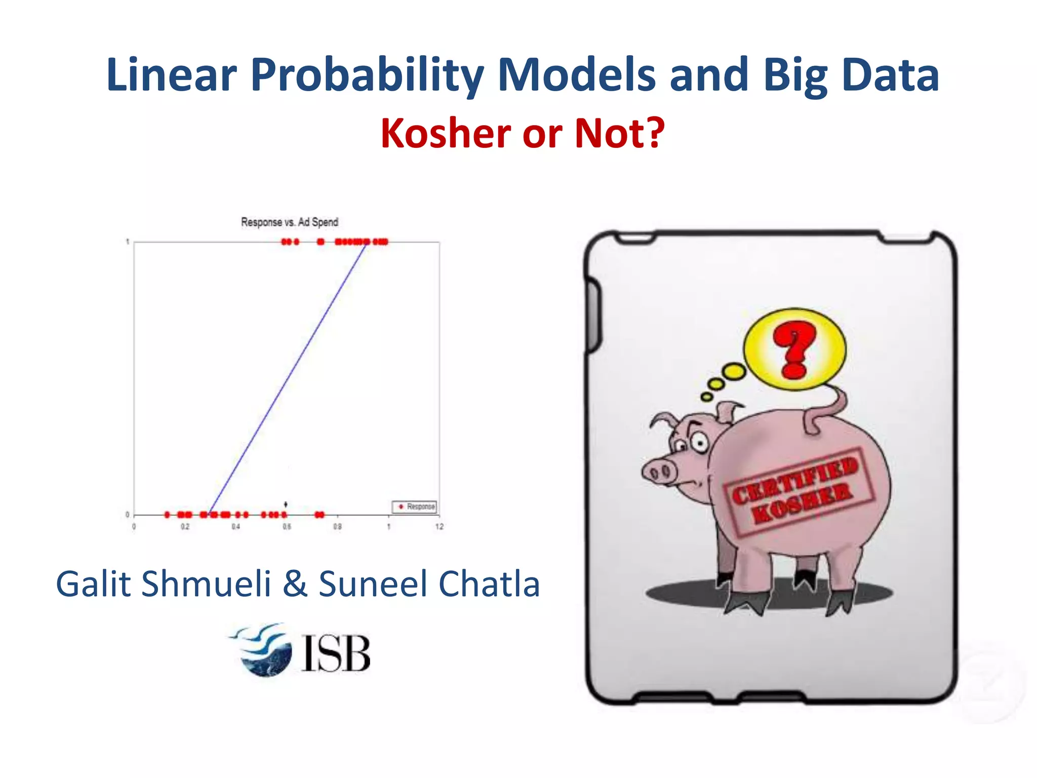
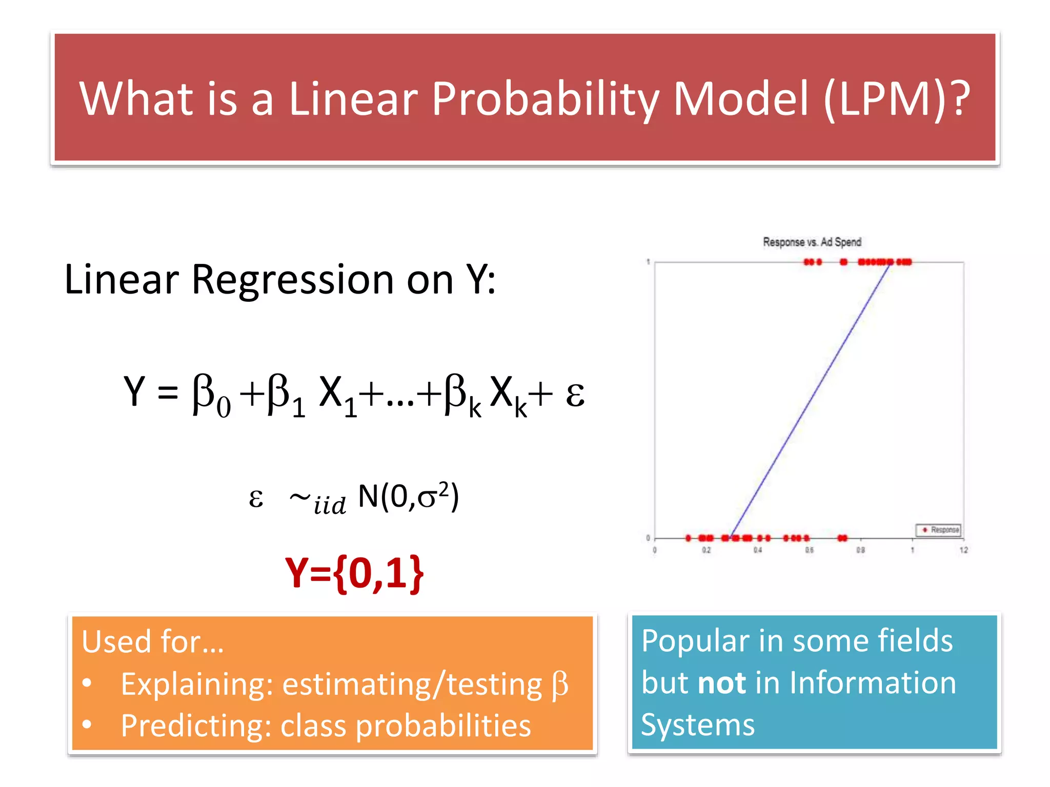
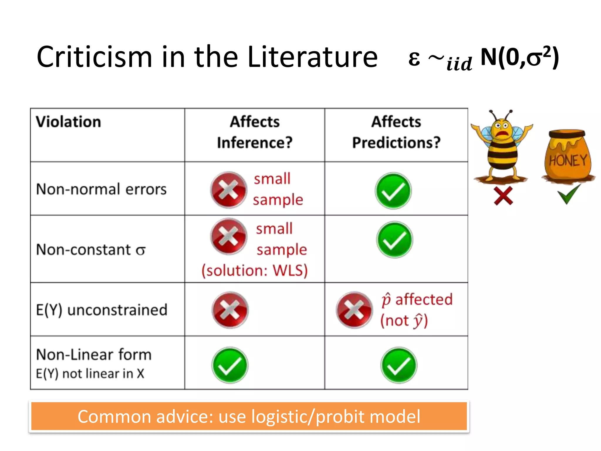
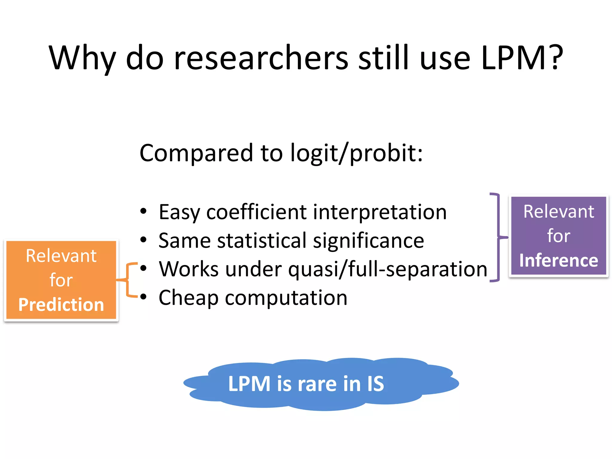
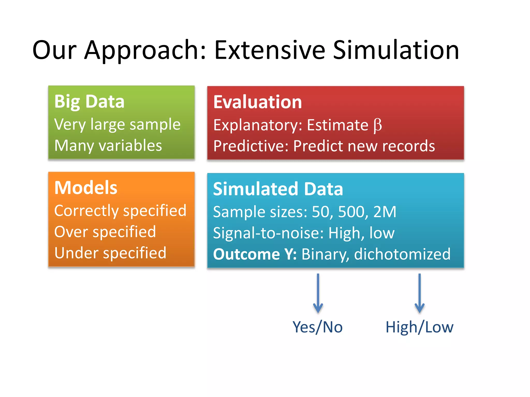
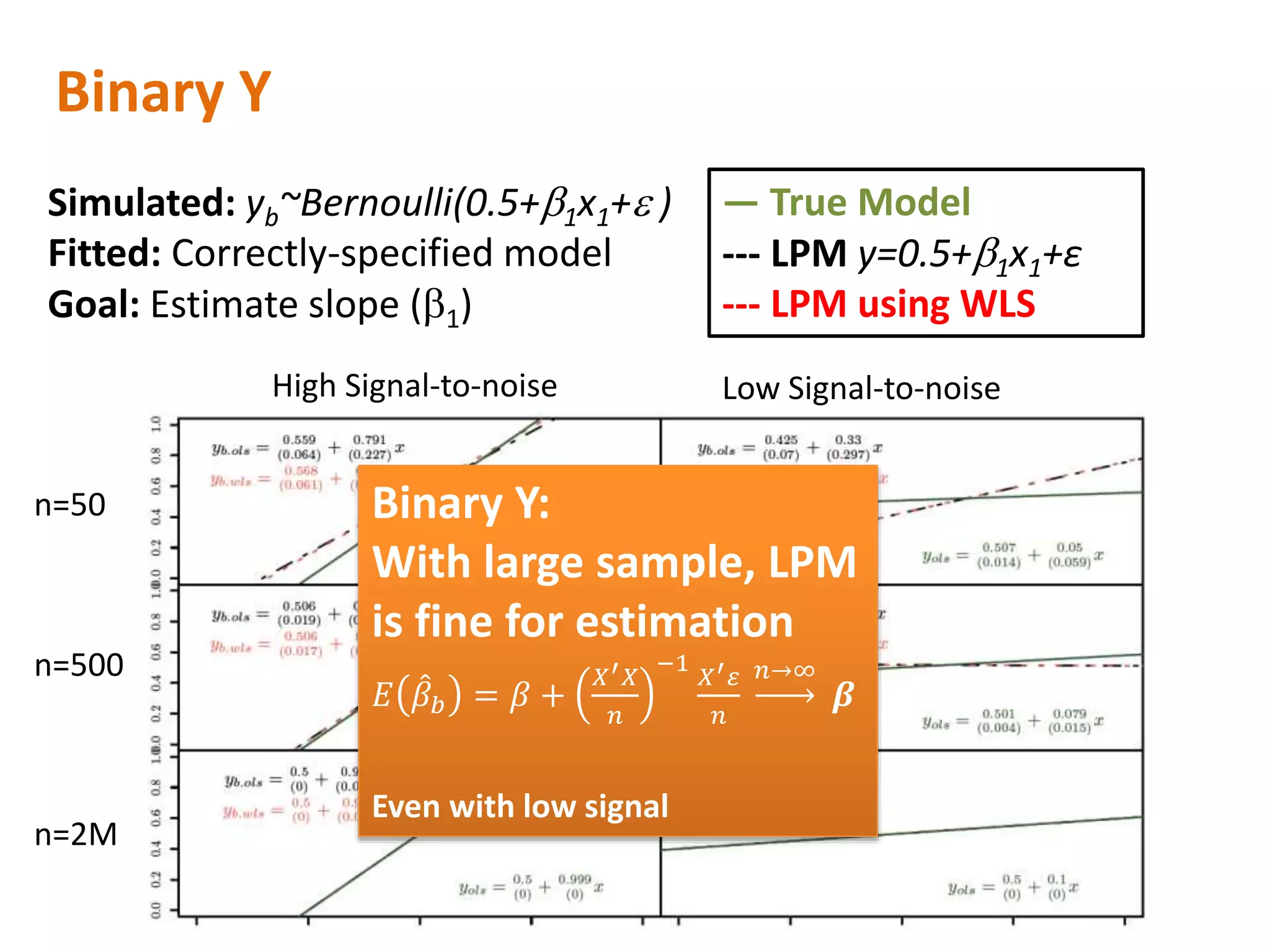
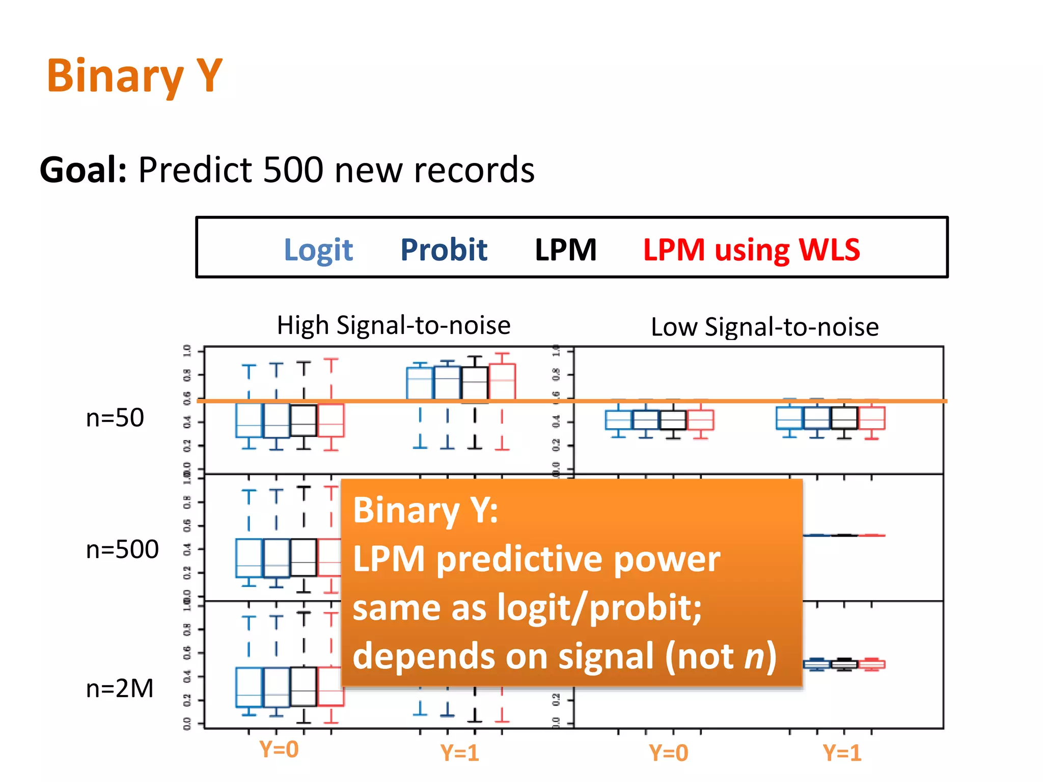
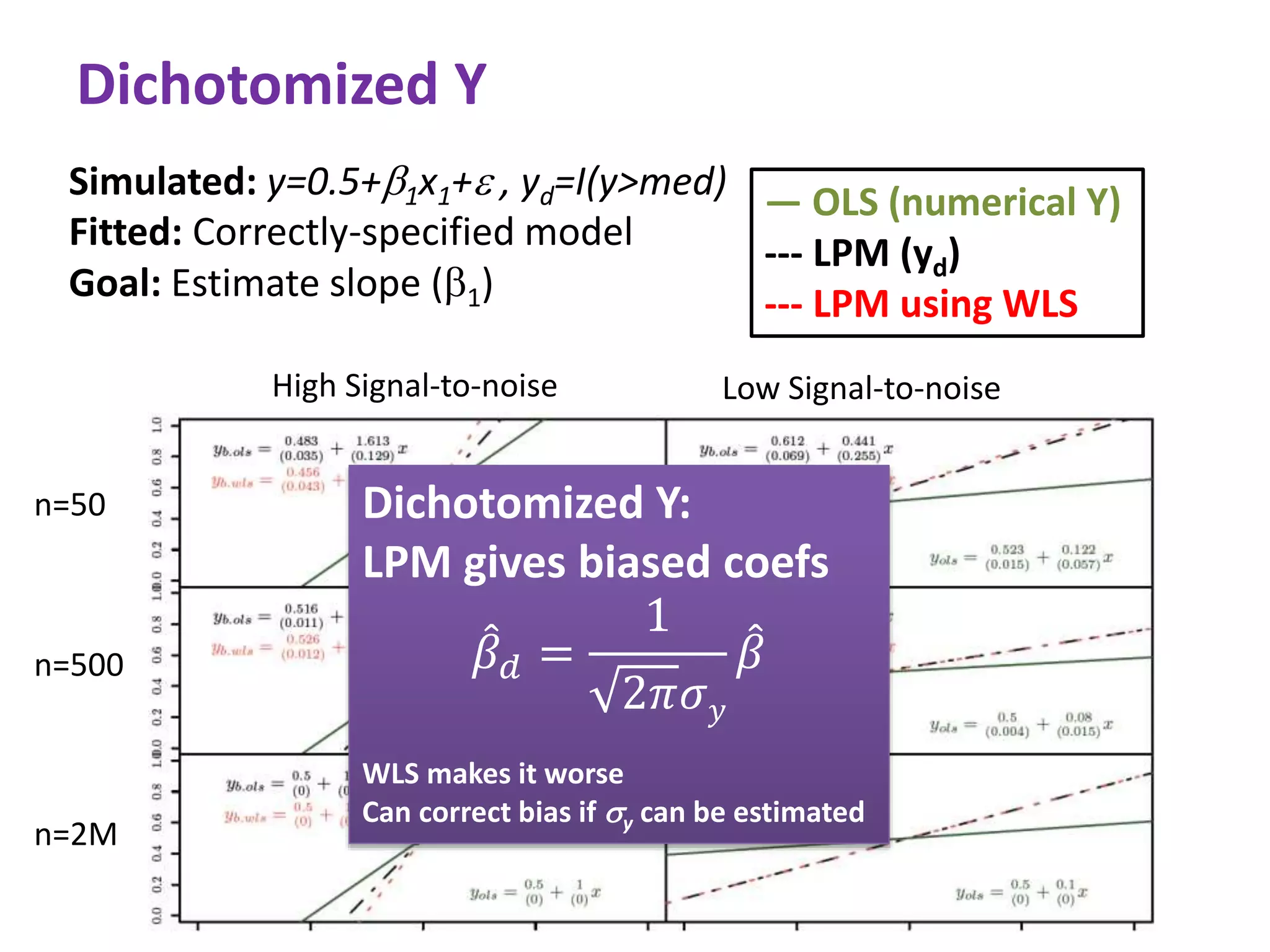
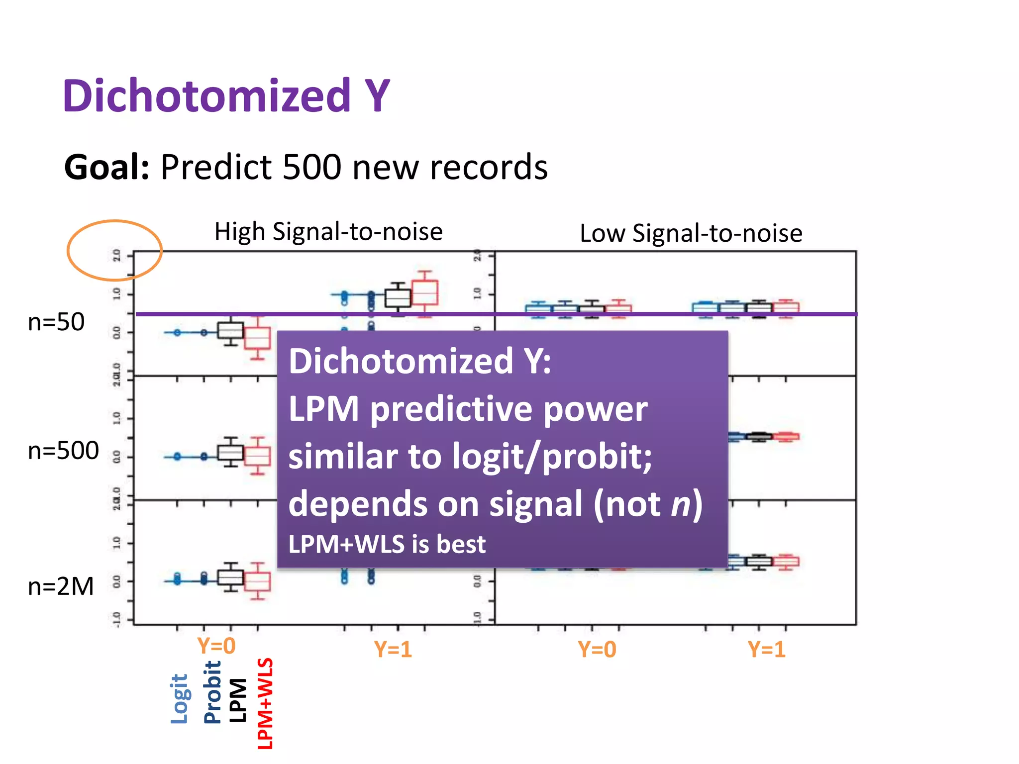
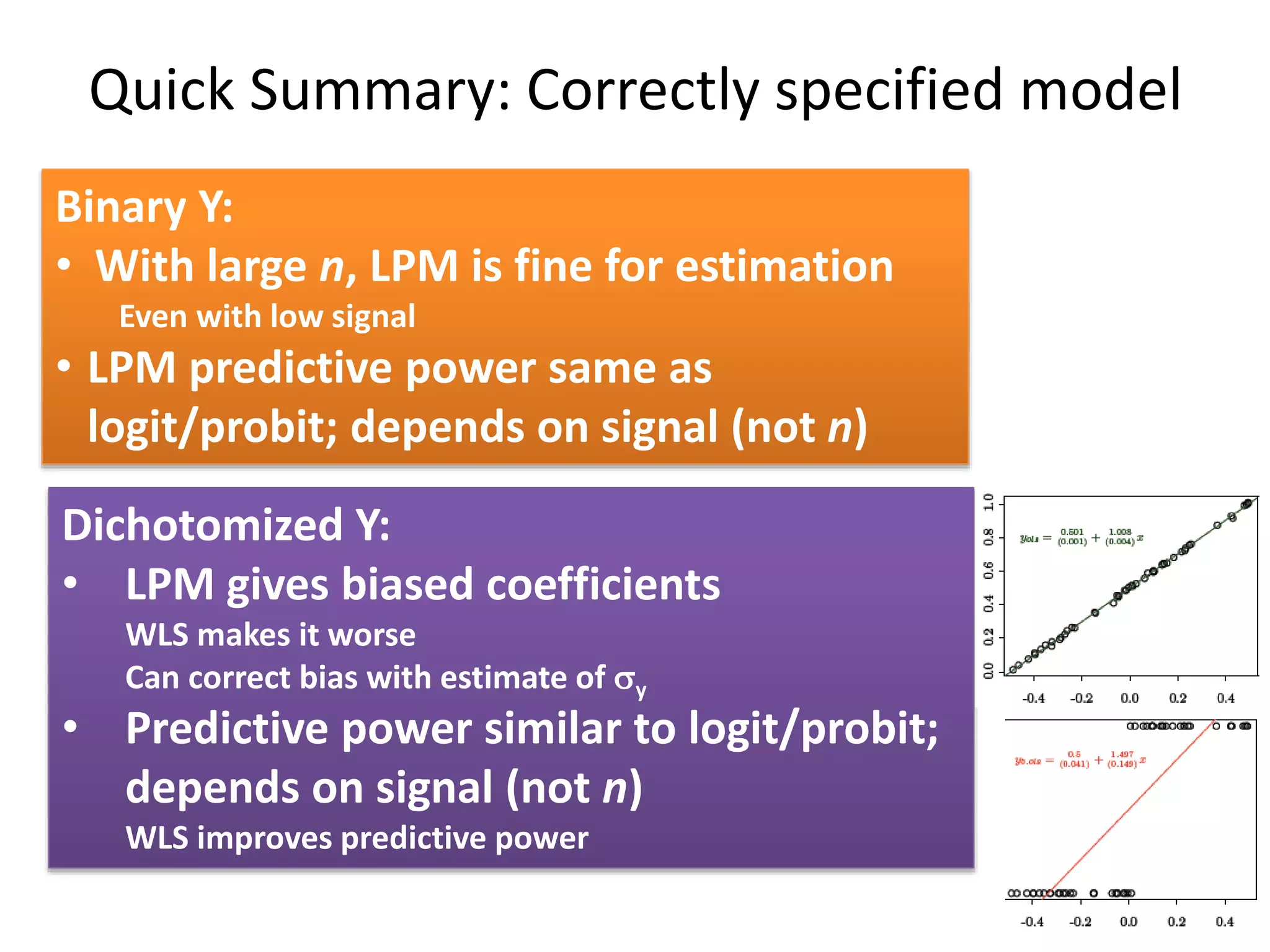
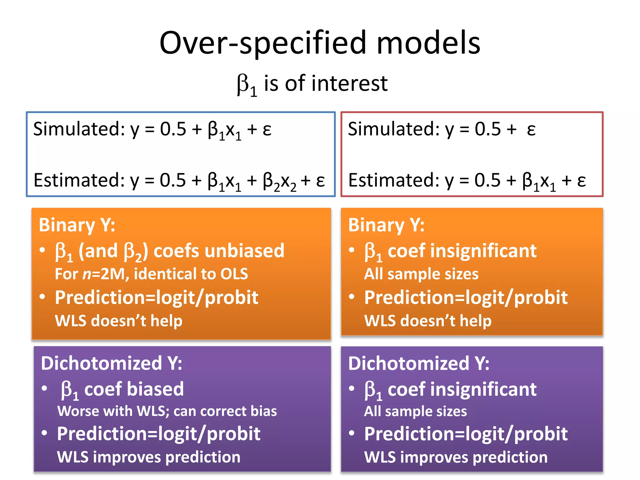
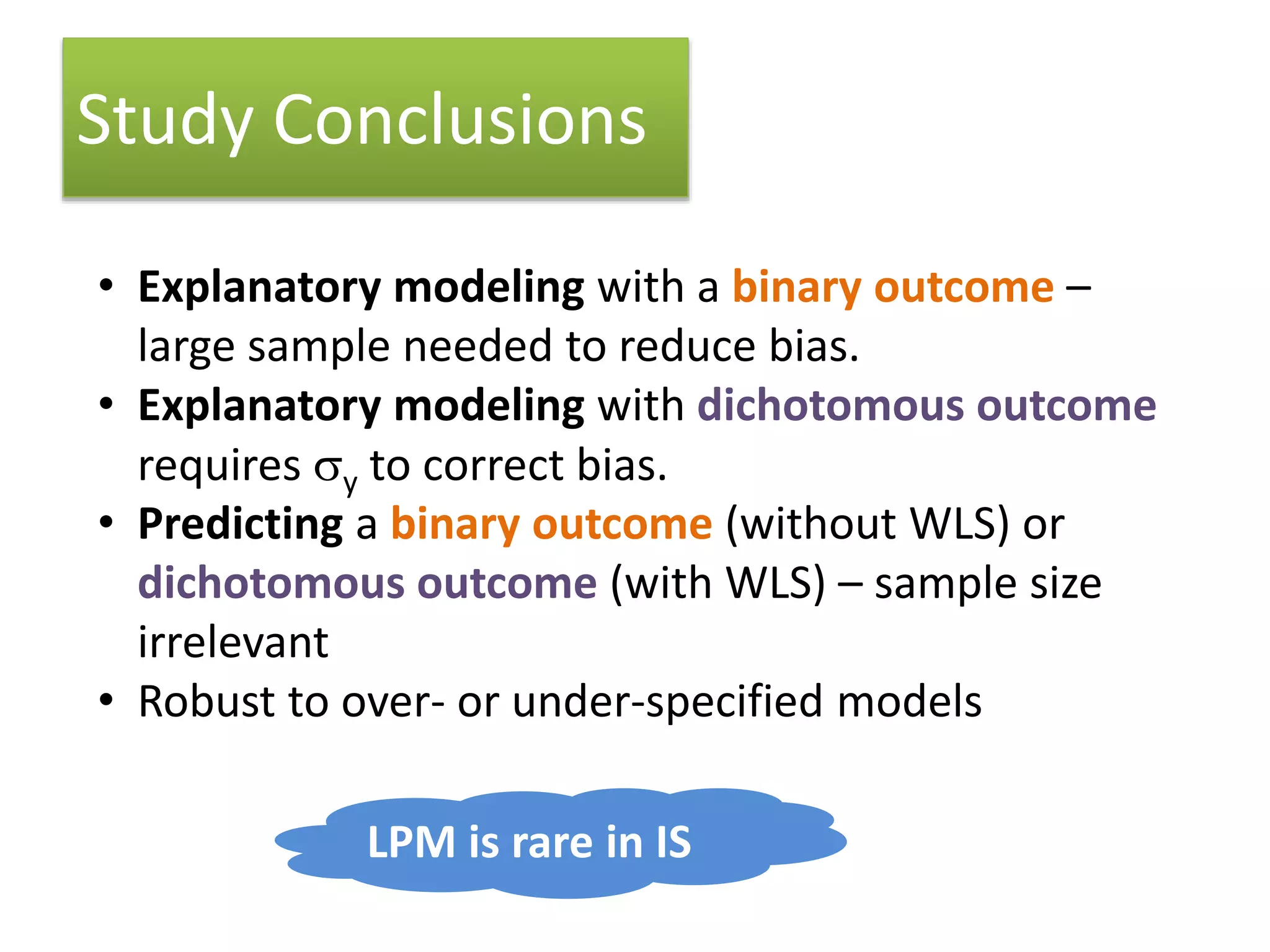
Slides from Galit Shmueli's talk at the 10th Statistical Challenges in eCommerce Research (SCECR) symposium, Tel Aviv, Israel. http://scecr.org/scecr2014/

1. Linear Probability Models and Big Data
Kosher or Not?
Galit Shmueli & Suneel Chatla

2. Linear Regression on Y:
Y = b0 +b1 X1+…+bk Xk+ e
e ~𝑖𝑖𝑑 N(0,s2)
Y={0,1}
What is a Linear Probability Model (LPM)?
Used for…
• Explaining: estimating/testing b
• Predicting: class probabilities
Popular in some fields
but not in Information
Systems

3. Criticism in the Literature e ~𝒊𝒊𝒅 N(0,s2)
Common advice: use logistic/probit model

4. Why do researchers still use LPM?
Compared to logit/probit:
• Easy coefficient interpretation
• Same statistical significance
• Works under quasi/full-separation
• Cheap computation
Relevant
for
InferenceRelevant
for
Prediction
LPM is rare in IS

5. Should we use LPM?

6. Our Approach: Extensive Simulation
Evaluation
Explanatory: Estimate b
Predictive: Predict new records
Big Data
Very large sample
Many variables
Models
Correctly specified
Over specified
Under specified
Simulated Data
Sample sizes: 50, 500, 2M
Signal-to-noise: High, low
Outcome Y: Binary, dichotomized
Yes/No High/Low

7. Study Design
Covariates:
X ~ U(-0.5,0.5)
e ~ N(0,s2)
Simulation Models:
y = 0.5 + β1x1 + ε
y = 0.5 + ε
y = 0.5 + β1x1 + β2x2 + ε
Signal-to-noise:
High: s=0.01, β1=1, (β2=0.01)
Low: s=0.10, β1=0.10, (β2=0.45)
Outcome Origin:
Binary: yb ~ Bernoulli (y)
Dichotomized: yd = I(y ≥ median(y))
Estimated Models:
y = 0.5 + β1x1 + ε
y = 0.5 + β1x1 + β2x2 + ε
Prediction:
n=500 holdout sample
Logit and Probit models

8. Binary Y
High Signal-to-noise Low Signal-to-noise
n=50
n=500
n=2M
— True Model
--- LPM y=0.5+b1x1+ε
--- LPM using WLS
Simulated: yb~Bernoulli(0.5+b1x1+e )
Fitted: Correctly-specified model
Goal: Estimate slope (b1)
Binary Y:
With large sample, LPM
is fine for estimation
𝐸 𝛽 𝑏 = 𝛽 +
𝑋′ 𝑋
𝑛
−1
𝑋′ 𝜀
𝑛
𝑛→∞
𝜷
Even with low signal

9. High Signal-to-noise Low Signal-to-noise
n=50
n=500
n=2M
Y=0 Y=0Y=1 Y=1
Binary Y:
LPM predictive power
same as logit/probit;
depends on signal (not n)
Binary Y
Goal: Predict 500 new records
Logit Probit LPM LPM using WLS

10. Dichotomized Y
High Signal-to-noise Low Signal-to-noise
n=50
n=500
n=2M
— OLS (numerical Y)
--- LPM (yd)
--- LPM using WLS
Dichotomized Y:
LPM gives biased coefs
𝛽 𝑑 =
1
2𝜋𝜎 𝑦
𝛽
WLS makes it worse
Can correct bias if sy can be estimated
Simulated: y=0.5+b1x1+e , yd=I(y>med)
Fitted: Correctly-specified model
Goal: Estimate slope (b1)

11. Dichotomized Y
High Signal-to-noise Low Signal-to-noise
n=50
n=500
n=2M
Logit
Probit
LPM
LPM+WLS
Y=0 Y=0Y=1 Y=1
Dichotomized Y:
LPM predictive power
similar to logit/probit;
depends on signal (not n)
LPM+WLS is best
Goal: Predict 500 new records

12. Dichotomized Y:
• LPM gives biased coefficients
WLS makes it worse
Can correct bias with estimate of sy
• Predictive power similar to logit/probit;
depends on signal (not n)
WLS improves predictive power
Quick Summary: Correctly specified model
Binary Y:
• With large n, LPM is fine for estimation
Even with low signal
• LPM predictive power same as
logit/probit; depends on signal (not n)

13. Over-specified models
b1 is of interest
Simulated: y = 0.5 + β1x1 + ε
Estimated: y = 0.5 + β1x1 + β2x2 + ε
Simulated: y = 0.5 + ε
Estimated: y = 0.5 + β1x1 + ε
Binary Y:
• b1 coef insignificant
All sample sizes
• Prediction=logit/probit
WLS doesn’t help
Binary Y:
• b1 (and b2) coefs unbiased
For n=2M, identical to OLS
• Prediction=logit/probit
WLS doesn’t help
Dichotomized Y:
• b1 coef insignificant
All sample sizes
• Prediction=logit/probit
WLS improves prediction
Dichotomized Y:
• b1 coef biased
Worse with WLS; can correct bias
• Prediction=logit/probit
WLS improves prediction

14. Modeling Auction Price
300,000 eBay auctions (Aug 2007- Jan 2008)
Price = f(min_bid, duration, seller_feedback, reserve)
1. Estimation/inference: determinants of price
2. Prediction: holdout sample (n = 5,000)
Dichotomized
Price

15. Inference/Estimation
Sample so large: all coefficients significant!
Bias due to dichotomization - corrected

16. Prediction
Removal of outliers gives identical ROC curves

17. Study Conclusions
• Explanatory modeling with a binary outcome –
large sample needed to reduce bias.
• Explanatory modeling with dichotomous outcome
requires sy to correct bias.
• Predicting a binary outcome (without WLS) or
dichotomous outcome (with WLS) – sample size
irrelevant
• Robust to over- or under-specified models
LPM is rare in IS