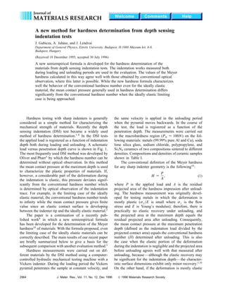
1. Journal of
Welcome Comments Help
MATERIALS RESEARCH
A new method for hardness determination from depth sensing
indentation tests
J. Gubicza, A. Juh´ sz, and J. Lendvai
a
Department of General Physics, E¨ tv¨ s University, Budapest, H-1088 M´
o o uzeum krt. 6-8,
Budapest, Hungary
(Received 18 December 1995; accepted 30 July 1996)
A new semiempirical formula is developed for the hardness determination of the
materials from depth sensing indentation tests. The indentation works measured both
during loading and unloading periods are used in the evaluation. The values of the Meyer
hardness calculated in this way agree well with those obtained by conventional optical
observation, where this latter is possible. While the new hardness formula characterizes
well the behavior of the conventional hardness number even for the ideally elastic
material, the mean contact pressure generally used in hardness determination differs
significantly from the conventional hardness number when the ideally elastic limiting
case is being approached.
Hardness testing with sharp indenters is generally the same velocity is applied in the unloading period
considered as a simple method for characterizing the when the pyramid moves backwards. In the course of
mechanical strength of materials. Recently the depth the test, the load is registered as a function of the
sensing indentation (DSI) test became a widely used penetration depth. The measurements were carried out
method of hardness determination.1–8 In the DSI tests in the macrohardness region (Pm 100N) on the fol-
the applied load is registered as a function of indentation lowing materials: metals (99.99% pure Al and Cu), soda
depth both during loading and unloading. A schematic lime silica glass, sodium chloride, polypropylene, and
load versus penetration depth curve is shown in Fig. 1. Si3 N4 ceramics of two compositions sintered to different
The most frequently used DSI method was developed by densities. Compositions and densities of ceramic samples
Oliver and Pharr3 by which the hardness number can be shown in Table I.
determined without optical observation. In this method The conventional definition of the Meyer hardness
the mean contact pressure at the maximum depth is used for any sharp indenter geometry is the following10 :
to characterize the plastic properties of materials. If,
P
however, a considerable part of the deformation during H , (1)
the indentation is elastic, this pressure deviates signif- A
icantly from the conventional hardness number which where P is the applied load and A is the residual
is determined by optical observation of the indentation projected area of the hardness impression after unload-
trace. For example, in the limiting case of the ideally ing. The hardness measurement was originally devel-
elastic material, the conventional hardness number tends oped for testing metals in which the deformation is
to infinity while the mean contact pressure gives finite mostly plastic (sy E is small where sy is the flow
value since an elastic contact surface is developing stress and E is Young’s modulus); therefore, there is
between the indenter tip and the ideally elastic material.2 practically no elastic recovery under unloading, and
The paper is a continuation of a recently pub- the projected area at the maximum depth equals the
lished work9 in which a new semiempirical formula residual projected area after unloading. Consequently,
has been developed for the determination of the Meyer the mean contact pressure at the maximum penetration
hardness10 of materials. With the formula proposed, even depth (defined as the indentation load divided by the
the limiting case of the ideally elastic materials can be projected contact area) equals the conventional hardness
correctly described. The main results of our recent paper number (H) determined after unloading. This is also
are briefly summarized below to give a basis for the the case when the elastic portion of the deformation
subsequent comparison with another evaluation method.3 during the indentation is negligible and the projected area
Hardness measurements were carried out on dif- before unloading agrees well with that measured after
ferent materials by the DSI method using a computer- unloading, because—although the elastic recovery may
controlled hydraulic mechanical testing machine with a be significant for the indentation depth— the character-
Vickers indenter. During the loading period the Vickers istic surface dimensions exhibit only minor recovery.1,10
pyramid penetrates the sample at constant velocity, and On the other hand, if the deformation is mostly elastic
2964 J. Mater. Res., Vol. 11, No. 12, Dec 1996 © 1996 Materials Research Society

2. Communications
the entire loading-unloading period (Fig. 1):
Wd Wt 2 We . (4)
The work performed during loading (Wt ) and that re-
gained during unloading (We ) can be calculated by the
integration of Eqs. (2) and (3), respectively.
It was found that in spite of the linear terms appear-
ing in Eqs. (2) and (3) for a broad variety of materials
and in a wide load range, the following relationship is
with good accuracy valid (see Fig. 2):
r
We c3
. (5)
Wt c3
The parameter c3 characterizes the resistance of the
material against the elastic-plastic deformation.11 In the
case of ideally plastic materials, the load-depth function
FIG. 1. Schematic picture of an indentation cycle.
is purely quadratic: P c3 h2 ,1,12 and in this case there
is no elastic relaxation, the d 7 ? hm equation between
TABLE I. Compositions and densities of Si3 N4 ceramic samples. the diagonal d and the maximum indentation depth hm
90 wt. %, Si3 N4 , 4 wt. % 90.9 wt. %, Si3 N4 , 3 wt. % which is the consequence of the geometry of the Vickers
Al2 O3 , 6 wt. % Y2 O3 Al2 O3 , 6.1 wt. % Y2 O3 pyramid is exactly satisfied [Fig. 3(a)]. Consequently the
Meyer hardness of ideally plastic materials can be given
Sample Density (g cm3 ) Sample Density (g cm3 )
in the following form:
1 2.03 6 2.697
2 2.11 7 2.823 P P
H 2 a1 ? c3 (6)
3 2.34 8 2.935 d2 2
24.5hm
4 2.54 9 2.954
5 2.70 10 3.032 with a1 0.0408 for the Vickers geometry.
11 3.115 If the material is not ideally plastic then with in-
12 3.161 creasing elastic contribution, the elastic deflection under
the indenter is increasing [Fig. 3(b)]. Consequently 7hm
becomes increasingly larger than d, and as a result of
(sy E is large) then a significant portion of the contact this a1 ? c3 will be less than H. This can be taken into
area at maximum depth is due to elastic deformation. account introducing a relationship between H and a1 ? c3
Consequently, the residual projected area is smaller than of the form:
the projected contact area at maximum penetration, and
Wt
the conventional Meyer hardness is larger than the mean H a1 ? c3 ? . (7)
contact pressure. Wd
The load-penetration depth function can be de-
scribed with quadratic polinoms (Fig. 1):
P c2 h 1 c3 h2 , (2)
P c2 h 2 h0 1 c3 h 2 h0 2 , (3)
both in the loading and in the unloading periods, respec-
tively, where P is the load, h is the penetration depth,
and h0 is the residual indentation depth after removing
the punch; c2 , c3 , c2 , and c3 are fitting parameters.
The total indentation work, Wt , is the integral of the
load versus the indentation depth, i.e., the area under
the load-penetration depth curve during the unloading
period. Upon unloading a part of this work, We , can be
regained; it equals to the area under the load-indentation
depth curve for this latter period. The difference of these FIG. 2. The ratio of the elastic and total work versus the parameters
two quantities, Wd , gives the net work expended during of the indentation curves.
J. Mater. Res., Vol. 11, No. 12, Dec 1996 2965

3. Communications
Sneddon’s elastic theory13 and empirical results of Oliver
and Pharr,3 the contact depth can be given as:
Pm
hc hm 2 e , (9)
S
where S is the slope of the initial part of the unloading
curve (Fig. 1) and e 0.75 for the case of Vickers
indenters.
To compare the new hardness formula (7) with the
mean contact pressure as expressed in Eqs. (8) and (9),
Pm and hc are expressed with the c3 and c3 parameters
and the indentation works. If only the quadratic terms
existed in Eqs. (2) and (3), Pm and hc could be expressed
easily with the parameters c3 and c3 . Because of the
existence of the linear terms, some approximations are
FIG. 3. Schematic picture showing the behavior of various materials used in the considerations.
(a –c) during Vickers indentation. According to Eq. (3) S can be given as
dP Å
It is obvious that this new definition of H gives back S c2 1 2c3 hm 2 h0 . (10)
Eq. (6) for ideally plastic materials and it increases dh hm
with increasing elasticity, and in the limiting case of The second term in Eq. (10) may be expressed as a
an ideally elastic material it becomes infinite, because in fraction of S:
this case there is no residual deformation after unloading
[Fig. 3(c)]. Figure 4 shows that the H values determined kS 2c3 hm 2 h0 (11)
from DSI measurements according to Eq. (7) agree well
within the experimental errors with the conventionally and similarly the quadratic term of the load-depth func-
determined hardness. tion of the unloading curve as a fraction of the maximum
The most frequently used hardness determination load:
method from DSI measurements introduced by Oliver
k Pm c3 hm 2 h0 2 . (12)
and Pharr3 is based on the mean contact pressure at
the maximum indentation depth with the following With Eqs. (11) and (12) Pm S can be given as
expression:
Pm Pm Pm Pm k k hm 2 h0
Hm a1 , (8) . (13)
A 2
24.5hc 2
hc S k k 2
From Eqs. (3) and (10) –(13), hc can be given in the
where A is the projected contact area and hc is the
following form:
contact depth at the maximum load [Fig. 3(b)]. Using
2 e
hc hm 2 h m 2 h0 . (14)
11k 2
Expressing the quadratic term in Eq. (2) as a fraction of
the maximum load:
2
kPm c3 hm , (15)
the Hm mean contact pressure in Eq. (8) can be written
as follows:
1
Hm a 1 c3 ≥ p p q ¥.
2 k e c3
(16)
k2 11k 2 c3
According to our measurements for the different
materials investigated with different loads, k and k vary
p
FIG. 4. The conventionally determined hardness number versus the between 0.64 and 1. If k > 0.64 then 2 k 11
quantity calculated on the basis of Eq. (7). k > 0.98; therefore, this quantity can be taken as 1.
2966 J. Mater. Res., Vol. 11, No. 12, Dec 1996

4. Communications
Using Eq. (5) the following relationship is obtained for A new formula is proposed for the characterization
Hm : of the hardness of materials from DSI tests. The val-
1 ues of the hardness calculated by this equation agree
Hm a 1 c3 ≥ p ¥ . (17) well with those measured by the conventional method
e We 2
k2 2 Wt for a broad variety of materials. Comparing the new
hardness formula with that based on the mean contact
This can be compared with the new hardness formula pressure, the former correctly describes the behavior of
Eq. (7), which using Eq. (4) can be written as: the conventional hardness both in the ideally plastic and
1 ideally elastic limiting cases, while the latter deviates
H a 1 c3 We . (18) from the conventional hardness number in the ideally
12 Wt
elastic limit. At the same time in the range where optical
The difference between H and Hm can be seen in measurements can also be applied (0 < We Wt < 0.7),
Fig. 5 in which the two hardness numbers divided by the difference between the two DSI evaluation methods
a1 c3 are shown as a function of We Wt . For Hm a1 c3
p is within the experimental error. A technical advantage
three curves are shown as k equal to 0.8 or 0.9 or of the new evaluation method is that the parameters used
1 (k 0.64 or 0.81 or 1). We Wt equals zero for the in the hardness formula can be determined at a high
ideally plastic limiting case; it increases with increasing accuracy from the registered indentation curves. Further
elastic deformation in the indentation, and it is 1 for the measurements are planned on materials and for loading
ideally elastic material. By the new hardness formula conditions falling in the region where the new hardness
[Eqs. (7) or (18)], the behavior of the conventional hard- number is rapidly increasing (0.8 < We Wt < 1). This
ness number (and consequently the plastic properties of regime, however, is not easy to obtain experimentally.
materials) is better characterized than by the mean con-
tact pressure, because while the former tends to infinity
ACKNOWLEDGMENTS
the latter gives a finite value in the ideally elastic limiting
case. As it can be seen in Fig. 5 in the region 0 < The authors are grateful to P. Arat´ for providing
o
We Wt < 0.7, there is no significant difference between the Si3 N4 ceramic samples. This work was supported
the two hardness numbers. The We Wt values for the ma- by the Hungarian National Scientific Fund in Contract
terials investigated here are in this region; consequently Nos. T-017637 and T-017639.
the hardness numbers obtained by both methods agree
well with the values of the Meyer hardness obtained by REFERENCES
optical observation after unloading (Fig. 5).
1. M. Sakai, Acta Metall. Mater. 41, 1751 (1993).
2. G. M. Pharr, W. C. Oliver, and F. R. Brotzen, J. Mater. Res. 7,
613 (1992).
3. W. C. Oliver and G. M. Pharr, J. Mater. Res. 7, 1564 (1992).
4. G. M. Pharr and W. C. Oliver, MRS Bull. 17, 28 (1992).
5. A. Juh´ sz, G. V¨ r¨ s, P. Tasn´ di, I. Kov´ cs, I. Somogyi, and
a oo a a
J. Sz¨ ll¨ si, Colloque C7, suppl´ ment au J. de Phys. 3, 1485
o o e
(1993).
6. F. R. Brotzen, Int. Mat. Rev. 39, 24 (1994).
7. A. Juh´ sz, M. Dimitrova-Luk´ cs, G. V¨ r¨ s, J. Gubicza,
a a oo
P. Tasn´ di, P. Luk´ cs, and A. Kele, Fortchrittsberichte der
a a
Deutschen Keramischen Gesellschaft 9, 87 (1994).
8. J. Gubicza, Key Eng. Mater. 103, 217 (1995).
9. J. Gubicza, A. Juh´ sz, P. Arat´ P. Tasn´ di, and G. V¨ r¨ s,
a o, a oo
J. Mater. Sci. 31, 3109 (1996).
10. D. Tabor, Hardness of Metals (Clarendon Press, Oxford, 1951).
11. F. Fr¨ hlich, P. Grau, and W. Grellmann, Phys. Status Solidi (a)
o
42, 79 (1977).
FIG. 5. The hardness numbers divided by a1 c3 as a function of 12. B. R. Lawn and V. R. Howes, J. Mater. Sci. 16, 2745 (1981).
We Wt . 13. I. N. Sneddon, Int. J. Engng. Sci. 3, 47 (1965).
J. Mater. Res., Vol. 11, No. 12, Dec 1996 2967