This is my poster at EGU2011. It is mainly about the weekly cycle of PM10 and the possible effects on radiation

1. Weekly Cycle of PM10 in Eastern China:
the seasonal patterns and possible effect on radiation
Wang Wenshan and Gong Daoyi
State Key Lab. of Earth Surface Process and Resource Ecology, Beijing Normal Univ., Beijing, China
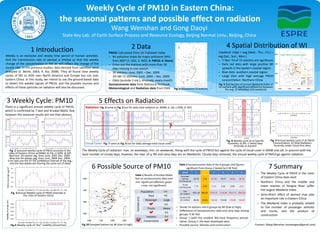
2 Data 4 Spatial Distribution of WI
1 Introduction PM10: Calculated from Air Pollutant Index Weekend Index = avg.(Wed., Thu., Fri.) –
Weekly is an exclusive and steady time period of human activities. High PM10 concentration
– Air pollution index for major pollutant (API) avg.(Sat., Sun., Mon.)
And the transmission rate of aerosol is limited so that the weekly from MEP (1: SO2; 2: NO2; 3. PM10; 4: None) – T-Test: 54 of 72 stations are significant
change of the concentration in the air will reflect the change of the – Cross out the stations with more than 30 – Dark red dots with large positive WI
source rate. In the previous studies, data derived from satellites were days missing in one season spreads in the eastern coastal region
analyzed (S. Beirle, 2003; X. Xia, 2008). They all found clear weekly – 34 stations: June, 2001 – Dec. 2009 – Blue dots: southern coastal region
cycles of NO or AOD over North America and Europe but not over Large WI
34+38=72 stations: June, 2004 – Dec. 2009 – Large dots with high average PM10
Eastern China. In this study, we intend to use the ground-based data – Odds (outside 3 std.); Anomaly: every month concentration: Northern China
to detect the weekly signals of PM10; and the possible sources and Socioeconomic data from Statistical Yearbook Fig. 5 Distribution of annual Weekend Index of
effects of these particles on radiation will also be discussed. 54 stations with significant difference between
Meteorological and Radiation data from CMA Fig. 1 Distribution of stations the avg. of weekdays and weekends
3 Weekly Cycle: PM10 5 Effects on Radiation
a)
a)
There is a significant annual weekly cycle of PM10, Radiation: Fig. 6 same as Fig. 2 but for daily total radiation (a: MAM; b: JJA; c:SON; d: DJF)
which is confirmed by T-test and Kruskal-Wallis Test; b)
however the seasonal results are not that obvious.
?
b)
Fig. 8 Weekly cycle of a) Specific Fig. 9 Annual weekly cycle of a) PM10
Cloud Cover: Fig. 7 same as Fig. 6 but for daily average total cloud cover Humidity; b) RH; c) Rainy Days Concentration; b) Total Radiation
Anomaly in autumn Anomaly under cloud-free skies
Fig. 2 Seasonal weekly cycle of PM10 anomaly in the The Weekly Cycle of radiation: max. on weekdays; min. on weekends. Along with the cycle of PM10 but against the cycle of cloud cover in MAM and JJA. In autumn with the
cities of Eastern China: a) MAM; b) JJA; c) SON; d) DJF. least number of cloudy days, however, the max. of q, RH and rainy days are on Weekends. Cloudy days removed, the annual weekly cycle of PM10 go against radiation.
(Red line: 34-station avg. from June, 2001-Dec. 2009 ;
Blue line:54-station avg. from June, 2004-Dec. 2009;
Error bars are the 97.5% confidence interval of the avg.;
6 Possible Source of PM10 7 Summary
and the two weeks are sharing the same set of data) Table 2 Socioeconomic data of the 6 groups (red figures:
significant from Group 2 tested by K-W Test)
Group 1 2 3 4 5 6
– The Weekly Cycle of PM10 in the cities
Table 1 Results of Kruskal-Wallis Passenger
Test on socioeconomic data (red Vehicles 22.70 7.54 57.95 15.77 29.92 28.33
of Eastern China does exist
Red: 34-station avg., 2002-2009
tick: significant different; green (10 thousand) – Northern China and the middle and
Blue: 72-station avg., 2005-2009
cross: not significant) Trucks
7.13 3.49 9.19 4.24 6.83 8.23 lower reaches of Yangtze River suffer
(10 thousand)
the largest Weekend Index
Fig. 3 Annual Weekly cycle of PM10 anomaly in Population GDP
1651.42 652.61 2378.31 1745.86 2914.72 2603.28
the cities of Eastern China Total
(0.1 billion) – Semi-direct effect of aerosol may play
Construction
an important role in Eastern China
Civil Vehicles
Passenger Large (0.1 billion) 60.35 45.02 132.80 110.60 176.08 152.65
Red: 34-station avg., 2002-2009
Blue: 54-station avg., 2005-2009 – The Weekend Index is probably related
Trucks Heavy – Divide 54 stations into 6 groups by WI (low to high) to the number of passenger vehicles
– Differences of Socioeconomic data and rainy days among and trucks, and the product of
groups: K-W Test construction
Industry – Group 1 (with the smallest WI):most frequency precipi-
GDP
Construction tation; Group 2: the least developed area.
Fig.4 Weekly cycle of “dry” visibility (cloud-free) Fig.10 Grouped stations by WI (low to high) – Possible source: Vehicles and construction Contact: Wang Wenshan (mswangws@gmail.com)