Speaker: Kees de Graaf Date: 22-01-2016 Abstract: We studied the applicability of Credit Valuation Adjustment (CVA) and ANOVA-based dimension reduction in the context of a portfolio of risk factors. Typically, to solve a PDE for multiple risk factors, one has to deal with the curse of dimensionality. Between these risk factors, the correlation is often high, and therefore PCA and ANOVA are promising techniques for dimension reduction and can enable us to compute the exposure profiles for higher dimensional portfolios. In our results, our method is able to compute Exposures (EE, EPE and ENE) and Quantiles for a 10 dimensional problem. That is, a portfolio of three Cross-Currency Swaps, where three different FX rates are modelled with stochastic volatility and stochastic foreign and domestic interest rates. The method is accurate when compared to a full-scale Monte Carlo solution.

1. Efficient CVA computation by risk factor decomposition
Kees de Graaf, Drona Kandhai & Christoph Reisinger
CSL Colloquium Amsterdam, January 2016
de Graaf (2016) Efficient CVA December 2015 1 / 33

2. 1 Credit Valuation Adjustment (CVA) and Counterparty Credit Risk
(CCR)
2 High dimensional problems
3 The forward Kolmogorov PDE
4 Dimension reduction
5 Results
de Graaf (2016) Efficient CVA December 2015 2 / 33

3. Example - I
Suppose you bet with a friend on a Monday in Amsterdam on a day in
October
You will get 100 euro from your friend if :
it rains every single day of the comming week
You’re friend gets 100 euro from you if:
it it is dry for at least one day of the comming week
After one week you exchange the money
de Graaf (2016) Efficient CVA December 2015 3 / 33

4. Example - II
Suppose it rained every day, but:
Your friend gets his bank account hacked with all the money gone;
Your friend spends all his money during the week;
Your friend disappears to Ibiza...
Whom should you charge for the earned, but lost 100 euro? Too late to
think about it after it happened.
de Graaf (2016) Efficient CVA December 2015 4 / 33

5. Intuition of Counterparty Credit Risk (CCR)
CCR analyses risks arising not from the choice of what and where to
gamble, but with whom.
Exposure measures the money at risk depending on what you
gamble.
Credit Value Adjustment (CVA) is a price you charge (or pay) in
order to insure against a possible counterparty default.
Quantiles present worst/best case scenarios.
de Graaf (2016) Efficient CVA December 2015 5 / 33

6. CVA definition
According to Basel III:
Credit Value Adjustment (CVA) ”is the difference between the
risk-free portfolio value and the true portfolio value that takes into
account the possibility of a counterparty’s default”
de Graaf (2016) Efficient CVA December 2015 6 / 33

7. CVA Formula
Mathematically:
CVA(t, T) = (1 − δ)
T
t
EQ
[PE(s)|τ = s] dPD(s) (1)
In practice:
CVA(t, T) ≈ (1 − δ)
N
k=1
q(tk−1, tk)EPE(tk) (2)
PE(t) = Positive Exposure
Q = Risk neutral measure
δ = recovery rate
τ = default time
EPE(t) = (discounted) Expected Positive Exposure
PD(t) = probability density of default before t
q(tk−1, tk) = default prob. in (tk−1, tk)
de Graaf (2016) Efficient CVA December 2015 7 / 33

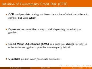
8. Recovery Rate and default probability
Two important ingredients of CVA:
I. Recovery rate δ:
In practice can be deduced from CDS
Taken constant
II. Probability of default PD(t):
Needed at every time t ∈ [t0, T]
Can be modeled or also taken from CDS quotes
de Graaf (2016) Efficient CVA December 2015 8 / 33

9. Exposure
We will focus on the main ingredient of CVA:
III. Expected Positive Exposure EPE(t):
Positive (discounted) future value
Can be computed with Monte Carlo or Forward Kolmogorov PDE
Note that there can be a correlation between default probability and
exposure (Wrong Way Risk)
(A lot of rain ⇐⇒ friend in Ibiza)
de Graaf (2016) Efficient CVA December 2015 9 / 33

10. Earlier related work
Computing Exposure:
[Ng and Peterson (2009)] and [Ng et al. (2010)]: Longstaff-Schwarz
technique compared to FD and nested MC
[de Graaf et al. (2015)]: FDMC for Exposure of portfolios and
sensitivities
[Simaitis et al. (2015)]: Impact of stochastic volatility and rates in CCR
Dimension reduction:
[Reisinger and Wissman (2015a)] and
[Reisinger and Wissman (2015b)]: Methodology and accuracy of lower
dimensional approximations of high-dimensional PDEs
de Graaf (2016) Efficient CVA December 2015 10 / 33

11. High dimensionality
CVA is especially important for portfolios
Due to correlation, risk factors cannot be modeled independently
Finite Difference method cannot handle dimensions greater than 4
(curse of dimensionality)
That is why Monte Carlo is industry standard (scalable)
de Graaf (2016) Efficient CVA December 2015 11 / 33

12. Disadvantages of Monte Carlo
Can also be computationally heavy
Can be problematic for fat tails (Heston and the Feller condition)
Simulation based (non-deterministic)
Can be problematic in the tails of the distribution
de Graaf (2016) Efficient CVA December 2015 12 / 33

13. Challenge
Compute risk measures for a portfolio of FX derivatives assuming many
risk factors, based on real data.
a. FX derivatives:
Typically traded in portfolios
Cross Currency Swaps
b. many risk factors:
Multiple currencies
Smile
Stochastic interest rates
c. real data:
Calibrated models
de Graaf (2016) Efficient CVA December 2015 13 / 33

14. Model Choices
With many risk factors we mean, extend the Black-Scholes model to
include:
a. Stochastic Volatility:
Skew and Smile in FX market
Models: Heston, SABR
b. Stochastic rates:
Vital for long dated derivatives
Hull-White model includes the term structure
Note that this leads to high dimensional models
de Graaf (2016) Efficient CVA December 2015 14 / 33

15. General underlying dynamics
For just one FX rate St, this comes down to:
H-2HW SDEs:



dSt = (rd
t − rf
t )Stdt +
√
VtStdW 1
t ,
dVt = κ(η − Vt)dt + σ
√
VtdW 2
t ,
drd
t = λd (θd (t) − rd
t )dt + ηd dW 3
t ,
drf
t = λf (θf (t) − rf
t ) + ηf ρ1,4
√
Vt dt + ηf dW 4
t ,
dW i
t dW j
t = ρi,j dt, for i = j ∈ 1, . . . 4
de Graaf (2016) Efficient CVA December 2015 15 / 33

16. Resulting PDE
4 dimensional (Kolmogorov-forward) probability density P of one single FX
rate:
∂P
∂t
−
1
2
∂2
∂s2
s2
vP −
1
2
∂2
∂v2
γ2
vP −
1
2
∂2
∂(rd )2
η2
d P −
1
2
∂2
∂(rf )2
η2
f P
+
∂
∂s
(rd
τ − rf
τ )sP +
∂
∂v
(κ(¯v − v)P) +
∂
∂rd
λd (θd
(T − τ) − rd
τ )P
+
∂
∂rf
λf (θf
(T − τ) − rf
τ − ρS,rf ηf
√
v)P + ρS,v
∂2
∂s∂v
(γsvP)
+ ρS,rd
∂2
∂s∂rd
ηd s
√
vP + ρS,rf
∂2
∂s∂rf
ηf s
√
vP + . . . = 0
for three FX rates this will be a 10-dimensional PDE...
de Graaf (2016) Efficient CVA December 2015 16 / 33

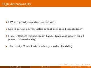
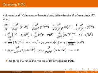
17. Solving the Kolmogorov-Forward PDE
We discretize in every dimension
Partial space derivatives ⇒ finite differences
Use Alternating Direction Implicit scheme for time stepping (see
[in ’t Hout and Foulon(2010)] )
Adjusted for the forward Kolmogorov (see [Itkin. (2015)] )
de Graaf (2016) Efficient CVA December 2015 17 / 33

18. Combining density and payoff
In one plot the procedure is summarized as follows:
0 100 200 300 400 500 600
25
30
35
40
45
50
Vt
time
t = t0 t = tm
at every (Xm
i ),
calculate
V (Xm
i ,tm)
and compute EE as:
N
i=1 P(Xm
i ,tm)V (Xm
i ,tm)
Density
on a grid
t = T
de Graaf (2016) Efficient CVA December 2015 18 / 33

19. Portfolio of Cross Currency Swaps
We are looking at fixed notional floating vs floating cross currency
basis swaps
Notional is exchanged at inception and maturity
The swaps are traded ATM (all cash flows are converted in domestic
currency by the spot FX rate)
EPE is given by:
EPE(t) = max (0, VEURUSD(t) + VEURGBP(t) + VEURJPY(t))
de Graaf (2016) Efficient CVA December 2015 19 / 33

20. Dimension Reduction - I
I. Lower dimensional approximations:
First approximate V assuming only X1
t is stochastic:
V (X1
t ) := V (X1
t , fX1 (t), . . . , fX10 (t)).
where you define fXi s.t.:
fXi (t) = E Xi
t |Xi
t0
= Xi
0
then, compute the higher dimensional approximations:
V (X1
t , X2
t ) :=V (X1
t , X2
t , fX3 (t), . . . , fX10 (t)),
V (X1
t , X3
t ) :=V (X1
t , fX2 (t), X3
t , . . . , fX10 (t)),
...
V (X1
t , X10
t ) :=V (X1
t , fX2 (t), . . . , fX9 (t), X10
t ).
de Graaf (2016) Efficient CVA December 2015 20 / 33

21. Dimension Reduction - II
II. Truncating:
For CCY: we choose only the FX rates as a base
For three dimensions, for example:
V (X1
t , X2
t , X3
t ) = V (X1
t ) + (V (X1
t , X2
t ) − V (X1
t ))
+ (V (X1
t , X3
t ) − V (X1
t ))
+ V (X1
t , X2
t , X3
t ) − V (X1
t , X2
t )
− V (X1
t , X3
t ) − V (X1
t )
We hope that the red part is not so big...
In higher dimensions, corrections will also be higher dimensional
de Graaf (2016) Efficient CVA December 2015 21 / 33

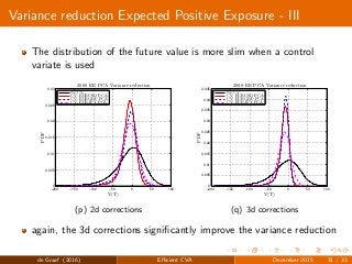
22. Dimension Reduction - III
Definition
Let V (X1
t , . . . , Xn
t ) be the value of a portfolio, driven by n risk factors,
than the k-th 2d ANOVA approximation (where k ∈ [1, . . . , d]) equals:
V k
A(X1
t , . . . , Xn
t ) := V (Xk
t ) + n
i=k V (Xk
t ) − V (Xk
t , Xi
t ) (3)
= (2 − d)V (Xk
t ) + n
i=k V (Xk
t , Xi
t ), (4)
Decomposing the problem
Note that here only one and two-dimensional corrections are needed
We can also use higher order corrections
de Graaf (2016) Efficient CVA December 2015 22 / 33

23. How to find our ”best” ANOVA approximation?
Use the different ANOVA approximations as control variates and
minimize:
min
k∈(1,2,...,n)
Var V k
MC(X1
t , . . . , Xn
t ) , (5)
where V k
MC(X1
t , . . . , Xn
t ) defines the Monte Carlo estimator of
V (X1
t , . . . , Xn
t ) which uses V k
A(X1
t , . . . , Xn
t ) as a control variate
Only a few sample paths are sufficient
de Graaf (2016) Efficient CVA December 2015 23 / 33

24. Market Volatilities
Comparing two used volatility surfaces for EURUSD and EURJPY FX
rate, two completely different markets
0.8 1 1.2 1.4 1.6 1.8 2
9%
10%
11%
12%
13%
14%
15%
2008 EURUSD
Moneyness
Volatility
6M
1Y
2Y
5Y
10Y
(b) Volatility surface in EURUSD.
0.8 1 1.2 1.4 1.6 1.8 2 2.2
8%
10%
12%
14%
16%
18%
20%
22%
2008 EURJPY
Moneyness
Volatility
6M
1Y
2Y
5Y
10Y
(c) Volatility surface in EURJPY.
Smile is inverted (increasing vs decreasing term structure).
Skew is more present in EURJPY.
de Graaf (2016) Efficient CVA December 2015 24 / 33

25. Expected Exposure
Two EE profiles approximated with the help of different PCAs
0 0.5 1 1.5 2 2.5 3 3.5 4 4.5 5
−14
−12
−10
−8
−6
−4
−2
0
2
4
6
2008 PCA: EURUSD
Time
Exposure
u(f1
)
u(f1
,v1
)
u(f1
,f2
)
u(f1
,f3
)
u(f1
,rd
)
u(f1
,rf
)
UPCA (f1
)
UMC (θ)
0 0.5 1 1.5 2 2.5 3 3.5 4 4.5 5
−14
−12
−10
−8
−6
−4
−2
0
2
4
6
2008 PCA: EURJPY
Time
Exposure
u(f3
)
u(f3
,v3
)
u(f3
,f1
)
u(f3
,f2
)
u(f3
,rd
)
u(f3
,rf
)
UPCA (f3
)
UMC (θ)
If we look at relative difference, the EURUSD rate seems to be
slightly more important
Note that the Notional of the EURJPY CCYS is less than the
notional of the EURUSD CCYS
de Graaf (2016) Efficient CVA December 2015 25 / 33

26. Expected Positive Exposure
Two EPE profiles approximated with the help of different PCAs
0 1 2 3 4 5
0
5
10
15
2008 PCA: EURUSD
Time
PositiveExposure
u(f1
)
u(f1
,v1
)
u(f1
,f2
)
u(f1
,f3
)
u(f1
,rd
)
u(f1
,rf
)
UPCA (f1
)
UMC (θ)
0 1 2 3 4 5
0
5
10
15
2008 PCA: EURJPY
Time
PositiveExposure
u(f3
)
u(f3
,v3
)
u(f3
,f1
)
u(f3
,f2
)
u(f3
,rd
)
u(f3
,rf
)
UPCA (f3
)
UMC (θ)
Again the EURUSD rate seems to be more important
de Graaf (2016) Efficient CVA December 2015 26 / 33

27. 3 dimensional corrections - I
If we add three dimensional corrections, results get better
0 0.5 1 1.5 2 2.5 3 3.5 4 4.5 5
−14
−12
−10
−8
−6
−4
−2
0
2
4
6
2008 PCA: EURUSD
Time
Exposure
u(f1
)
u(f1
,v1
)
u(f1
,f2
)
u(f1
,f3
)
u(f1
,rd
)
u(f1
,rf
)
u(f1
,f2
,v2
)
u(f1
,f3
,v3
)
UPCA (f1
)
UMC (θ)
0 0.5 1 1.5 2 2.5 3 3.5 4 4.5 5
−14
−12
−10
−8
−6
−4
−2
0
2
4
6
2008 PCA: EURJPY
Time
Exposure
u(f3
)
u(f3
,v3
)
u(f3
,f1
)
u(f3
,f2
)
u(f3
,rd
)
u(f3
,rf
)
u(f3
,f2
,v2
)
u(f3
,f1
,v1
)
UPCA (f3
)
UMC (θ)
Both EURUSD and EURJPY improve significantly
de Graaf (2016) Efficient CVA December 2015 27 / 33

28. 3 dimensional corrections - II
The same holds for EPE:
0 1 2 3 4 5
0
5
10
15
2008 PCA: EURUSD
Time
PositiveExposure
u(f1
)
u(f1
,v1
)
u(f1
,f2
)
u(f1
,f3
)
u(f1
,rd
)
u(f1
,rf
)
u(f1
,f2
,v2
)
u(f1
,f3
,v3
)
UPCA (f1
)
UMC (θ)
0 1 2 3 4 5
0
5
10
15
2008 PCA: EURJPY
Time
PositiveExposure
u(f3
)
u(f3
,v3
)
u(f3
,f1
)
u(f3
,f2
)
u(f3
,rd
)
u(f3
,rf
)
u(f3
,f2
,v2
)
u(f3
,f1
,v1
)
UPCA (f3
)
UMC (θ)
Downside is that we need to solve 3d PDEs (but we can do that!)
de Graaf (2016) Efficient CVA December 2015 28 / 33

29. Variance reduction Expected Positive Exposure - I
The Variance reduction confirms our findings
0 1 2 3 4 5
0
0.05
0.1
0.15
0.2
0.25
0.3
0.35
0.4
0.45
2008 EE PCA Variance reduction
Time
PCAvar/var
CV: EURUSD PCA
CV: EURGBP PCA
CV: EURJPY PCA
(l) 2d corrections
0 1 2 3 4 5
0
0.05
0.1
0.15
0.2
0.25
0.3
0.35
0.4
0.45
2008 EE PCA Variance reduction
Time
PCAvar/var
CV: EURUSD PCA
CV: EURGBP PCA
CV: EURJPY PCA
(m) 3d corrections
For EE the EURUSD rate is the best PCA
Dimension reduction of around 5 for 2d corrections and almost 100
for 3d corrections
de Graaf (2016) Efficient CVA December 2015 29 / 33

30. Variance reduction Expected Positive Exposure - II
Similar for EPE
0 1 2 3 4 5
0.05
0.1
0.15
0.2
0.25
0.3
0.35
0.4
0.45
0.5
0.55
2008 EPE PCA Variance reduction
Time
PCAvar/var
CV: EURUSD PCA
CV: EURGBP PCA
CV: EURJPY PCA
(n) 2d corrections
0 1 2 3 4 5
0.05
0.1
0.15
0.2
0.25
0.3
0.35
0.4
0.45
0.5
0.55
2008 EPE PCA Variance reduction
Time
PCAvar/var
CV: EURUSD PCA
CV: EURGBP PCA
CV: EURJPY PCA
(o) 3d corrections
The EURUSD rate is the best PCA
Dimension reduction of more than 2 for 2d and around 3 for 3d
corrections
de Graaf (2016) Efficient CVA December 2015 30 / 33

31. Variance reduction Expected Positive Exposure - III
The distribution of the future value is more slim when a control
variate is used
−200 −150 −100 −50 0 50 100
0
0.005
0.01
0.015
0.02
0.025
0.03
2008 EE PCA Variance reduction
V(T)
PDF
No CV
CV: EURUSD PCA
CV: EURGBP PCA
CV: EURJPY PCA
(p) 2d corrections
−200 −150 −100 −50 0 50 100
0
0.005
0.01
0.015
0.02
0.025
0.03
0.035
0.04
0.045
2008 EE PCA Variance reduction
V(T)
PDF
No CV
CV: EURUSD PCA
CV: EURGBP PCA
CV: EURJPY PCA
(q) 3d corrections
again, the 3d corrections significantly improve the variance reduction
de Graaf (2016) Efficient CVA December 2015 31 / 33

32. 2d vs 3d corrections
Pros:
Accuracy improves significant
You can correct for all ”secondary” risk factors (stoch vol and rates)
Variance reductions get slightly better
Cons:
3d PDEs are computationally heavy
Gained variance reduction might not be worth it
de Graaf (2016) Efficient CVA December 2015 32 / 33

33. Summarize
Risk measures:
Many driving risk factors (Portfolios and smile effects)
Tails are difficult (EPE, ENE and quantiles)
Foward Kolmogorov:
Deterministic modeling of the PDF
Dimension reduction:
Approximate high dimensional problems by lower dimensional
approximations
Find the best component by looking at variance reductions of control
variates
Method is extremely scalable (no curse of dimensionality)
de Graaf (2016) Efficient CVA December 2015 33 / 33

34. References I
de Graaf, C. S. L., B. D. Kandhai, and P.M.A. Sloot.
Efficient Estimation of Sensitivities for Counterparty Credit Risk with
the Finite Difference Monte-Carlo Method.
Journal of Computational Finance. Forthcoming.
in ’t Hout, K. J. and S. Foulon.
ADI Finite Difference Schemes For Option Pricing.
International Journal of Numerical Analysis and Modeling 7(2),
303–320.
Ng, L. and D. Peterson.
Potential future exposure calculations using the BGM model.
Wilmott Journal 1(4), 213–225.
de Graaf (2016) Efficient CVA December 2015 34 / 33

35. References II
Ng, L., D. Peterson, and A. E. Rodriguez.
Potential future exposure calculations of multi-asset exotic products
using the stochastic mesh method.
Journal of Computational Finance 14(2).
Itkin, A.
High-Order Splitting Methods for Forward PDEs and PIDEs.
International Journal of Theoretical and Applied Finance, 18(5).
Simaitis, S., C. S. L. de Graaf, N. Hari and B. D. Kandhai.
Smile and Default: The Role of Stochastic Volatility and Interest
Rates in Counterparty Credit Risk.
Submitted, June 2015.
de Graaf (2016) Efficient CVA December 2015 35 / 33

36. References III
Reisinger, C. and R. Wissman.
Numerical Valuation of Derivatives in High-Dimensional Settings via
PDE Expansions.
Journal of Computational Finance, 18(4), 2015.
Reisinger, C. and R. Wissman.
Error Analysis of Truncated Expansion Solutions to High-Dimensional
parabolic PDEs.
Submitted, May 2015.
de Graaf (2016) Efficient CVA December 2015 36 / 33