Inflation theory and analysis Advanced for Msc

1. VII. Inflation
.

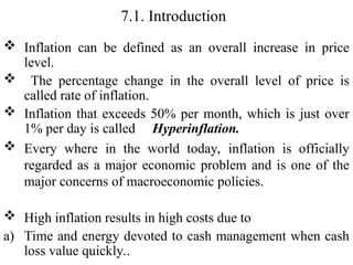
2. 7.1. Introduction
 Inflation can be defined as an overall increase in price
level.
 The percentage change in the overall level of price is
called rate of inflation.
 Inflation that exceeds 50% per month, which is just over
1% per day is called Hyperinflation.
 Every where in the world today, inflation is officially
regarded as a major economic problem and is one of the
major concerns of macroeconomic policies.
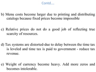
 High inflation results in high costs due to
a) Time and energy devoted to cash management when cash
loss value quickly..

3. Contd….
b) Menu costs become larger due to printing and distributing
catalogs because fixed prices become impossible
c) Relative prices do not do a good job of reflecting true
scarcity of resources.
d) Tax systems are distorted-due to delay between the time tax
is leveled and time tax is paid to government - reduce tax
revenue.
e) Weight of currency become heavy. Add more zeros and
becomes intolerable.

4. 7.2 Excess-Demand or Demand Pull
Inflation
Excess-Demand or Demand Pull Inflation is one of the
earlier theories of inflation.
Inflation is a persistent and appreciable rise in general
level of price.
Inflation is a process of a rising price, not just high
price rise.
That means it is dynamic in nature.

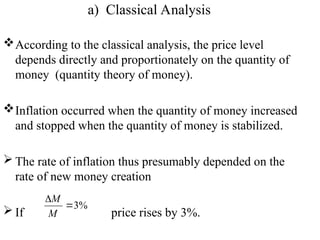
5. a) Classical Analysis
According to the classical analysis, the price level
depends directly and proportionately on the quantity of
money (quantity theory of money).
Inflation occurred when the quantity of money increased
and stopped when the quantity of money is stabilized.
 The rate of inflation thus presumably depended on the
rate of new money creation
 If price rises by 3%.
%
3


M
M

6. If the Economy is at full employment?
New money flowing into the economy in the form of bank
loans to businesses to finance investment in excess of the
current rate of saving leads to net increase in the aggregate
demand for an unchanged total supply of goods (since the
economy was already at full employment).
As a result price of goods increase and also price of inputs
increases, and extract “forced savings” from consumers,
whose money incomes were based on earlier price level.
This leads to monetary inflation which is an excess demand
phenomenon.

7. Ctd
An economy could experience inflation even with a constant
money supply if consumption or investment propensity
increased under condition of full employment.
Full employment:- level of employment beyond which unit
labor cost, and thus price levels, where sure to rise.
If money supplies were constant, higher price would raise
the transaction demand for money and thus push up interest
rates tending to choke off some investment (or consumer)
demand and thus to moderate the inflationary pressure
But it would not completely avoid a rise in price level.

8. Contd….
The reason is that the rise in interest rate would also release
money from idle balance to supply the added transaction
needs at higher price.
Thus same inflation would still occur until interest rate rose
enough to eliminate excess demand.
On the other hand, if government spending increases with
no rise in taxes, the difference (deficit) must be financed
either by:
(a) borrowing from the general public (non-bank) or
borrowing from banks with excess reserve.

9. Ctd…
(b) Printing more paper money,
Condition “b” directly raise price level or
even “a” some times.
Excess of aggregate demand over potential out
put causes prices to bid up until market were
cleared at a price level high enough to
eliminate excess demand.

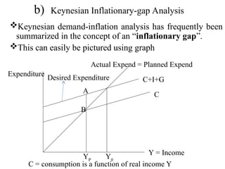
10. b) Keynesian Inflationary-gap Analysis
Keynesian demand-inflation analysis has frequently been
summarized in the concept of an “inflationary gap”.
This can easily be pictured using graph
C
C+I+G
Actual Expend = Planned Expend
Y = Income
Expenditure
A
B
C = consumption is a function of real income Y
YP
Y0
Desired Expenditure

11. Contd….
Assume high level of I + G are independent of the
price level – what ever the price level it will be spent.
The total desired expenditure line = C + I + G
If there was no limit on real output, income would
rise to Y0
, where real expenditure would equal real
output.
But if there is a full employment limit on real output,
Yp, real income can not reach Y0
Yp < Y0

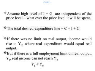
12. Ctd…
At Yp total demand (C + I + G) exceeds total
output, leaving an “inflationary gap” equal to
distance AB
This is the amount by which aggregate
demand at full employment exceeds output at
full employment.
This inflationary gap cause prices to rise.

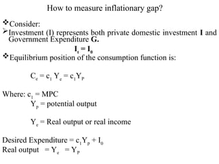
13. How to measure inflationary gap?
Consider:
Investment (I) represents both private domestic investment I and
Government Expenditure G.
It
= I0
Equilibrium position of the consumption function is:
Ce = c1
Ye
= c1
YP
Where: c1
= MPC
Yp = potential output
Ye = Real output or real income
Desired Expenditure = c1
Yp + I0
Real output = Ye = YP

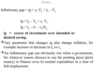
14. Contd….
Inflationary gap = ig = c1 Yp + I0 – Yp
ig = I0
– Yp + c1
Yp
ig = I0
– (1 – c1
)Yp
ig = excess of investment over intended or
desired saving.
Any parameter that changes ig also change inflation, for
example increase or decrease in I0
or c1.
An inflationary gap can obviously rise when a government,
for whatever reason chooses to use the printing press (print
money) to finance even its normal expenditure in a time of
full employment.

15. Contd…..
Inflation from excess demand could also occur during a
strong private investment boom, especially if monetary
policy were willing to “accommodate” increased demands
for money.
Other important causes of excess demand inflation are
usually those associated with war or preparation for war.
When government expenditure typically increases far more
than private expenditures are reduced by higher tax

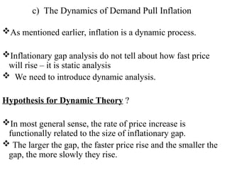
16. c) The Dynamics of Demand Pull Inflation
As mentioned earlier, inflation is a dynamic process.
Inflationary gap analysis do not tell about how fast price
will rise – it is static analysis
 We need to introduce dynamic analysis.
Hypothesis for Dynamic Theory ?
In most general sense, the rate of price increase is
functionally related to the size of inflationary gap.
 The larger the gap, the faster price rise and the smaller the
gap, the more slowly they rise.

17. Contd….
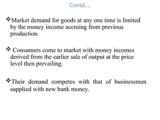
Market demand for goods at any one time is limited
by the money income accruing from previous
production.
 Consumers come to market with money incomes
derived from the earlier sale of output at the price
level then prevailing.
Their demand competes with that of businessmen
supplied with new bank money.

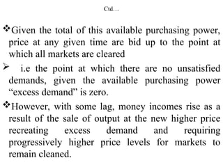
18. Ctd…
Given the total of this available purchasing power,
price at any given time are bid up to the point at
which all markets are cleared
 i.e the point at which there are no unsatisfied
demands, given the available purchasing power
“excess demand” is zero.
However, with some lag, money incomes rise as a
result of the sale of output at the new higher price
recreating excess demand and requiring
progressively higher price levels for markets to
remain cleaned.

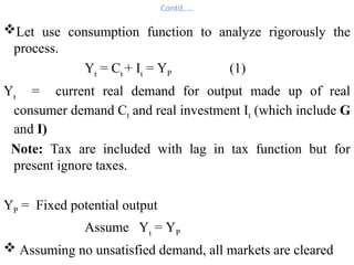
19. Contd…..
Let use consumption function to analyze rigorously the
process.
Yt
= Ct
+ It
= YP (1)
Yt
= current real demand for output made up of real
consumer demand Ct and real investment It (which include G
and I)
Note: Tax are included with lag in tax function but for
present ignore taxes.
YP = Fixed potential output
Assume Yt
= YP
 Assuming no unsatisfied demand, all markets are cleared

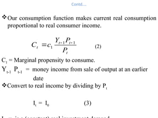
20. Contd….
Our consumption function makes current real consumption
proportional to real consumer income.
t
t
t
t
P
P
Y
c
C 1
1
1


 (2)
C1 = Marginal propensity to consume.
Yt-1
Pt-1
= money income from sale of output at an earlier
date
Convert to real income by dividing by Pt
It = I0 (3)

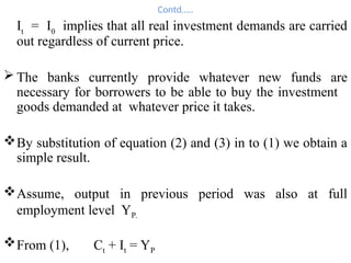
21. Contd…..
It
= I0
implies that all real investment demands are carried
out regardless of current price.
 The banks currently provide whatever new funds are
necessary for borrowers to be able to buy the investment
goods demanded at whatever price it takes.
By substitution of equation (2) and (3) in to (1) we obtain a
simple result.
Assume, output in previous period was also at full
employment level YP.
From (1), Ct + It = YP

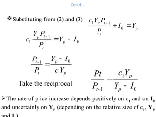
22. Contd….
Substituting from (2) and (3)
p
t
t
p
Y
I
P
P
Y
c



0
1
1
0
1
1 I
Y
P
P
Y
c p
t
t
p



p
p
t
t
Y
c
I
Y
P
P
1
0
1



Take the reciprocal
0
1
1 I
Y
Y
c
P
Pt
p
p
t 


The rate of price increase depends positively on c1
and on I0
and uncertainly on YP
(depending on the relative size of c1
, YP

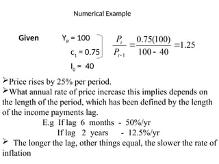
23. Numerical Example
Given YP
= 100
c1
= 0.75
I0
= 40
25
.
1
40
100
)
100
(
75
.
0
1




t
t
P
P
Price rises by 25% per period.
What annual rate of price increase this implies depends on
the length of the period, which has been defined by the length
of the income payments lag.
E.g If lag 6 months - 50%/yr
If lag 2 years - 12.5%/yr
 The longer the lag, other things equal, the slower the rate of
inflation

24. 7.3. Inflation and Phillips Curves
New view of inflation came as a result of the discovery
of empirical regulatory in 1958, by a British Professor
A.W. Phillips.
He studied annual changes in British wage rate over a
period of almost 100 yrs.
Over the first 52 ending 1913 he found fairly stable
relationship between the annual % change in wage rate in
any year and the average level of unemployment.

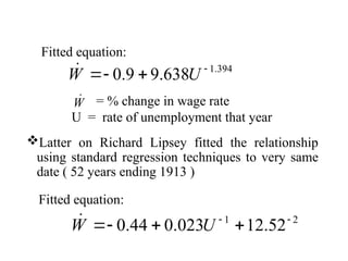
25. Fitted equation:
Latter on Richard Lipsey fitted the relationship
using standard regression techniques to very same
date ( 52 years ending 1913 )
Fitted equation:
2
1
52
.
12
023
.
0
44
.
0 




 U
W

394
.
1
638
.
9
9
.
0 


 U
W

= % change in wage rate
U = rate of unemployment that year
W


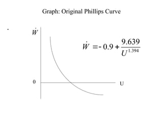
26. A- The Original Phillips Curve
The Original Phillips Curve was an empirical relationship
between the rate of change of money wage ( ) and the rate
of unemployment (U) in the United Kingdom (UK).
What is found was an inverse relationship between the two
convex to the origin which appeared to be remarkably stable
W


27. Ctd…
 Phillips estimated the relationship on the data
from 1861-1913 also found that the
relationship for periods 1913 – 48 and 1948-
57 remained very close to the relationship on
earlier data.
For particular years where the combination
was well away from the estimated curve he
was able to explain in terms of a rise in import
price.

28. Graph: Original Phillips Curve
.
U
0
W

394
.
1
639
.
9
9
.
0
U
W 




29. Contd….
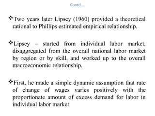
Two years later Lipsey (1960) provided a theoretical
rational to Phillips estimated empirical relationship.
Lipsey – started from individual labor market,
disaggregated from the overall national labor market
by region or by skill, and worked up to the overall
macroeconomic relationship.
First, he made a simple dynamic assumption that rate
of change of wages varies positively with the
proportionate amount of excess demand for labor in
individual labor market

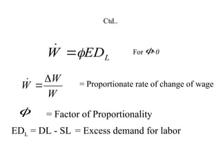
30. Ctd..
L
ED
W 

 For >0
W
W
W


 = Proportionate rate of change of wage
EDL = DL - SL = Excess demand for labor
 = Factor of Proportionality


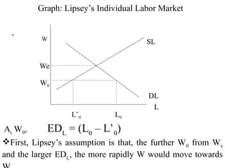
31. Graph: Lipsey’s Individual Labor Market
.
L
W SL
DL
We
W0
L0
L’0
At
W0, EDL
= (L0
– L’0
)
First, Lipsey’s assumption is that, the further W0 from We
and the larger EDL
, the more rapidly W would move towards

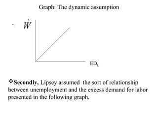
32. Graph: The dynamic assumption
.
EDL
W

Secondly, Lipsey assumed the sort of relationship
between unemployment and the excess demand for labor
presented in the following graph.

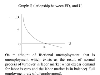
33. Graph: Relationship between EDL and U
.
U
EDL
O
+
- a
Oa = amount of frictional unemployment, that is
unemployment which exists as the result of normal
process of turnover in labor market when excess demand
for labor is zero and the labor market is in balance( Full
employment rate of unemployment).

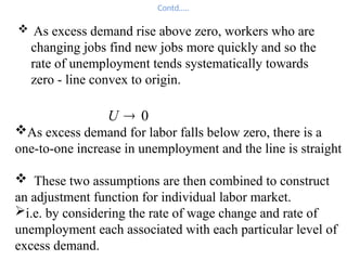
34. Contd…..
 As excess demand rise above zero, workers who are
changing jobs find new jobs more quickly and so the
rate of unemployment tends systematically towards
zero - line convex to origin.
0

U
As excess demand for labor falls below zero, there is a
one-to-one increase in unemployment and the line is straight
 These two assumptions are then combined to construct
an adjustment function for individual labor market.
i.e. by considering the rate of wage change and rate of
unemployment each associated with each particular level of
excess demand.

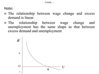
35. Contd….
Note:
o The relationship between wage change and excess
demand is linear.
o The relationship between wage change and
unemployment has the same shape as that between
excess demand and unemployment
W

O
U
a
+
-

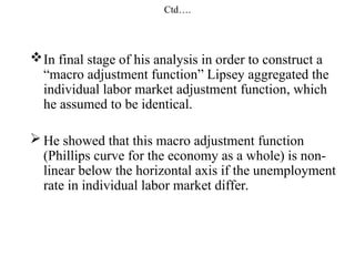
36. Ctd….
In final stage of his analysis in order to construct a
“macro adjustment function” Lipsey aggregated the
individual labor market adjustment function, which
he assumed to be identical.
 He showed that this macro adjustment function
(Phillips curve for the economy as a whole) is non-
linear below the horizontal axis if the unemployment
rate in individual labor market differ.

37. Ctd…
 The further away from the origin the greater is
the difference between unemployment rate in
various individual markets.
The government in principle could shift the
curve towards the origin if it could reduce
dispersion of unemployment rates between
individual labor markets.

38. Contd….
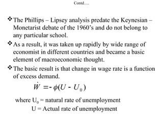
The Phillips – Lipsey analysis predate the Keynesian –
Monetarist debate of the 1960’s and do not belong to
any particular school.
As a result, it was taken up rapidly by wide range of
economist in different countries and became a basic
element of macroeconomic thought.
The basic result is that change in wage rate is a function
of excess demand.
)
( 0
U
U
W 

 

where U0 = natural rate of unemployment
U = Actual rate of unemployment

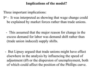
39. Implications of the model?
Three important implications:
1st
- It was interpreted as showing that wage change could
be explained by market forces rather than trade unions.
- This assumed that the major reason for change in the
excess demand for labor was demand shift rather than
(trade union induced) supply shifts.
- But Lipsey argued that trade unions might have effect
elsewhere in the analysis by influencing the speed of
adjustment (Ø) or the dispersion of unemployment, both
of which could affect the position of the Phillips curve.

40. Contd…..
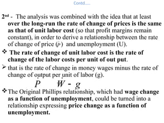
2nd
- The analysis was combined with the idea that at least
over the long-run the rate of change of prices is the same
as that of unit labor cost (so that profit margins remain
constant), in order to derive a relationship between the rate
of change of price ( ) and unemployment (U).
 The rate of change of unit labor cost is the rate of
change of the labor costs per unit of out put.
 that is the rate of change in money wages minus the rate of
change of output per unit of labor (g).
=
The Original Phillips relationship, which had wage change
as a function of unemployment, could be turned into a
relationship expressing price change as a function of
unemployment.
P

P

g
W 


41. Contd……
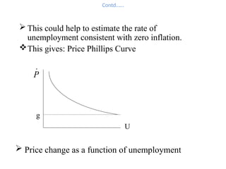
 This could help to estimate the rate of
unemployment consistent with zero inflation.
This gives: Price Phillips Curve
P

U
 Price change as a function of unemployment
g

42. Cntd…..
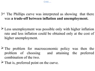
3rd.
The Phillips curve was interpreted as showing that there
was a trade-off between inflation and unemployment.
 Less unemployment was possible only with higher inflation
rate and less inflation could be obtained only at the cost of
higher unemployment.
 The problem for macroeconomic policy was then the
problem of choosing and attaining the preferred
combination of the two.
 That is, preferred point on the curve.

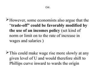
43. Ctd..
However, some economists also argue that the
“trade-off” could be favorably modified by
the use of an incomes policy (set kind of
norm or limit on to the rate of increase in
wages and salaries )
This could make wage rise more slowly at any
given level of U and would therefore shift to
Phillips curve inward to wards the origin

44. 7.4. Expectation-Augmented Phillips Curve
By the Mid 1960 Phillips Curve had been estimated for
variety of countries and time periods with apparent success.
But in late 1960’s and early 1970’s many countries began to
experience combination of inflation and unemployment well
outside the estimated Phillips curve.
 Original Phillips Curve “empirical break down”.
Even before this, however, the original Phillips Curve
analysis had been strongly criticized by Friedman (1968)
and Phelps (1967)
 Critics refer to the figure on excess demand labor of Lipsey
(1960); which shows an upward sloping SL curve and
down ward sloping DL curve drawn against the money
wage on the vertical Axis.

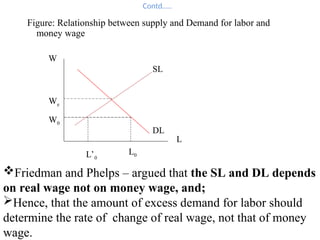
45. Contd…..
Figure: Relationship between supply and Demand for labor and
money wage
L
L0
L’0
W0
We
W
SL
DL
Friedman and Phelps – argued that the SL and DL depends
on real wage not on money wage, and;
Hence, that the amount of excess demand for labor should
determine the rate of change of real wage, not that of money
wage.

46. Contd….
But it is the moneywage which is relevant for the study
of inflation.
The question is then, how does real wage connect to
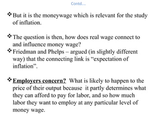
and influence money wage?
Friedman and Phelps – argued (in slightly different
way) that the connecting link is “expectation of
inflation”.
Employers concern? What is likely to happen to the
price of their output because it partly determines what
they can afford to pay for labor, and so how much
labor they want to employ at any particular level of
money wage.

47. Contd…..
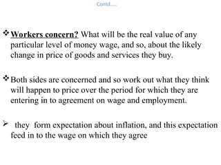
Workers concern? What will be the real value of any
particular level of money wage, and so, about the likely
change in price of goods and services they buy.
Both sides are concerned and so work out what they think
will happen to price over the period for which they are
entering in to agreement on wage and employment.
 they form expectation about inflation, and this expectation
feed in to the wage on which they agree

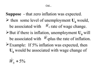
48. Ctd…
Suppose - that zero inflation was expected.
 then some level of unemployment U0
would,
be associated with rate of wage change.
But if there is inflation, unemployment U0
will
be associated with plus the rate of inflation.
Example: If 5% inflation was expected, then
U0
would be associated with wage change of
%
5
0 
W

0
W

0
W


49. Contd…..
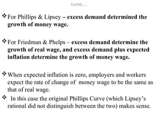
For Phillips & Lipsey – excess demand determined the
growth of money wage.
For Friedman & Phelps – excess demand determine the
growth of real wage, and excess demand plus expected
inflation determine the growth of money wage.
When expected inflation is zero, employers and workers
expect the rate of change of money wage to be the same as
that of real wage.
 In this case the original Phillips Curve (which Lipsey’s
rational did not distinguish between the two) makes sense.

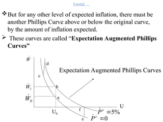
50. Contd…..
But for any other level of expected inflation, there must be
another Phillips Curve above or below the original curve,
by the amount of inflation expected.
 These curves are called “Expectation Augmented Phillips
Curves”
W

0

e
P

%
5

e
P

0
W

1
W

e
f
b
a
c
d
U
U0
Expectation Augmented Phillips Curves

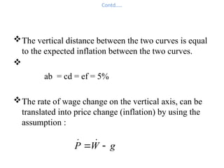
51. Contd…..
The vertical distance between the two curves is equal
to the expected inflation between the two curves.

ab = cd = ef = 5%
The rate of wage change on the vertical axis, can be
translated into price change (inflation) by using the
assumption :
g
W
P 
 


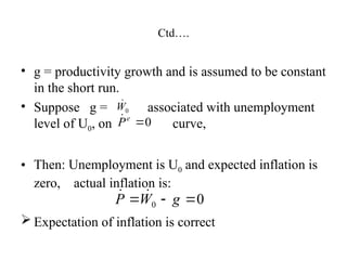
52. Ctd….
• g = productivity growth and is assumed to be constant
in the short run.
• Suppose g = associated with unemployment
level of U0, on curve,
• Then: Unemployment is U0 and expected inflation is
zero, actual inflation is:
 Expectation of inflation is correct
0
W

0

e
P

0
0 

 g
W
P 


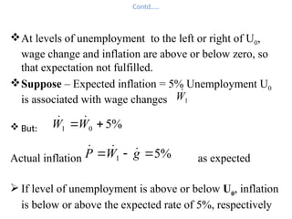
53. Contd…..
At levels of unemployment to the left or right of U0,
wage change and inflation are above or below zero, so
that expectation not fulfilled.
Suppose – Expected inflation = 5% Unemployment U0
is associated with wage changes
 But:
Actual inflation as expected
 If level of unemployment is above or below U0
, inflation
is below or above the expected rate of 5%, respectively
1
W

%
5
0
1 
W
W 

%
5
1 

 g
W
P 



54. Contd…..
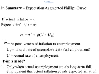
In Summary – Expectation Augmented Phillips Curve
If actual inflation = π
Expected inflation = πe
= responsiveness of inflation to unemployment
U0 = natural rate of unemployment (Full employment)
U = Actual rate of unemployment
Points made?
1. Only when actual unemployment equals long-term full
employment that actual inflation equals expected inflation
)
( 0
U
U
e


 




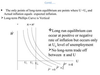
55. Contd……
 The only points of long-term equilibrium are points where U =U0 and
Actual inflation equals expected inflation.
 Long-term Phillips Curve is Vertical
 π = πe
0

e
P
 2

e
P

Long run equilibrium can
occur at positive or negative
rate of inflation but occurs only
at U0
level of unemployment
No long-term trade off
between π and U
4

e
P

U0
U2
U1
W

U

56. Contd……
2. Any attempt to maintain unemployment
permanently below U0
involves a
continuous increase in inflation.
 Conversely any attempt to maintain
unemployment above U0
involves a
continuous decrease in inflation leading
towards zero.

57. 7.5 Adaptive and rational Expectation
 Long-term Phillips Curve which is vertical at the natural
rate of unemployment depends on two things
1) Absence of money illusion, which ensures that expected
inflation is fully incorporated into the determination of
wage change and inflation.
 The difference between different short-run curves must be
equal to the difference between them in expected
inflation.
2) The existence of some mechanism by which actual
inflation is, ultimately if not immediately, fully
incorporated in to expected inflation.
 What is the mechanism?

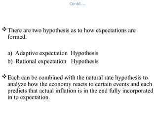
58. Contd…..
There are two hypothesis as to how expectations are
formed.
a) Adaptive expectation Hypothesis
b) Rational expectation Hypothesis
Each can be combined with the natural rate hypothesis to
analyze how the economy reacts to certain events and each
predicts that actual inflation is in the end fully incorporated
in to expectation.

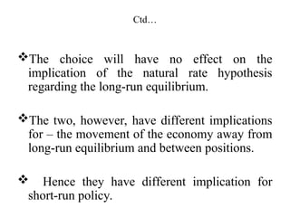
59. Ctd…
The choice will have no effect on the
implication of the natural rate hypothesis
regarding the long-run equilibrium.
The two, however, have different implications
for – the movement of the economy away from
long-run equilibrium and between positions.
 Hence they have different implication for
short-run policy.

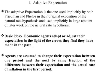
60. 1. Adaptive Expectation
The adaptive Expectation is the one used implicitly by both
Friedman and Phelps in their original exposition of the
natural rate hypothesis and used implicitly in large amount
of later work on the natural rate hypothesis.
Basic idea:- Economic agents adapt or adjust their
expectation in the light of the errors they find they have
made in the past.
Agents are assumed to change their expectation between
one period and the next by same fraction of the
difference between their expectation and the actual rate
of inflation in the first period.

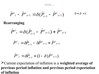
61. Contd……
)
( 1
1
1 

 

 t
e
t
t
e
t
e
P
P
P
P 


 
Rearranging
1
0 


1
1
1 )
( 

 

 t
e
t
e
t
t
e
P
P
P
P 


 
)
)
1
( 1
1 
 

 t
e
t
t
e
P
P
P 

 

1
1
1 

 

 t
e
t
e
t
t
e
P
P
P
P 


 

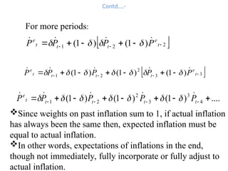
Current expectation of inflation is a weighted average of
previous period inflation and previous period expectation
of inflation

62. Contd….-
 
2
2
1 )
1
(
)
1
( 

 



 t
e
t
t
t
e
P
P
P
P 


 



Since weights on past inflation sum to 1, if actual inflation
has always been the same then, expected inflation must be
equal to actual inflation.
In other words, expectations of inflations in the end,
though not immediately, fully incorporate or fully adjust to
actual inflation.
....
)
1
(
)
1
(
)
1
( 4
3
3
2
2
1 






 


 t
t
t
t
t
e
P
P
P
P
P 



 






 
3
3
2
2
1 )
1
(
)
1
(
)
1
( 


 





 t
e
t
t
t
t
e
P
P
P
P
P 



 






For more periods:

63. Contd….
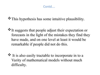
This hypothesis has some intuitive plausibility.
It suggests that people adjust their expectation or
forecasts in the light of the mistakes they find they
have made, and on one level at least it would be
remarkable if people did not do this.
 It is also easily tractable to incorporate in to a
Varity of mathematical models without much
difficulty.

64. Problems with the hypothesis?
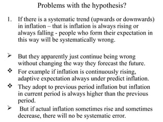
1. If there is a systematic trend (upwards or downwards)
in inflation – that is inflation is always rising or
always falling - people who form their expectation in
this way will be systematically wrong.
 But they apparently just continue being wrong
without changing the way they forecast the future.
 For example if inflation is continuously rising,
adaptive expectation always under predict inflation.
 They adopt to previous period inflation but inflation
in current period is always higher than the previous
period.
 But if actual inflation sometimes rise and sometimes
decrease, there will no be systematic error.

65. Contd…..
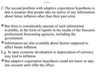
2. The second problem with adaptive expectation hypothesis is
that it assumes that people take no notice of any information
about future inflation other than their past error.
But there is considerable amount of such information
available, in the form of reports in the media of the forecasts
professional forecasting agencies, including the
government.
Information are also available about factors supposed to
affect future inflation.
E.g In open economy devaluation or depreciation of currency
may lead to inflation
But adaptive expectation hypothesis could not know or take
into account until offer the effect.

66. 2. Rational Expectation
Rational Expectation hypothesis in its simplest form
suggests that economic agents use all the information
available to them in trying to forecast the future.
Assumptions:-
a - Economic agents make their forecast as if on the basis of a
current model of the economy, and,
b - This current model includes the systematic element in
government policy.
According to the first assumption, agents understand the
natural rate hypothesis, realize that nominal aggregate
demand is determined by the growth of the money supply,
know the value of U0
and so on

67. Contd…..
The Weak version of the hypothesis argue that, when the
govt. decide to increase the growth of the money supply
from g to g + 5%, people immediately perceive it and
realize that this brings about an inflation rate of 5% and
expect inflation of 5%.
Stronger version of the hypothesis argue that people
understand how the government typically manipulates its
monetary policy.
 Understand that if unemployment rises by j% above U0
the
govt. reacts by increasing monetary growth by k%

68. Ctd…
Therefore, whenever unemployment rises
above U0
by j% people expect the govt. to
increase monetary growth by k%, and
immediately revise their expectation of
inflation accordingly.
Problem: - Cost of acquiring the information
-Finding (choosing) the correct
model of the economy
- Knowing the typical behavior of
the authorities manipulating the policy

69. 7.6. Cost – Push Inflation
Cost – Push Inflation theory was important in the
1960s and 1970s when it formed the key element of
the Keynesian side in the Keynesian – Monetarist
debate and has become less important and prominent
since then
However, it is worth discussing for more than
theoretical reason because some legacy of this idea
persist in mainstream economics in the form of the
possibility of certain kinds of supply side shock.
For easy understanding, think of the price of an
individual good produced by a particular firm.

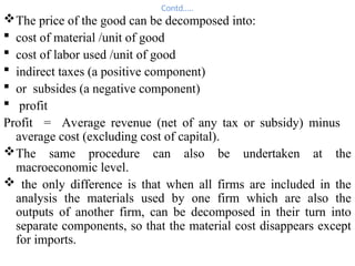
70. Contd…..
The price of the good can be decomposed into:
 cost of material /unit of good
 cost of labor used /unit of good
 indirect taxes (a positive component)
 or subsides (a negative component)
 profit
Profit = Average revenue (net of any tax or subsidy) minus
average cost (excluding cost of capital).
The same procedure can also be undertaken at the
macroeconomic level.
 the only difference is that when all firms are included in the
analysis the materials used by one firm which are also the
outputs of another firm, can be decomposed in their turn into
separate components, so that the material cost disappears except
for imports.

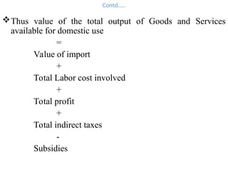
71. Contd…..
Thus value of the total output of Goods and Services
available for domestic use
=
Value of import
+
Total Labor cost involved
+
Total profit
+
Total indirect taxes
-
Subsidies

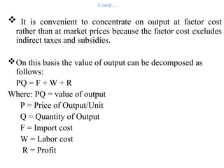
72. Contd….
 It is convenient to concentrate on output at factor cost
rather than at market prices because the factor cost excludes
indirect taxes and subsidies.
On this basis the value of output can be decomposed as
follows:
PQ = F + W + R
Where: PQ = value of output
P = Price of Output/Unit
Q = Quantity of Output
F = Import cost
W = Labor cost
R = Profit

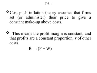
73. Ctd….
Cost push inflation theory assumes that firms
set (or administer) their price to give a
constant make-up above costs.
 This means the profit margin is constant, and
that profits are a constant proportion, r of other
costs.
R = r(F + W)

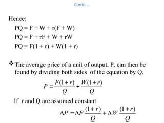
74. Contd….
Hence:
PQ = F + W + r(F + W)
PQ = F + rF + W + rW
PQ = F(1 + r) + W(1 + r)
The average price of a unit of output, P, can then be
found by dividing both sides of the equation by Q.
Q
r
W
Q
r
F
P
)
1
(
)
1
( 



If r and Q are assumed constant
Q
r
W
Q
r
F
P
)
1
(
)
1
( 







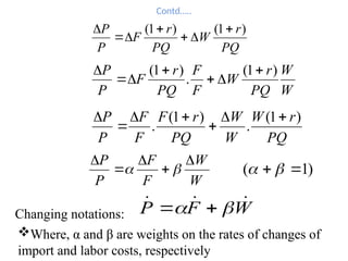
75. Contd…..
PQ
r
W
PQ
r
F
P
P )
1
(
)
1
( 






W
W
PQ
r
W
F
F
PQ
r
F
P
P )
1
(
.
)
1
( 






PQ
r
W
W
W
PQ
r
F
F
F
P
P )
1
(
.
)
1
(
.







W
W
F
F
P
P 





 )
1
( 
 

Where, α and β are weights on the rates of changes of
import and labor costs, respectively
W
F
P 

 
 

Changing notations:

76. Contd…..
With constant profit margin, the change in price is a
function of change in import cost and change in labor cost.
If output at market price was being considered, the change
in indirect taxes and subsidies would figure in the equation.
Cost push inflation theory regards the labor cost change and
import cost change as proximate determinants of inflation.
Particularly change in labor costs are singled out as the
main causes of inflation.
In the 1970s and 1980s, a number of studies tried to relate
the change in labor cost to some measures or indicator of
trade unions militancy.

77. Contd…..
Thus inflation is seen as caused by increase in costs;
variation in demand have no direct effect on prices
and indeed no indirect effect either, since cost push
theories generally consider that the rate of change of
wages is also independent of demand conditions.
Thus the appropriate way to reduce or prevent
inflation is the use of an income policy that reduce
the rate at which wages increase.
Spiral = Wage increases lead to Price increases and this
in turn leads to inflation

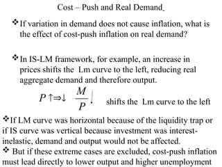
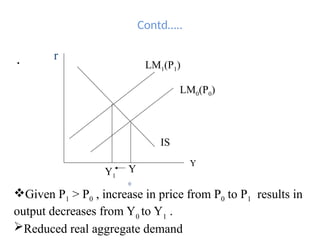
78. Cost – Push and Real Demand
If variation in demand does not cause inflation, what is
the effect of cost-push inflation on real demand?
In IS-LM framework, for example, an increase in
prices shifts the Lm curve to the left, reducing real
aggregate demand and therefore output.
P
M
P  shifts the Lm curve to the left
If LM curve was horizontal because of the liquidity trap or
if IS curve was vertical because investment was interest-
inelastic, demand and output would not be affected.
 But if these extreme cases are excluded, cost-push inflation
must lead directly to lower output and higher unemployment

79. Contd…..
.
Y
r
LM0(P0)
LM1(P1)
Y
0
Y1
Given P1 > P0 , increase in price from P0 to P1 results in
output decreases from Y0
to Y1
.
Reduced real aggregate demand
IS

80. Contd…..
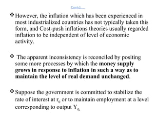
However, the inflation which has been experienced in
most industrialized countries has not typically taken this
form, and Cost-push inflations theories usually regarded
inflation to be independent of level of economic
activity.
 The apparent inconsistency is reconciled by positing
some more processes by which the money supply
grows in response to inflation in such a way as to
maintain the level of real demand unchanged.
Suppose the government is committed to stabilize the
rate of interest at r0
or to maintain employment at a level
corresponding to output Y0.

81. Contd…..
.
LM0(M0,P0)
LM1(M0,P1)
LM2(M1,P1)
Y
r
Y0
Y1
r1
r0
If cost-push pressure increases the price level from P0 to
P1 and the LM curve shifts to the left from LM0 to LM1,
the rate of interest will tend to rise to r1 and the level of
aggregate demand and output to fall to Y1.

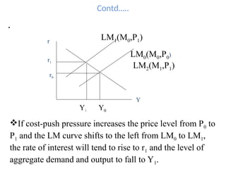
82. Contd…..
However, the government could prevent either or both of
these things occurring by increasing the nominal money
supply from M0 to M1so that the LM curve shifts back to its
original position at LM2.
 Counter balance the tendency of r to increase to r1
and the
tendency of Y to decrease to Y1
by increasing the nominal
money supply.
 Thus the growth of the money supply is caused by and
endogenous to inflation here, in such a way as to eliminate
the effect inflation would otherwise have had on the level of
economic activity.
 The endogeneity also makes sense of the observed tendency
for prices and money to rise together over long time period.

83. Contd…..
 An alternative possibility is that the response of money supply to
inflation may not be only due to any commitment or specific
decisions by the government, but also due to some monetary
control system.
E.g Cost-push inflation might increase budget deficit if it
tends to increase nominal government expenditure by more than it
increases tax revenue.
If not reacted by increasing government borrowing from private
sector money supply will increase.
A second example is where bank lending to the private sector is
determined essentially by demand for credit, cost-push inflation
leads companies to borrow more to maintain the real value of
their working capital.

84. Contd…..
That means, bank lending and the money
supply will increase in line with prices.
The precise mechanism involved has not
been well developed, there is little empirical
analysis.
But some mechanism that makes money
supply endogenous to inflation is essential to
cost-push inflation theory.