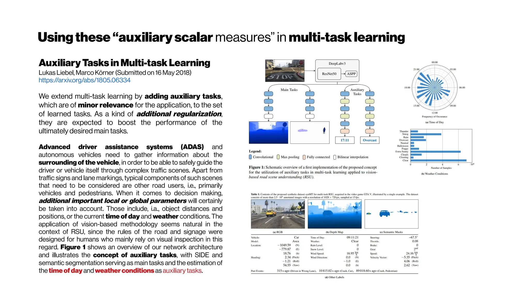
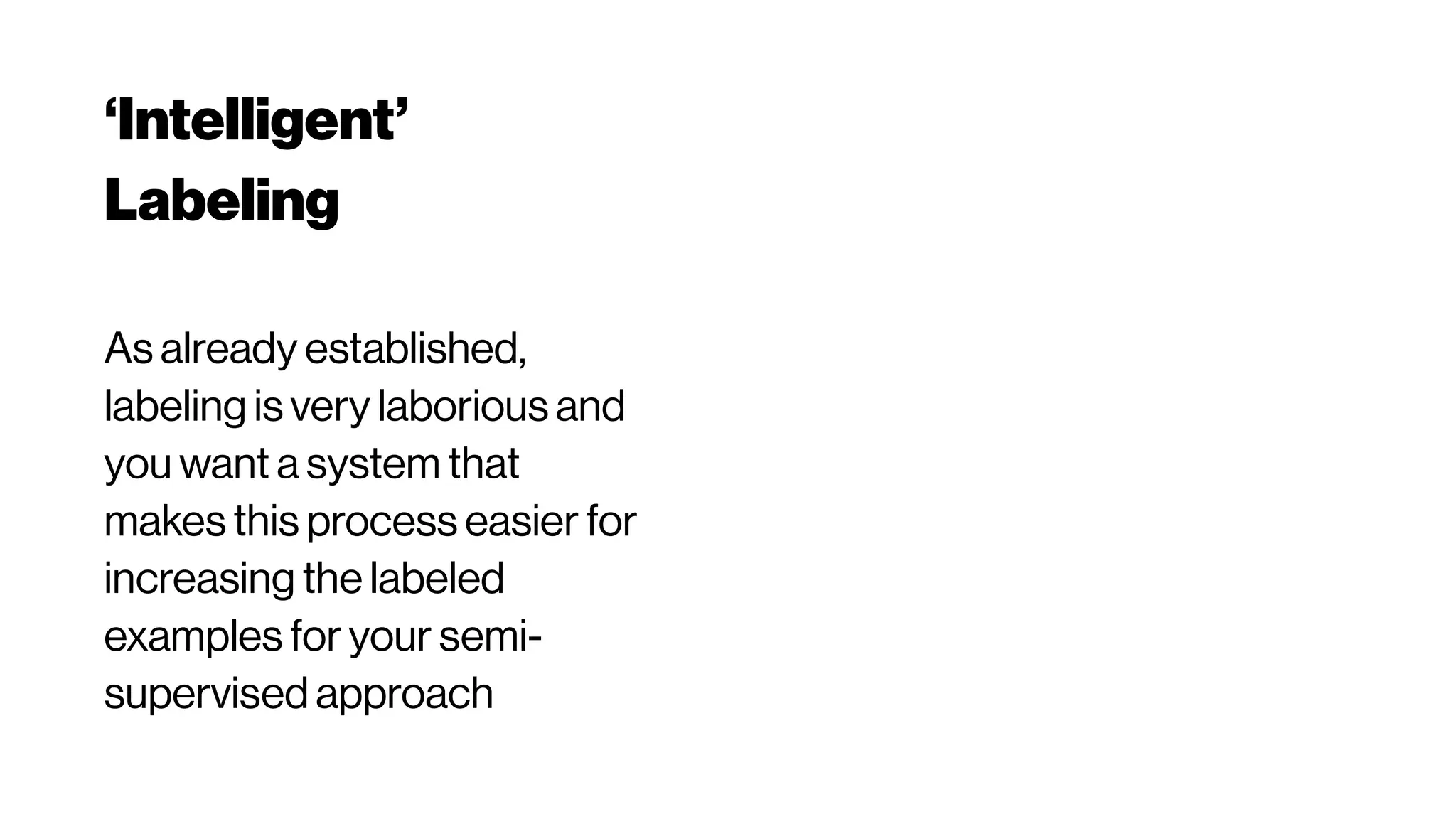
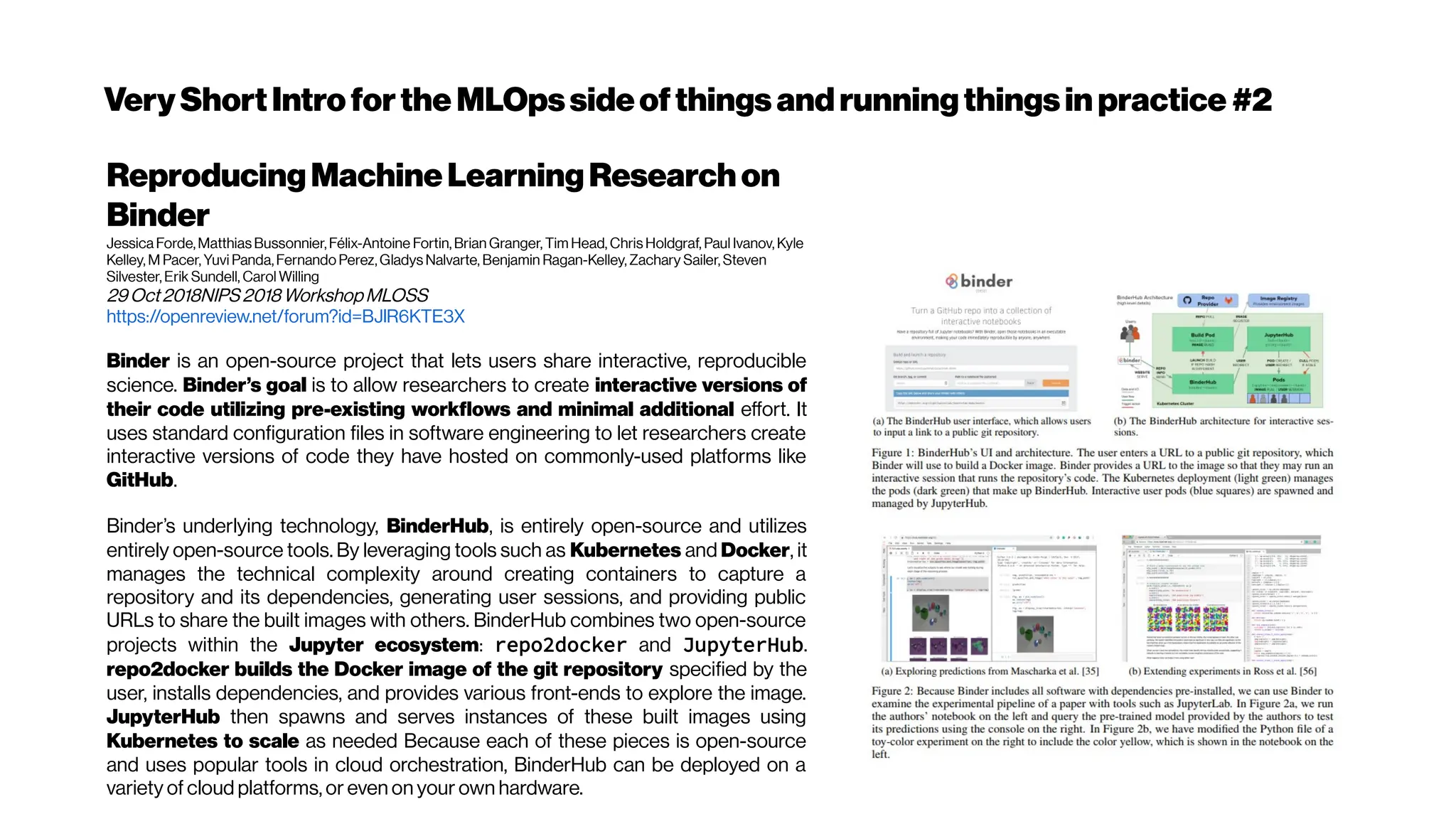
Download as PDF, PPTX


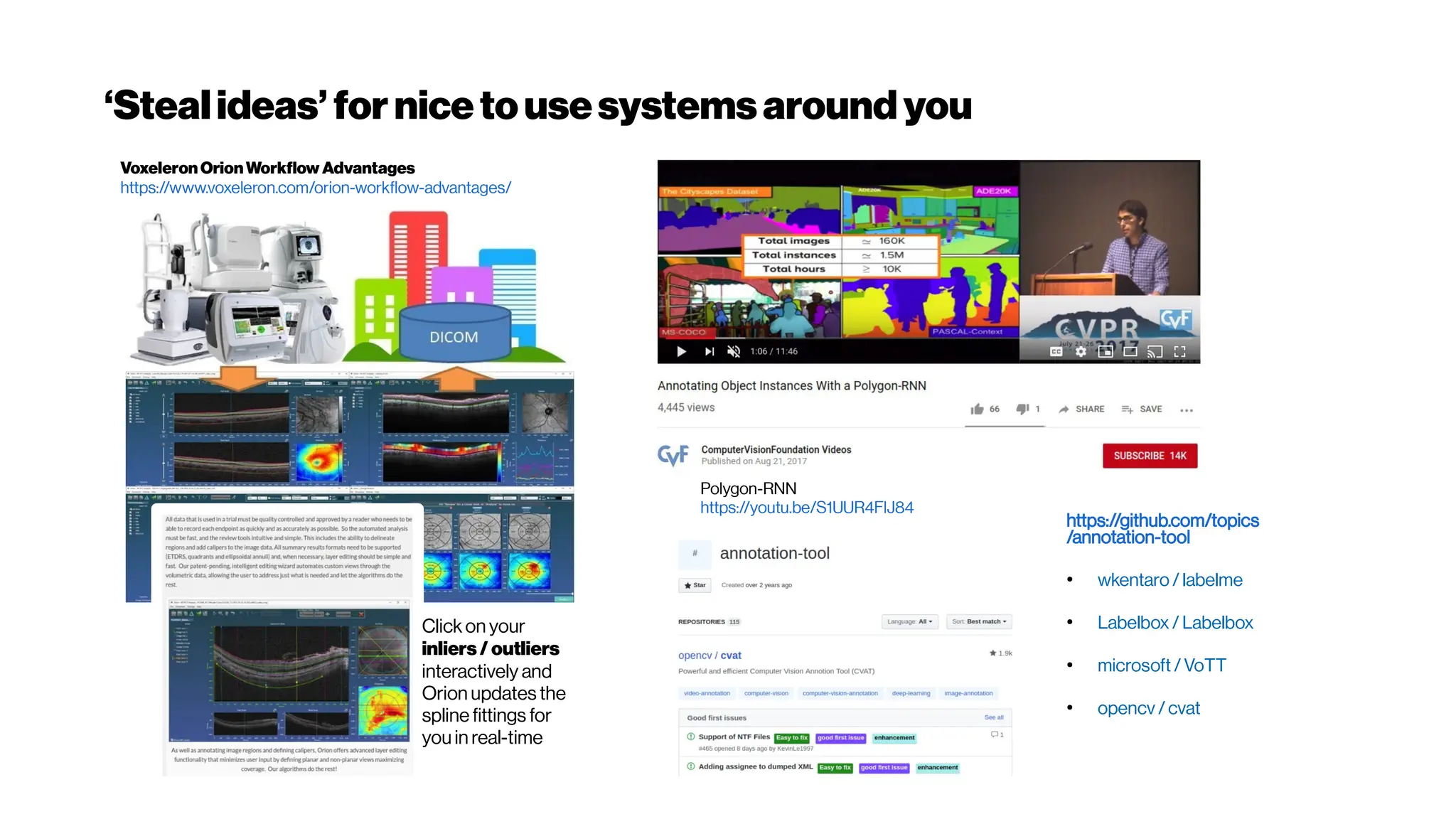
![Voxel Mesh
→ conversion“trivial”withcorrectsegmentation/graph model
DeepMarchingCubes:LearningExplicitSurface
Representations
Yiyi Liao, Simon Donńe, Andreas Geiger (2018)
https://avg.is.tue.mpg.de/research_projects/deep-marching-cubes
http://www.cvlibs.net/publications/Liao2018CVPR.pdf
https://www.youtube.com/watch?v=vhrvl9qOSKM
Moreover, we showed that surface-based supervision results in better
predictions in case the ground truth 3D model is incomplete. In future
work, we plan to adapt our method to higher resolution outputs using
octrees techniques [Häne et al. 2017; Riegler et al. 2017; Tatarchenko et al. 2017]
and integrate
our approach with other input modalities
Learning3DShapeCompletionfromLaserScanDatawithWeakSupervision
David Stutz, Andreas Geiger (2018)
http://openaccess.thecvf.com/content_cvpr_2018/CameraReady/1708.pdf
Deep-learning-assistedVolumeVisualization
Hsueh-Chien Cheng, Antonio Cardone, Somay Jain, Eric Krokos, Kedar Narayan, Sriram Subramaniam,
Amitabh Varshney
IEEE Transactions on Visualization and Computer Graphics ( 2018)
https://doi.org/10.1109/TVCG.2018.2796085
Although modern rendering techniques and hardware can now render volumetric data
interactively, we still need a suitablefeaturespace that facilitates naturaldifferentiationof
target structures andan intuitive and interactive way of designing visualizations](https://image.slidesharecdn.com/multiphotonsegmentation2024-240117012649-7950e327/75/Two-Photon-Microscopy-Vasculature-Segmentation-29-2048.jpg)

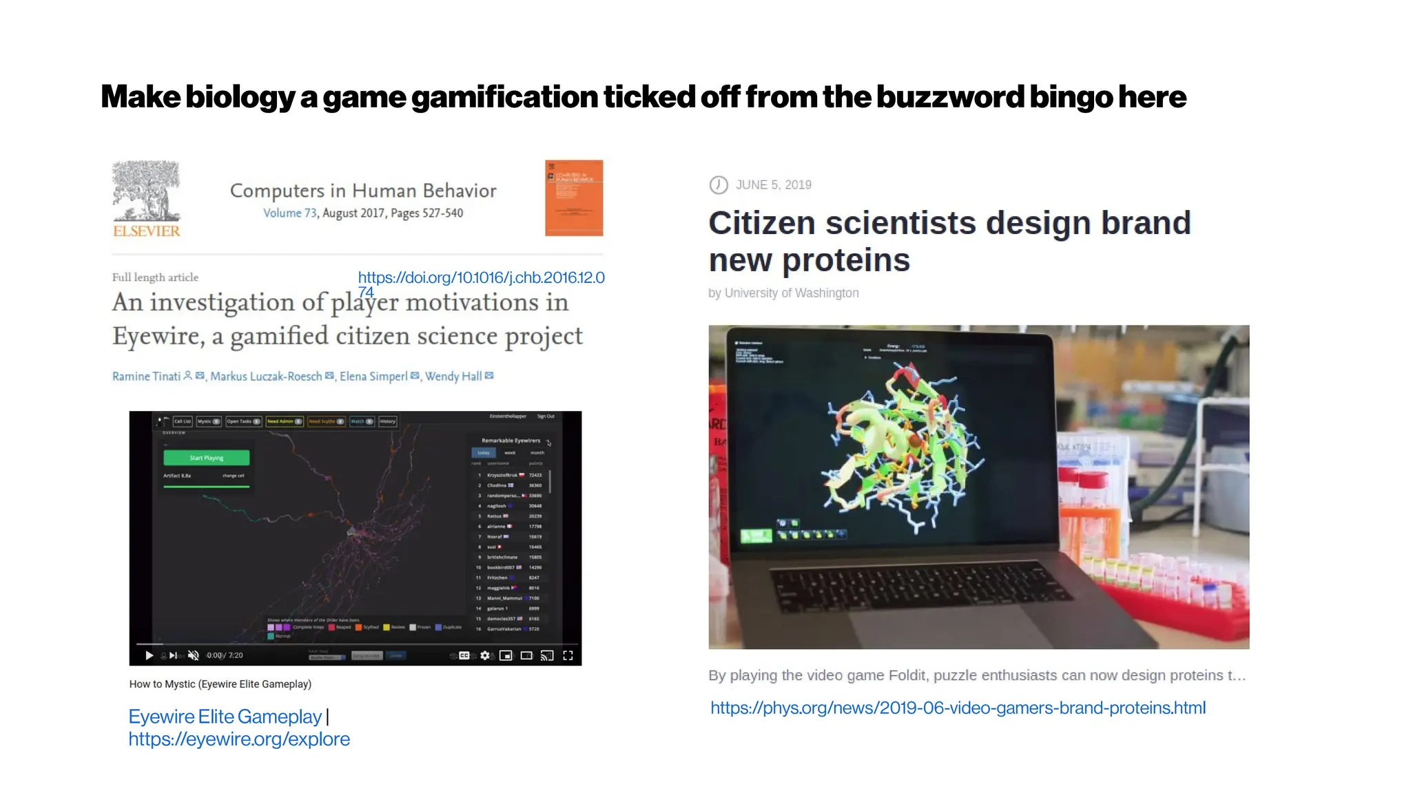
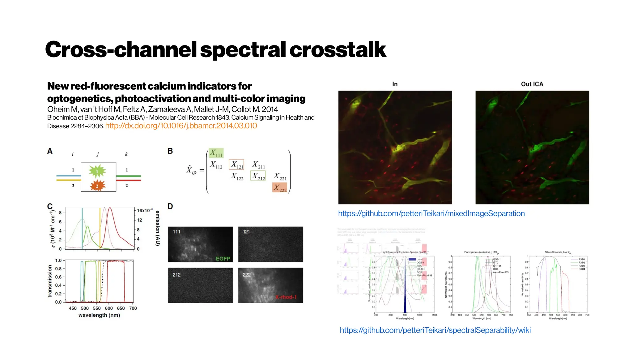
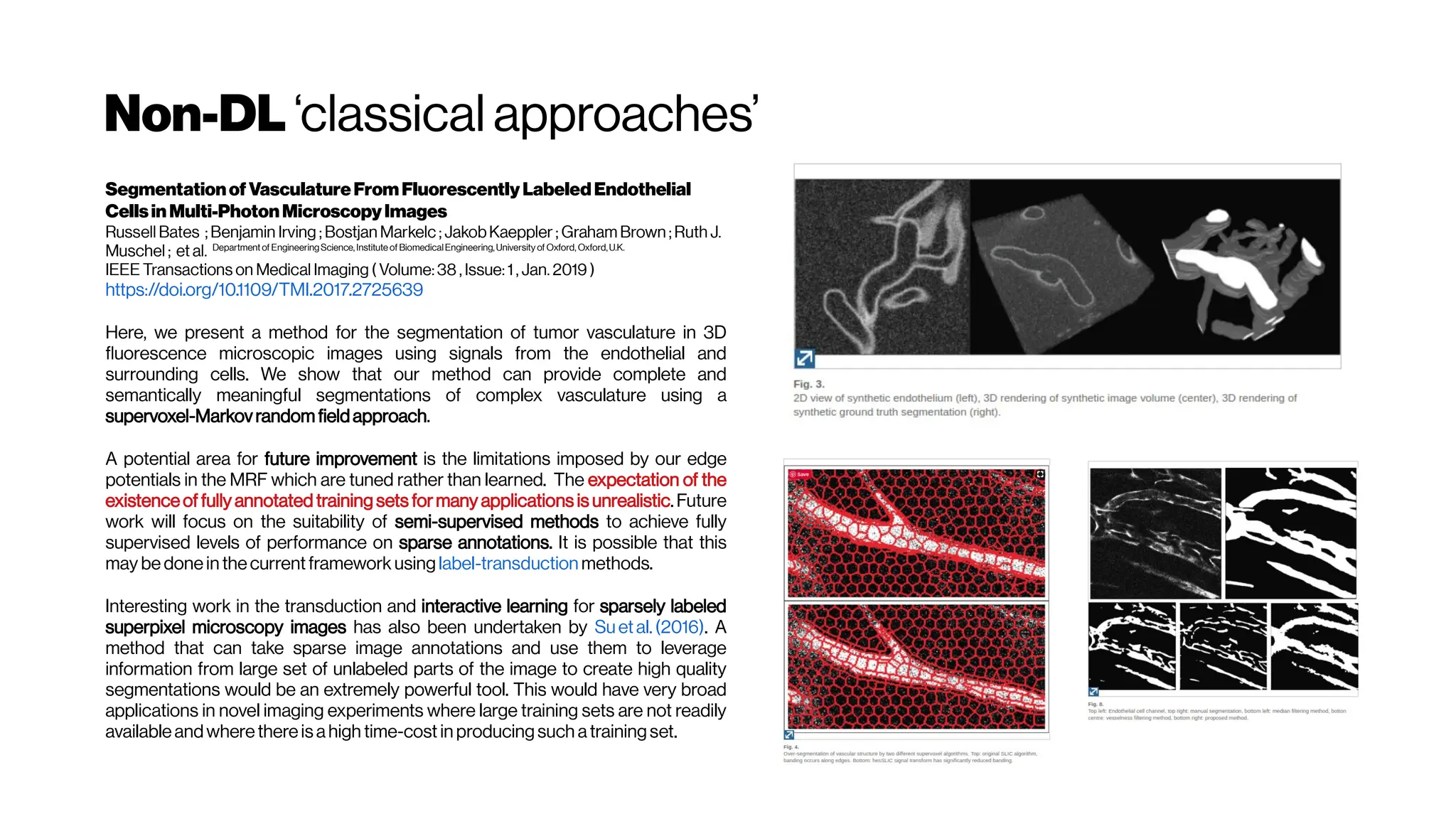
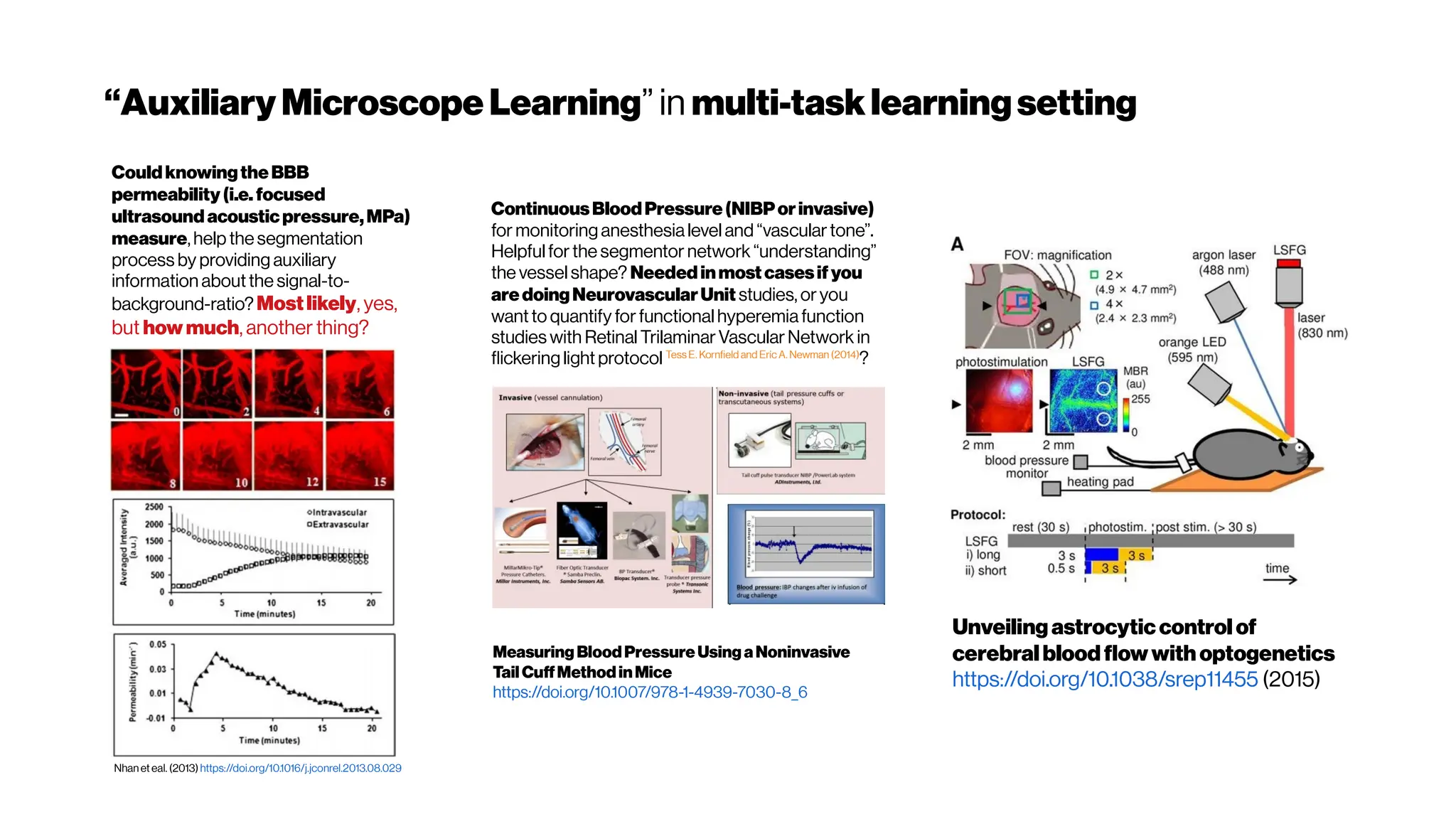
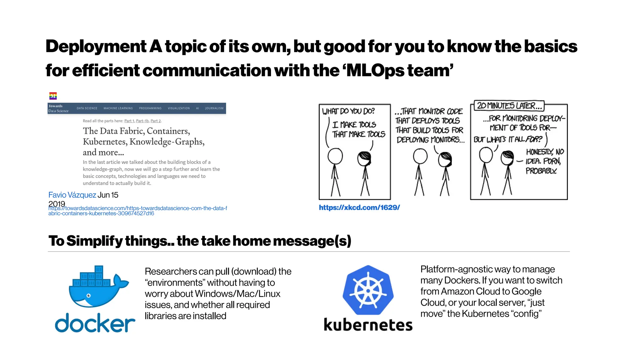
![VasculatureNetworks Multimodali.e.“multidye”
3DCNNsifpossible
HyperDense-Net:A hyper-densely connected
CNN formulti-modal image segmentation
Jose Dolz
https://arxiv.org/abs/1804.02967(9 April 2018)
https://www.github.com/josedolz/HyperDenseNe
t
We propose HyperDenseNet, a 3D fully convolutional
neural network that extends the definition of dense
connectivity to multi-modal segmentation problems
[MRI Modalities: MR-T1, PD MR-T2,
FLAIR]. Each imaging modality has a path, and dense
connections occur not only between the pairs of
layers within the same path, but also between those
across different paths.
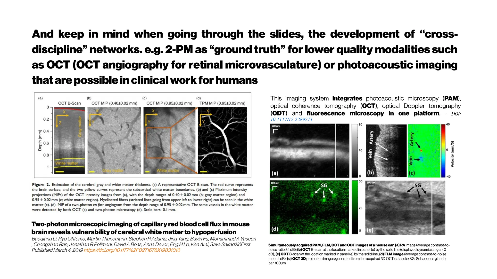
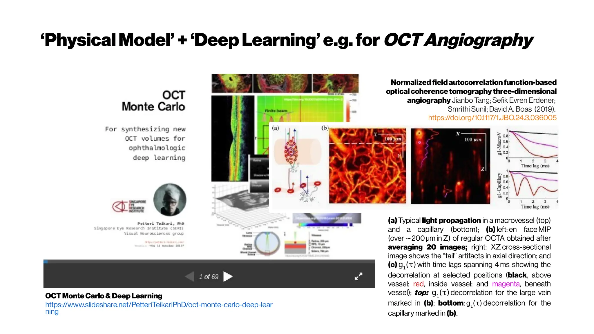
A multimodal imaging platform with integrated
simultaneousphotoacousticmicroscopy, optical
coherencetomography,optical Doppler tomography
and fluorescence microscopy
Arash Dadkhah; Jun Zhou; Nusrat Yeasmin; Shuliang Jiao
https://sci-hub.tw/https://doi.org/10.1117/12.2289211
(2018)
Here, we developed a multimodal optical imaging system with
the capability of providing comprehensive structural,
functional and molecular information of living tissue in
micrometer scale.
An artery-specificfluorescent dye for studying
neurovascularcoupling
Zhiming Shen, Zhongyang Lu, Pratik Y Chhatbar, Philip
O’Herron, and Prakash Kara
https://dx.doi.org/10.1038%2Fnmeth.1857(2012)
Here, we developed a multimodal optical imaging system with
the capability of providing comprehensive structural,
functional and molecular information of living tissue in
micrometer scale.
Astrocytes are intimatelylinked to the function
of the inner retinalvasculature. A flat-mounted
retina labelled for astrocytes (green) and retinal
vasculature (pink). - from Prof Erica Fletcher](https://image.slidesharecdn.com/multiphotonsegmentation2024-240117012649-7950e327/75/Two-Photon-Microscopy-Vasculature-Segmentation-54-2048.jpg)

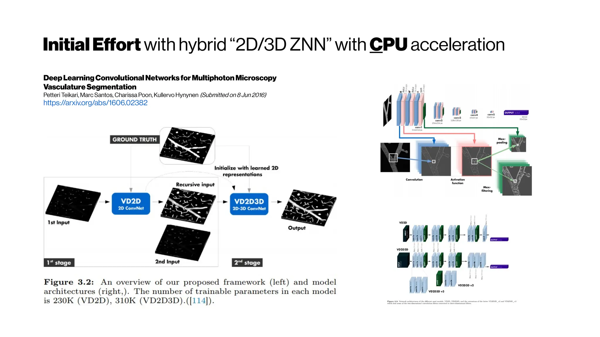
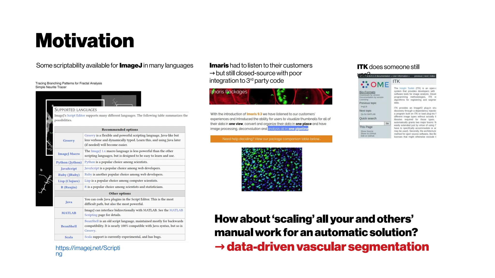
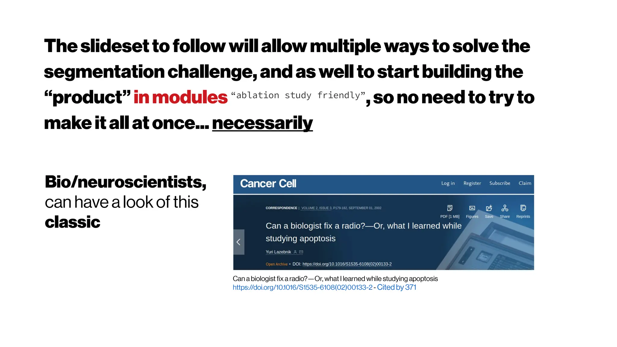
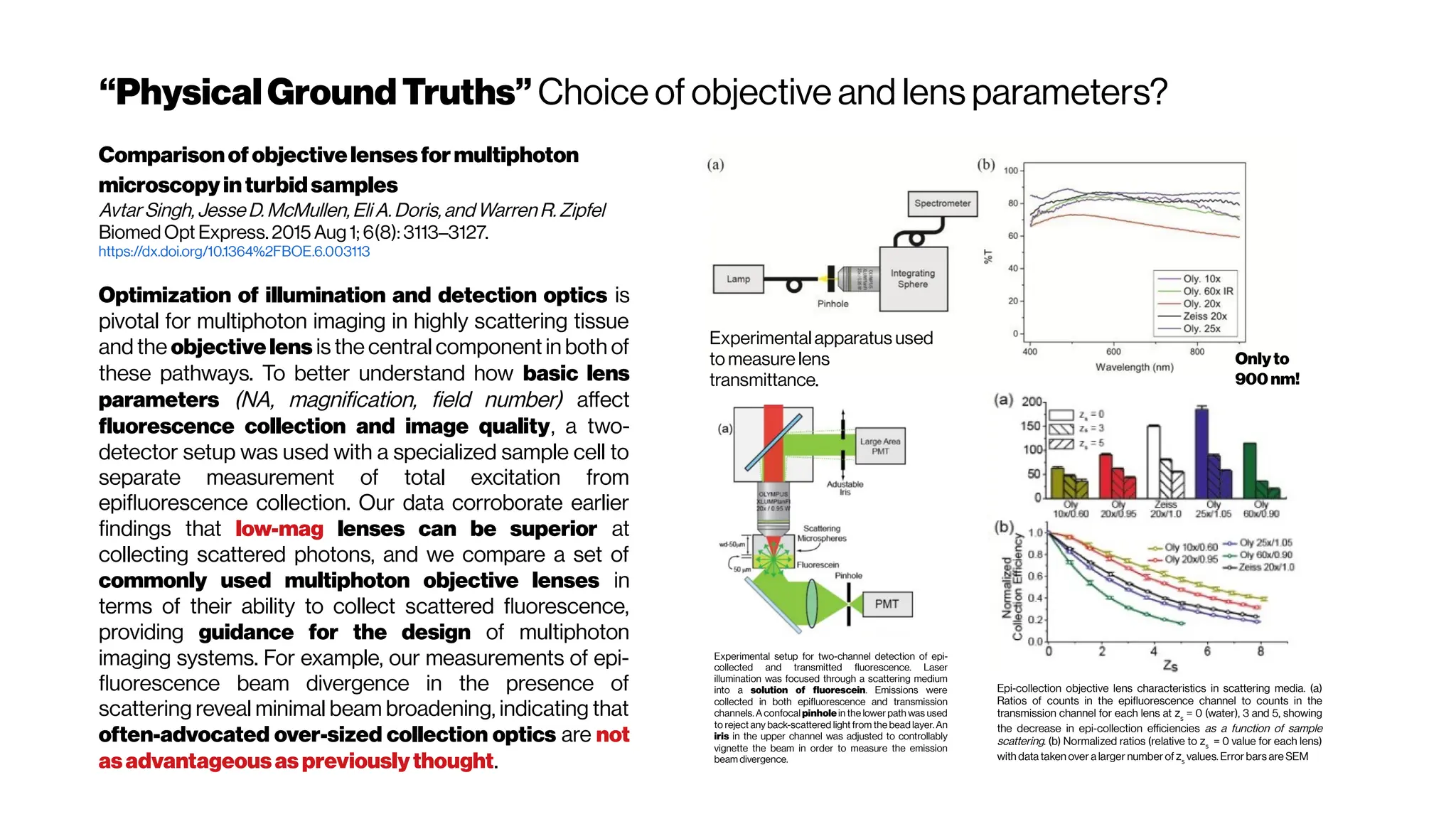
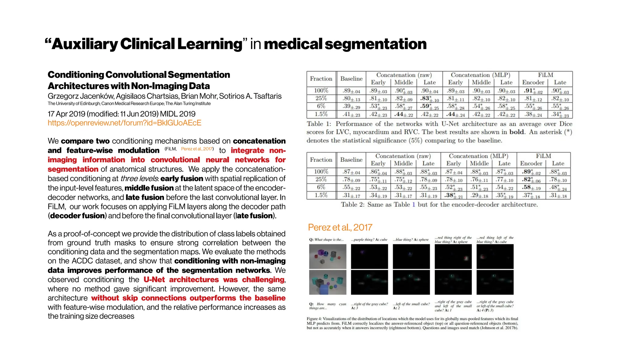
![MicrovasculatureCNNs #5
A Deep Learning Approach to 3D Segmentation of Brain Vasculature
Waleed Tahir, Jiabei Zhu, Sreekanth Kura,Xiaojun Cheng,DavidBoas,
and Lei Tian (2019)
Department of Electrical and Computer Engineering, Boston University
https://www.osapublishing.org/abstract.cfm?uri=BRAIN-2019-BT2A.6
The segmentation of blood-vessels is an important preprocessing
step for the quantitative analysis of brain vasculature. We approach
the segmentation task for two-photon brain angiograms using a fully
convolutional 3D deep neural network.
We employ a DNN to learn a statistical model relating the measured
angiograms to the vessel labels. The overall structure is derived from
V-net [Milletari et al.2016] which consists of a 3D encoder-decoder
architecture. The input first passes through the encoder path which
consists of four convolutional layers. Each layer comprises of residual
connections which speed up convergence, and 3D convolutions with
multi-channel convolution kernels which retain 3D context.
Loss functions like mean squared error (MSE) and mean absolute
error (MAE) have been used widely in deep learning, however, they
cannot promote sparsity and are thus unsuitable for sparse objects. In
our case, less than 5% of the total volume in the angiogram comprises
of blood vessels. Thus, the object under study is not only sparse, there
is also a large class-imbalance between the number for foreground vs.
background voxels. Thus we resort to balanced cross entropy as the
loss function [HED, 2015], which not only promotes sparsity, but also
caters fortheclass imbalance](https://image.slidesharecdn.com/multiphotonsegmentation2024-240117012649-7950e327/75/Two-Photon-Microscopy-Vasculature-Segmentation-101-2048.jpg)
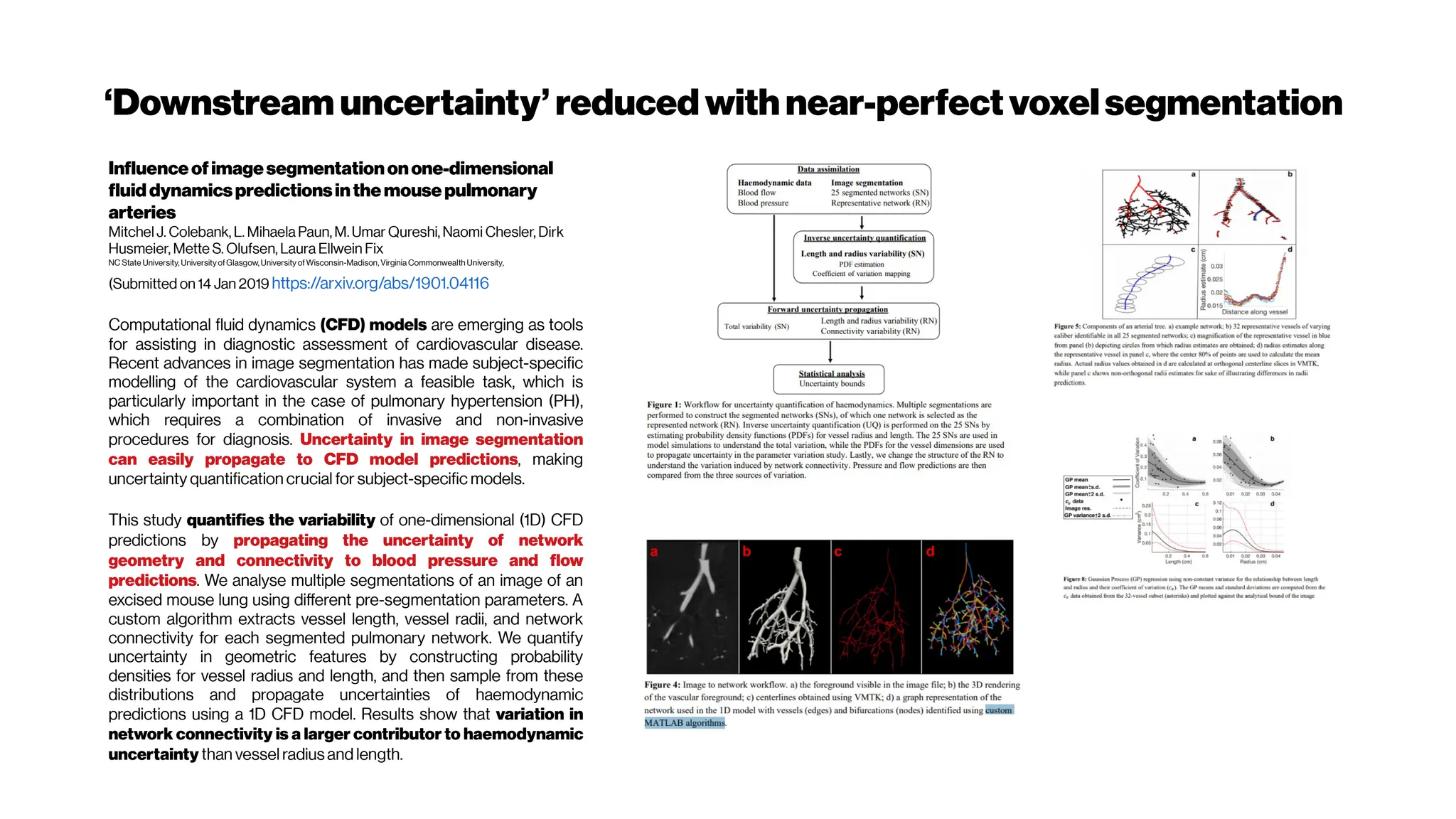
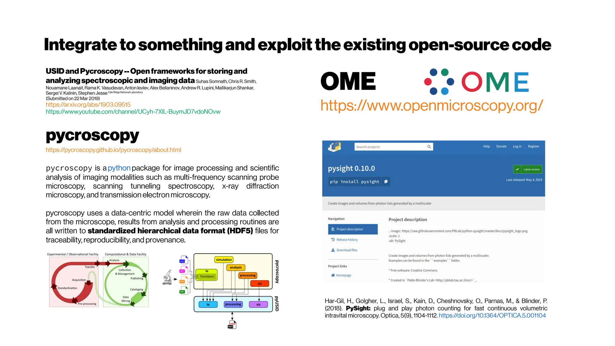
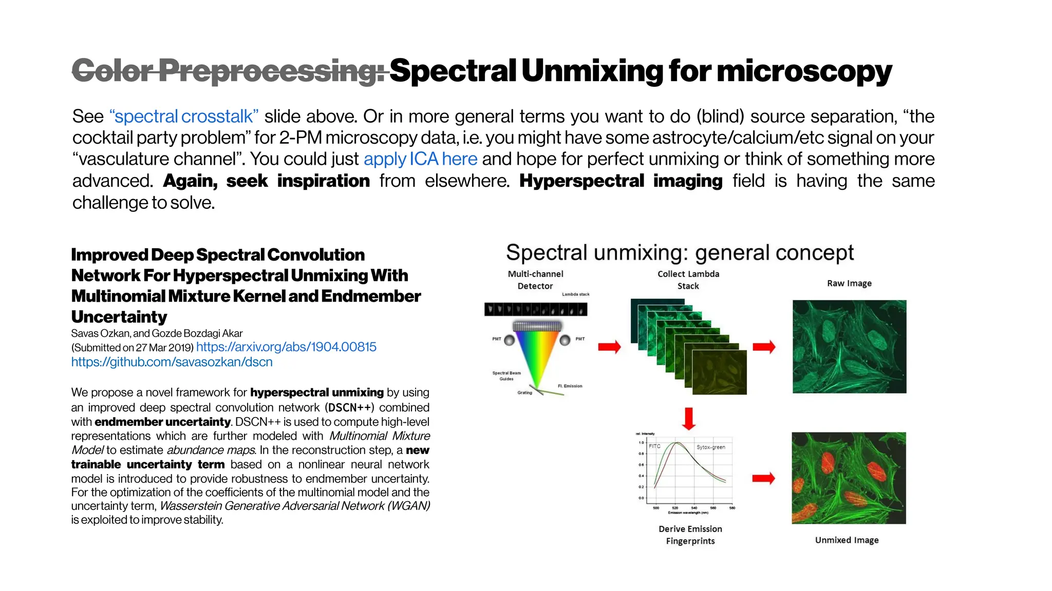
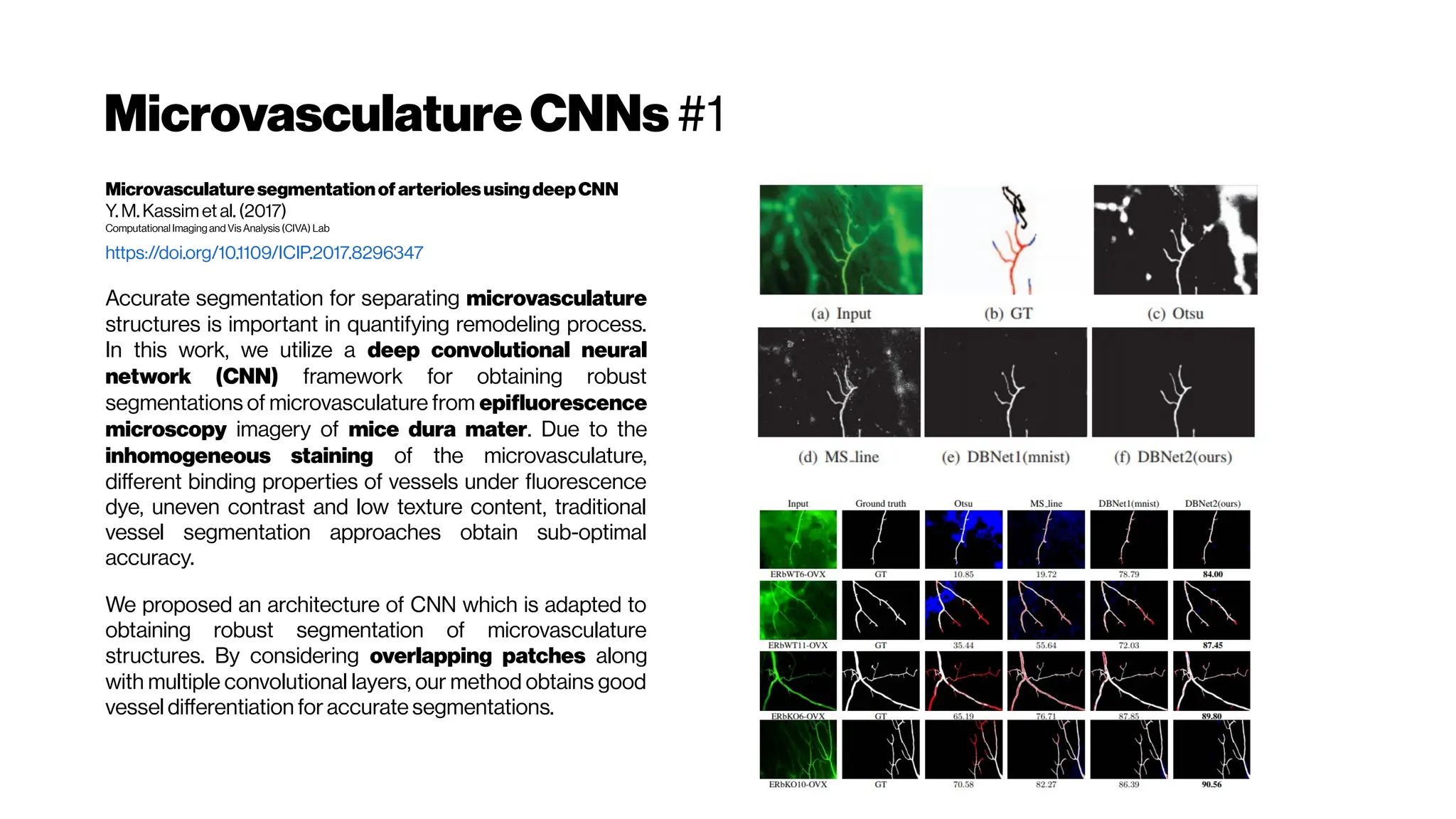
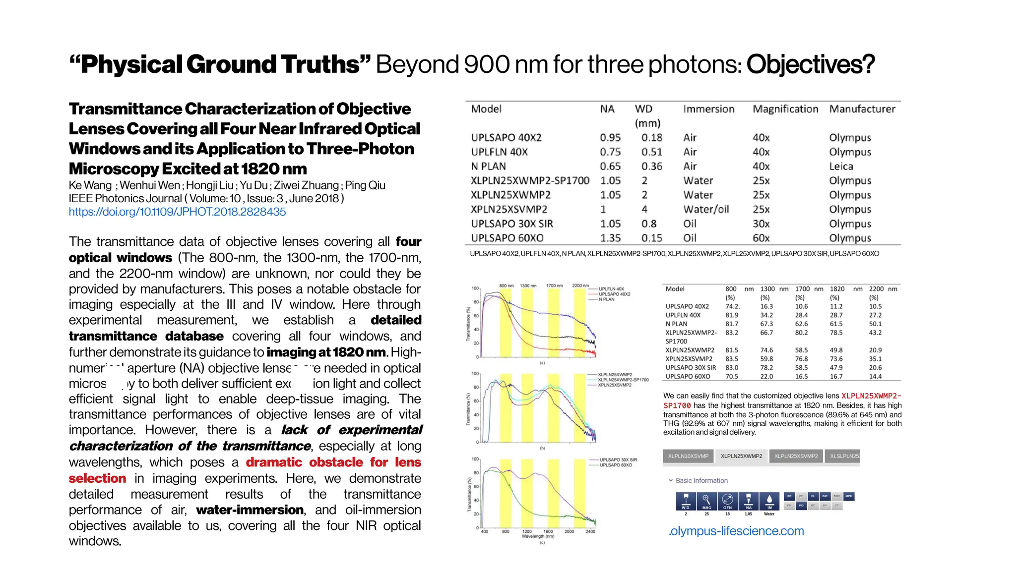
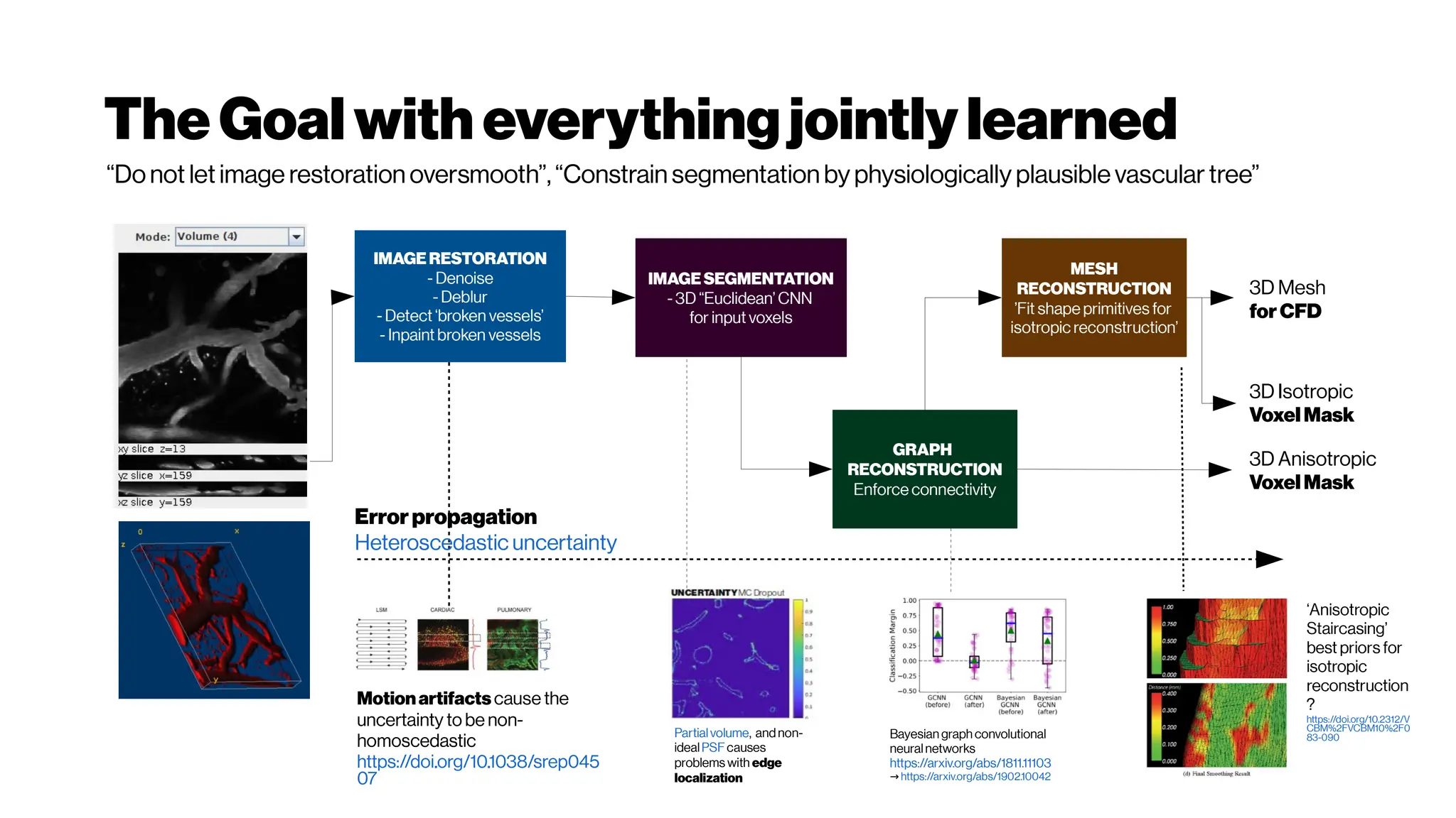
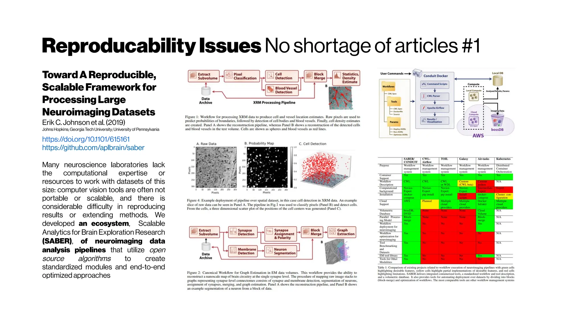
![MicrovasculatureCNNs #6: State-of-the-Art (SOTA)?
Deepconvolutionalneuralnetworksforsegmenting3Dinvivo
multiphotonimagesofvasculatureinAlzheimerdiseasemouse
modelsMohammad Haft-Javaherian, Linjing Fang,Victorine Muse, Chris B.
Schaffer, Nozomi Nishimura,Mert R.Sabuncu
Meinig Schoolof BiomedicalEngineering, Cornell University, Ithaca, NY, United States of America
March2019
https://doi.org/10.1371/journal.pone.0213539
https://arxiv.org/abs/1801.00880
Data: https://doi.org/10.7298/X4FJ2F1D (1.141 Gb)
Code: https://github.com/mhaft/DeepVess (Tensorflow / MATLAB)
We explored the use of convolutional neural networks to segment 3D vessels
within volumetric in vivo images acquired by multiphoton microscopy. We
evaluated different network architectures and machine learning
techniques in the context of this segmentation problem. We show that our
optimized convolutional neural network architecture with a customized loss
function, which we call DeepVess, yielded a segmentation accuracy that
was better than state-of-the-art methods, while also being orders of
magnitude fasterthan themanual annotation
While DeepVess offers very high accuracy in the problem we consider, there
is room for further improvement and validation, in particular in the
application to other vasiform structures and modalities. For example, other
types of (e.g., non-convolutional) architectures such as long short-term
memory (LSTM) can be examined for this problem. Likewise, a combined
approach that treats segmentation and centerline extraction methods
together, such as the method proposed by Bates etal. (2017) in a single
complete end-to-end learning framework might achieve higher centerline
accuracy levels.
Comparison ofDeepVess and the state-of-
the-art methods
3D rendering of (A) the expert’s
manual and
(B) DeepVess segmentation results.
Comparison ofDeepVess and the gold standard human
expertsegmentation results
We used 50% dropout during test-time [MCDropout] and
computed Shannon’s entropy for the segmentation
prediction at each voxel to quantify the uncertainty in
the automatedsegmentation.](https://image.slidesharecdn.com/multiphotonsegmentation2024-240117012649-7950e327/75/Two-Photon-Microscopy-Vasculature-Segmentation-102-2048.jpg)

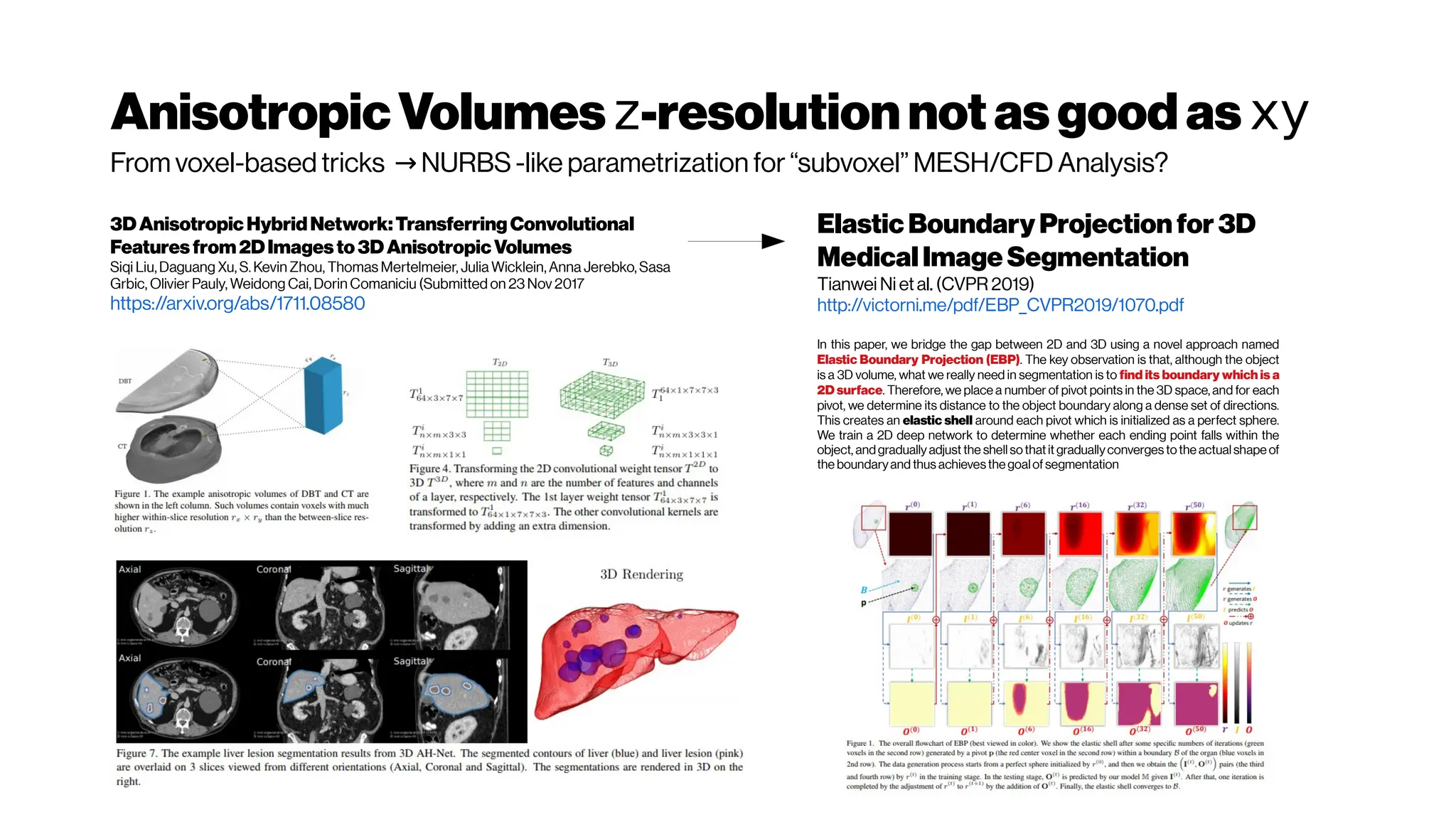
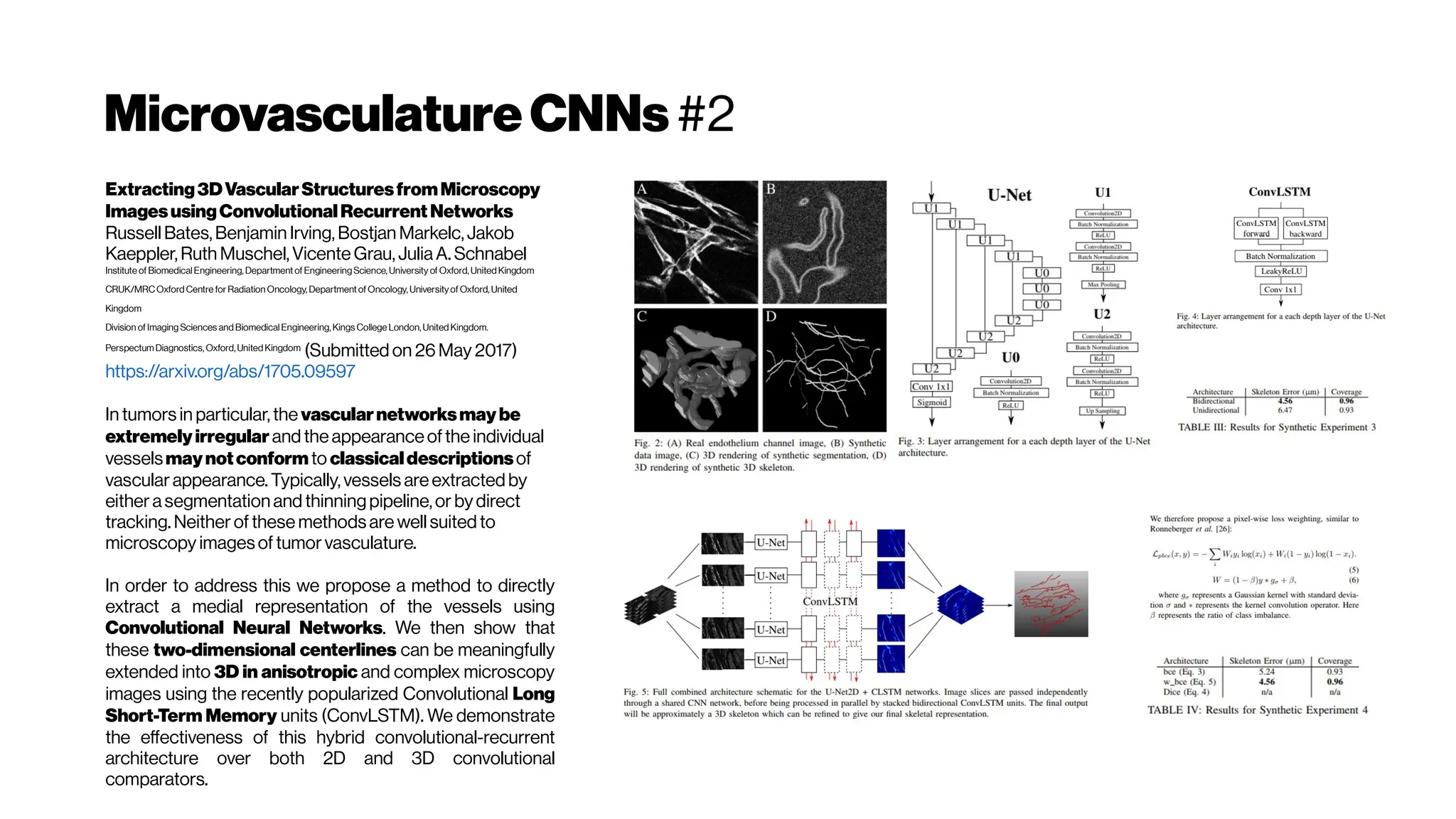
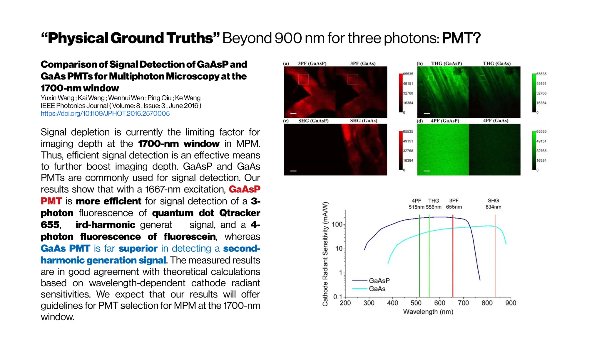
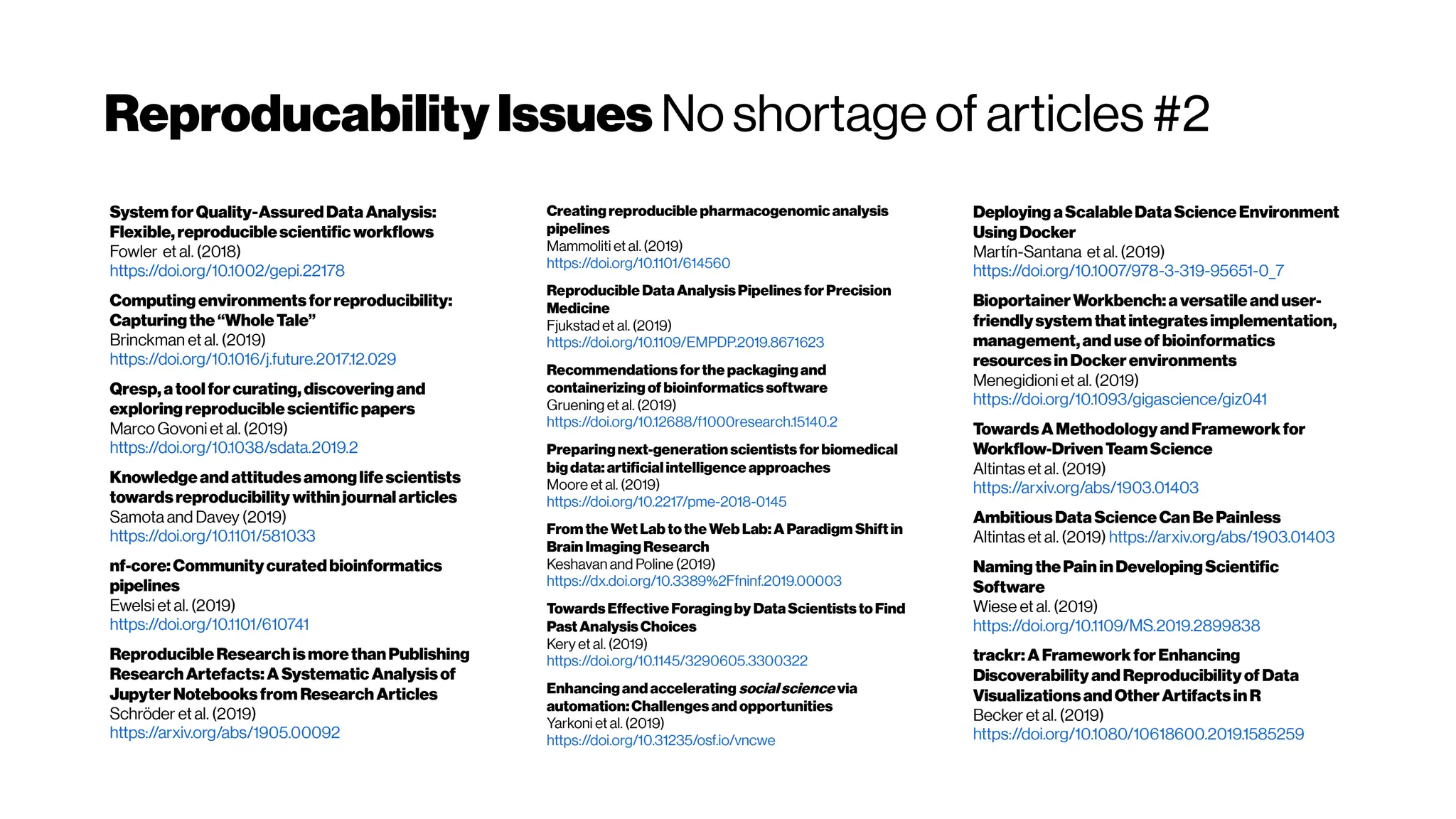
![WellwhatabouttheNOVELTYtoADD?
Depends a bit on what the
benchmarks reveal?
The DeepVess does not
seem out from this world in
terms of their specs so
possible to beat it with
“brute force”, by trying
different standard things
proposed in the literature
Keep this in mind, and
have a look on the
following slides
INPUT SEGMENTATION UNCERTAINTYMC Dropout
While DeepVess offers very high accuracy in the problem we consider,
there is room for further improvement and validation, in particular in the
application to other vasiform structures and modalities. For example, other
types of (e.g., non-convolutional) architectures such as long short-term
memory (LSTM) i.e. what the hGRU did
can be examined for this problem.
Likewise, a combined approach that treats segmentation and centerline
extraction methods together multi-task learning (MTL)
, such as the method
proposed by Bates et al. [25] in a single complete end-to-end learning
framework might achieve higher centerline accuracy levels.](https://image.slidesharecdn.com/multiphotonsegmentation2024-240117012649-7950e327/75/Two-Photon-Microscopy-Vasculature-Segmentation-105-2048.jpg)
![VasculatureNetworks Future
While DeepVess offers very high
accuracy in the problem we
consider, there is room for further
improvement and validation, in
particular in the application to other
vasiform structures and modalities.
For example, other types of (e.g.,
non-convolutional) architectures
such as long short-term memory
(LSTM) i.e. what the hGRU did
can be
examined for this problem. Likewise,
a combined approach that treats
segmentation and centerline
extraction methods together multi-task
learning (MTL)
, such as the method
proposed by Bates et al. [25] in a
single complete end-to-end
learning framework might achieve
higher centerline accuracy levels.
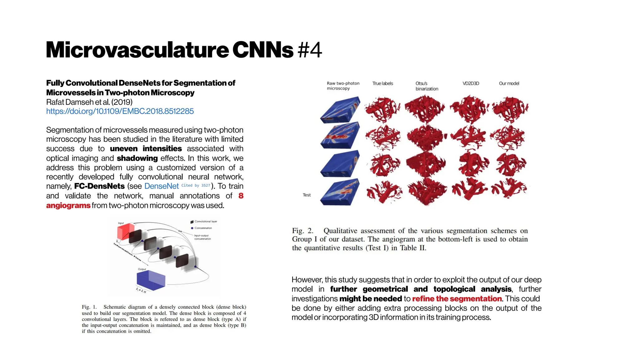
FC-DensNets
However, this study
suggests that in order
to exploit the output
of our deep model in
further geometrical
and topological
analysis, further
investigations might
be needed to refine
the segmentation.
This could be done
by either adding extra
processing blocks on
the output of the
model or
incorporating 3D
information in its
training process.
http://sci-hub.tw/10.1109
/jbhi.2018.2884678
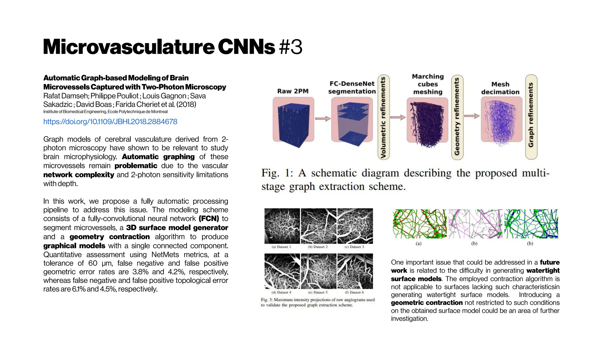
One important issue that could be
addressed in a future work is related
to the difficulty in generating
watertight surface models. The
employed contraction algorithm is
not applicable to surfaces lacking
such characteristics.](https://image.slidesharecdn.com/multiphotonsegmentation2024-240117012649-7950e327/75/Two-Photon-Microscopy-Vasculature-Segmentation-106-2048.jpg)


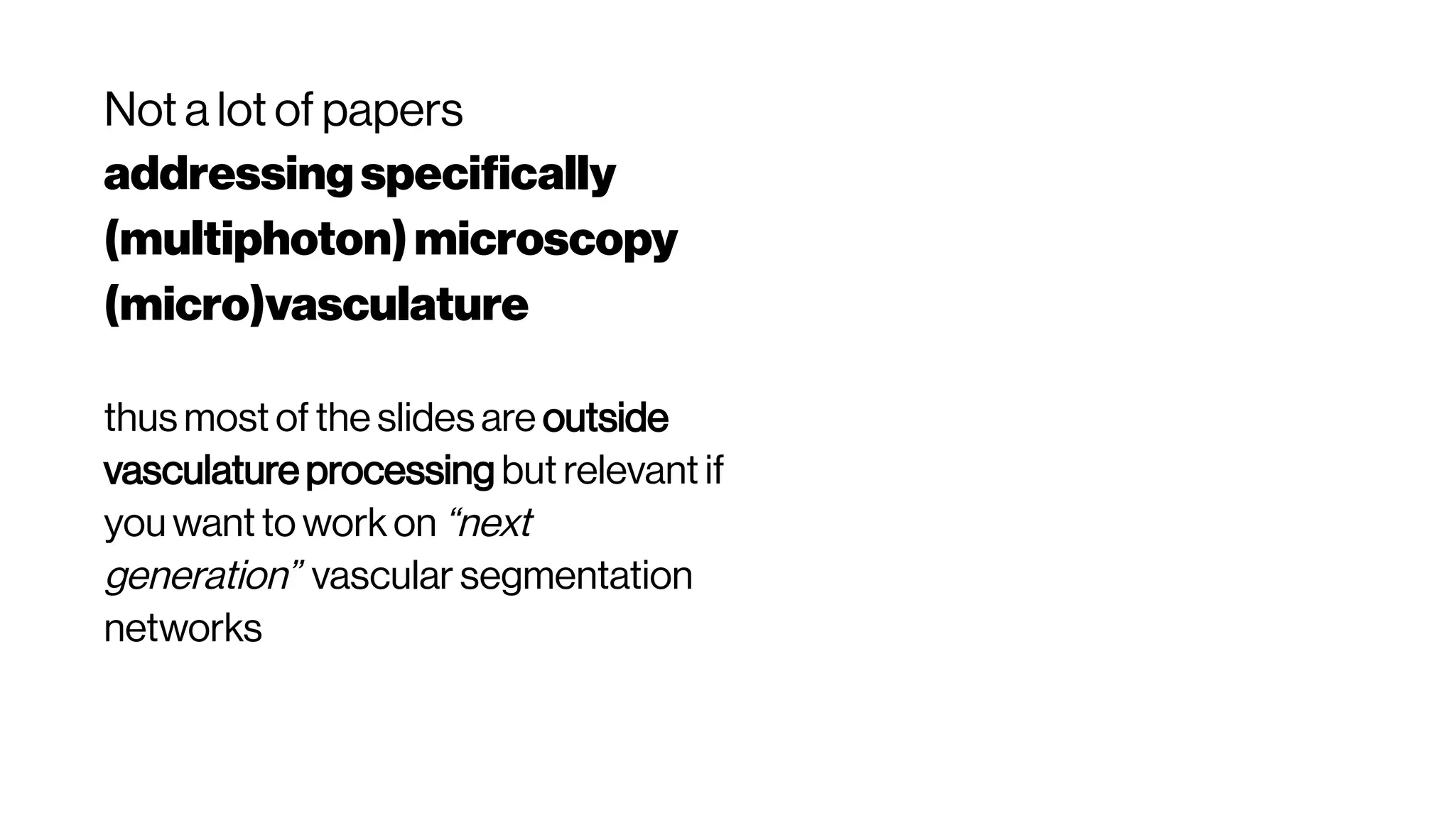
![Nicetohavesome realisticnoise-free2-PMvolumes/slices asbenchmarksfordenoising
performance evenifyouusethe‘statisticalnoisemodel’ approach
GRDN:GroupedResidualDenseNetworkforRealImageDenoising andGAN-
based Real-worldNoiseModeling
Dong-WookKim, Jae Ryun Chung, Seung-Won Jung
(Submitted on 27 May 2019) https://arxiv.org/abs/1905.11172
Toward real-world image denoising, there have been two main approaches. The first approach is to
find a better statistical model of real-world noise rather than the additive white Gaussian noise[e.g.
Brooks et al. 2018, Guo et al. 2018, Plötzand Roth 2018]
. In particular, a combination of Gaussian and Poisson
distributions was shown to closely model both signal-dependent and signal-independent noise.
The networks trained using these new synthetic noisy images demonstrated the superiority in
denoising real-world noisy images. One clear advantage of this approach is that we can have infinitely
many training image pairs by simply adding the synthetic noise to noise-free ground-truth images.
The second approach is thus in an opposite direction. From real-world noisy images, nearly noise-
freeground-truthimagescan be obtained by inverting an image acquisition procedure
We improve the previous GAN-based real-world noise simulation technique [Chen et al. 2018]
by including conditioning signals such as the noise-free image patch, ISO, and shutter speed as
additional inputs to the generator. The conditioning on the noise-free image patch can help
generating more realistic signal-dependent noise and the other camera parameters can increase
controllability and variety of simulated noise signals. We also change the discriminator of the previous
architecture [Chen et al. 2018] by using a recent relativistic GAN [Jolicoeur-Martineau 2018
Cited by 38
]. Unlike conventional GANs, the discriminator of the relativistic GAN learns to determine
which is morerealistic between real data and fake data
We thus plan to apply the proposed image denoising network to other image restoration tasks.
We also could not fully and quantitatively justify the effectiveness of the proposed real-world noise
modeling method. A more elaborate design is clearly necessary for better real-world noise
modeling. We believe that our real-world noise modeling method can be extended to other real-
worlddegradations such as blur, aliasing, and haze, which will be demonstratedin our future work](https://image.slidesharecdn.com/multiphotonsegmentation2024-240117012649-7950e327/75/Two-Photon-Microscopy-Vasculature-Segmentation-114-2048.jpg)
![If the image restoration is successful with the image segmentation
target, we could train another network for estimating image
quality and even optimize that in real-time in the 2-PM Setup [*]
?
[*]
Assuming that one has the time to acquire multiple times the same
slices if they are deemed sub-quality. Might work for histopathology,
butforanesthetized rodents?
Adeepneural networkforimagequalityassessment
Bosse et al. (2016) https://doi.org/10.1109/ICIP.2016.7533065
ExploitingUnlabeledData inCNNs bySelf-supervisedLearningto
Rank Xialei Liu et al. (2019) https://doi.org/10.1109/TPAMI.2019.2899857
JND-SalCAR:ANovelJND-basedSaliency-ChannelAttention
ResidualNetworkforImageQualityPrediction
Seo et al. (2016) https://arxiv.org/abs/1902.05316
Real-TimeQualityAssessmentofPediatricMRI viaSemi-
SupervisedDeepNonlocalResidualNeuralNetworks
Siyuan Liu et al. (2019) https://arxiv.org/abs/1904.03639
GANs-NQM:AGenerativeAdversarialNetworks basedNo
ReferenceQualityAssessmentMetricforRGB-DSynthesized
Views Suiyi Ling et al. (2019) https://arxiv.org/abs/1903.12088
Quality-awareUnpairedImage-to-ImageTranslation
Lei Chen et al. (2019) https://arxiv.org/abs/1903.06399](https://image.slidesharecdn.com/multiphotonsegmentation2024-240117012649-7950e327/75/Two-Photon-Microscopy-Vasculature-Segmentation-115-2048.jpg)
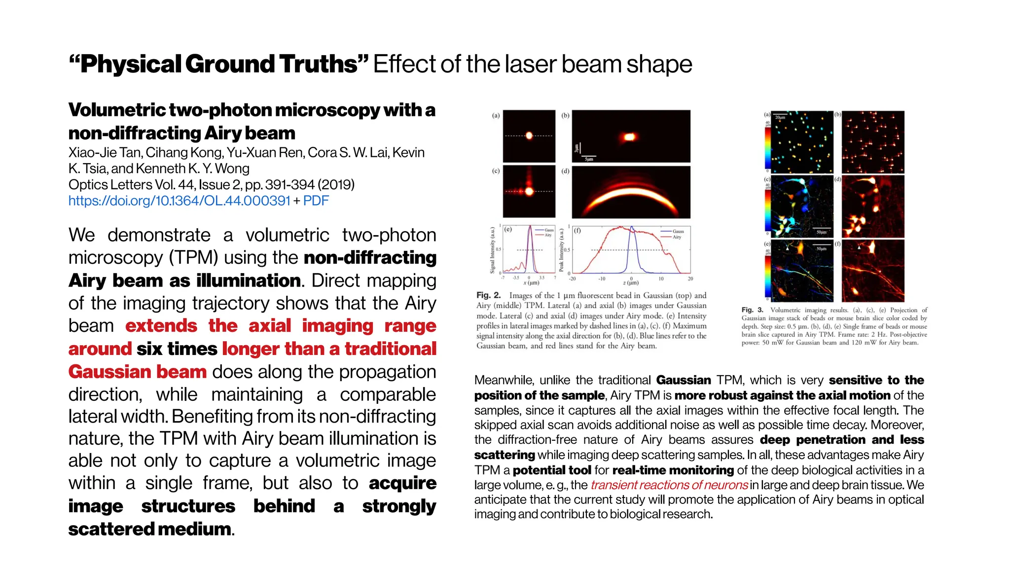
![HowaboutthePSFmodeling in2-PMsystems? For deblurring
OptimalMultivariateGaussianFittingforPSFModeling
inTwo-Photon Microscopy
Tim Tsz-Kit, Emilie Chouzenoux, Claire Lefort, Jean-Christophe Pesquet
http://doi.org/10.1109/ISBI.2018.8363621f
The mathematical representation of the light distribution of this spread phenomenon (of
infinitesimally pointsource) is well-known and described by the Point Spread Function
(PSF). The implementation of an efficient deblurring strategy often requires a
preliminary step of experimental data acquisition, aiming at modeling the PSF whose
shapedepends on the optical parameters of themicroscope.
The fitting model is chosen as a trade-off between its accuracy and its simplicity.
Several works in this field have been inventoried and specifically developed for
fluorescence microscopy [Zhang et al. 2007; Kirshner et al. 2012, 2013]
. In particular, Gaussian models
often lead to both tractable and good approximations of PSF [Anthonyand Granick2009;
Zhu and Zhang 2013]
. Although there exists an important amount of works regarding Gaussian
shape fitting [Hagen and Dereniak2008; Roonizi 2013]
, to the best of our knowledge, these techniques
remain limited to the 1D or 2D cases. Moreover, only few of them take into
account explicitly the presence of noise. Finally, a zero background value is usually
assumed (for instance, in the famous Caruanaet al. (1986) Cited by 46
’s approach). All the
aforementioned limitations severely reduce the applicability of existing methods for
processingreal3Dmicroscopy datasets.
In this paper, a novel optimization approach called FIGARO (FijiPlugin) has been
introduced for multivariate Gaussian shape fitting, with guaranteed convergence
properties. Experiments have clearly illustrated the applicative interest of FIGARO, in the
context of PSF identification in two-photon imaging. The versatility of FIGARO
makes it applicable to a wide range of applicative areas, in particular other microscopy
modalities.
The deblurringstepis performedusingthe OPTIMISMtoolboxfrom
Fiji](https://image.slidesharecdn.com/multiphotonsegmentation2024-240117012649-7950e327/75/Two-Photon-Microscopy-Vasculature-Segmentation-122-2048.jpg)
![Howmanyphotonsinpractice?
Adaptive optics in multiphoton microscopy:
comparison of two, three and four photon
fluorescenceDavid Sinefeld, Hari P. Paudel, Dimitre G. Ouzounov, Thomas
G. Bifano, and Chris Xu Optics Express Vol. 23, Issue 24, pp. 31472-31483 (2015)
https://doi.org/10.1364/OE.23.031472
We showed experimentally that the effect of aberrations on the signal increases
exponentially with the order of nonlinearity in a thick fluorescent sample.
Therefore, the impact of AO on higher order nonlinear imaging is much more dramatic.
We anticipate that the signal improvement shown here, will serve as a significant
enhancement to current 3PM, and perhaps for future 4PM systems, allowing
imagingdeeper and with betterresolution in biologicaltissues.
Phase correction for a 2-m-focallength cylindricallensfor 2-, 3- and 4- photon excited
fluorescence of Alexa Fluor 790, Sulforhodamine 101 and Fluorescein. (a) Left – 4-
photon fluorescence convergence curve showing a signal improvement factor of ×
320. Right – final phase applied on the SLM (b) left – 3-photon fluorescence
convergence curve showing a signal improvement factor of × 40. Right – final phase
applied on the SLM. (c) Left – 2-photon fluorescence convergence curve showing a
signalimprovement factor of×2.1.
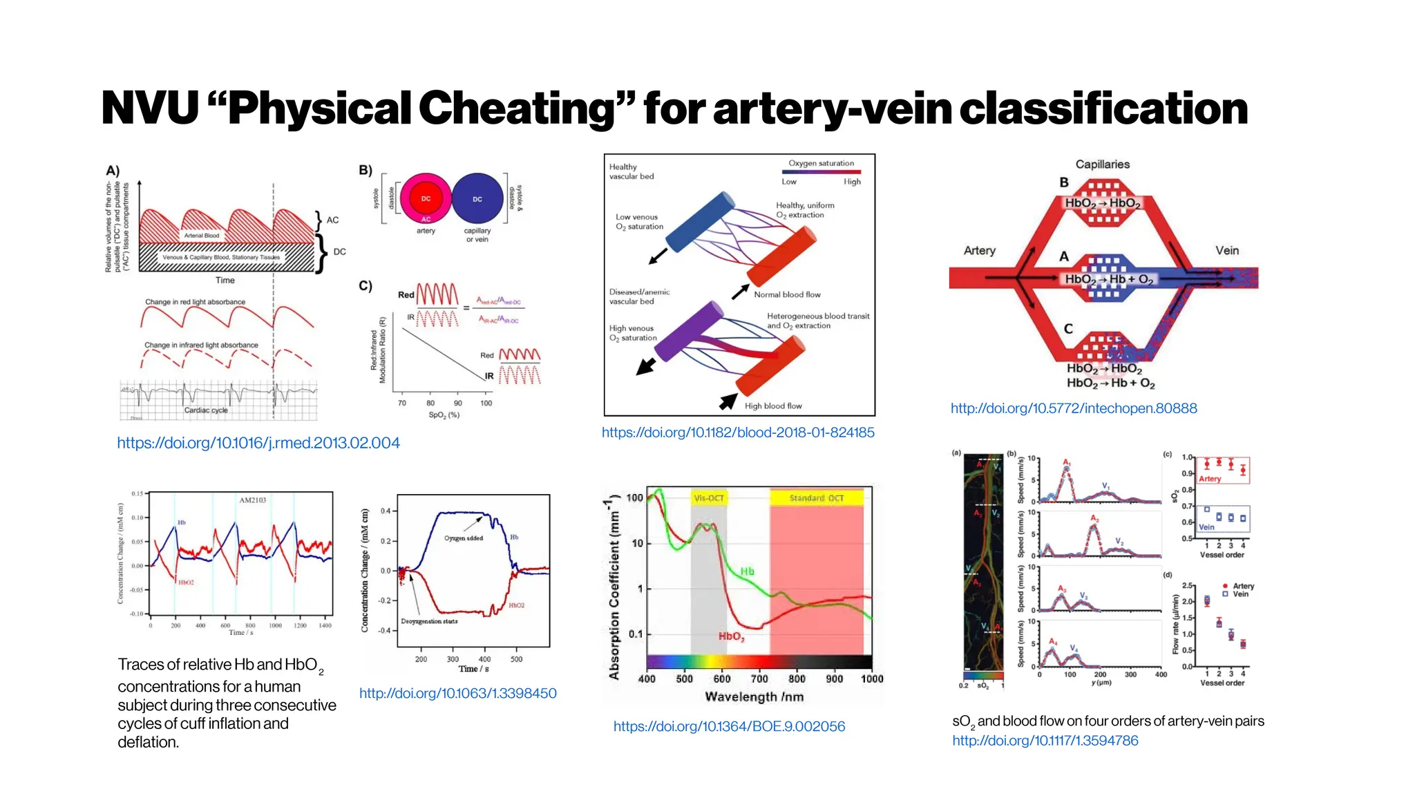
(left) The spectral response of oxygenated hemoglobin, deoxygenated hemoglobin,
and water as a function of wavelength. The red highlighted area indicates the
biological optical window where adsorption due to the body is at a minimum
Doane and Burda(2012)
(right) Wavelength-dependent attenuation length in brain tissue and
measured laser characteristics. Attenuation spectrum of a tissue model based on Mie
scattering and water absorption, showing the absorption length of water(la, blue dashed
line), the scattering length of mouse brain cortex (ls, red dashed-dotted line), and the
combined effective attenuation length (le, green solid line). The red stars indicate
the attenuation lengths reported for mouse cortex in vivo from previous work[Kobat et al., 2009]
.
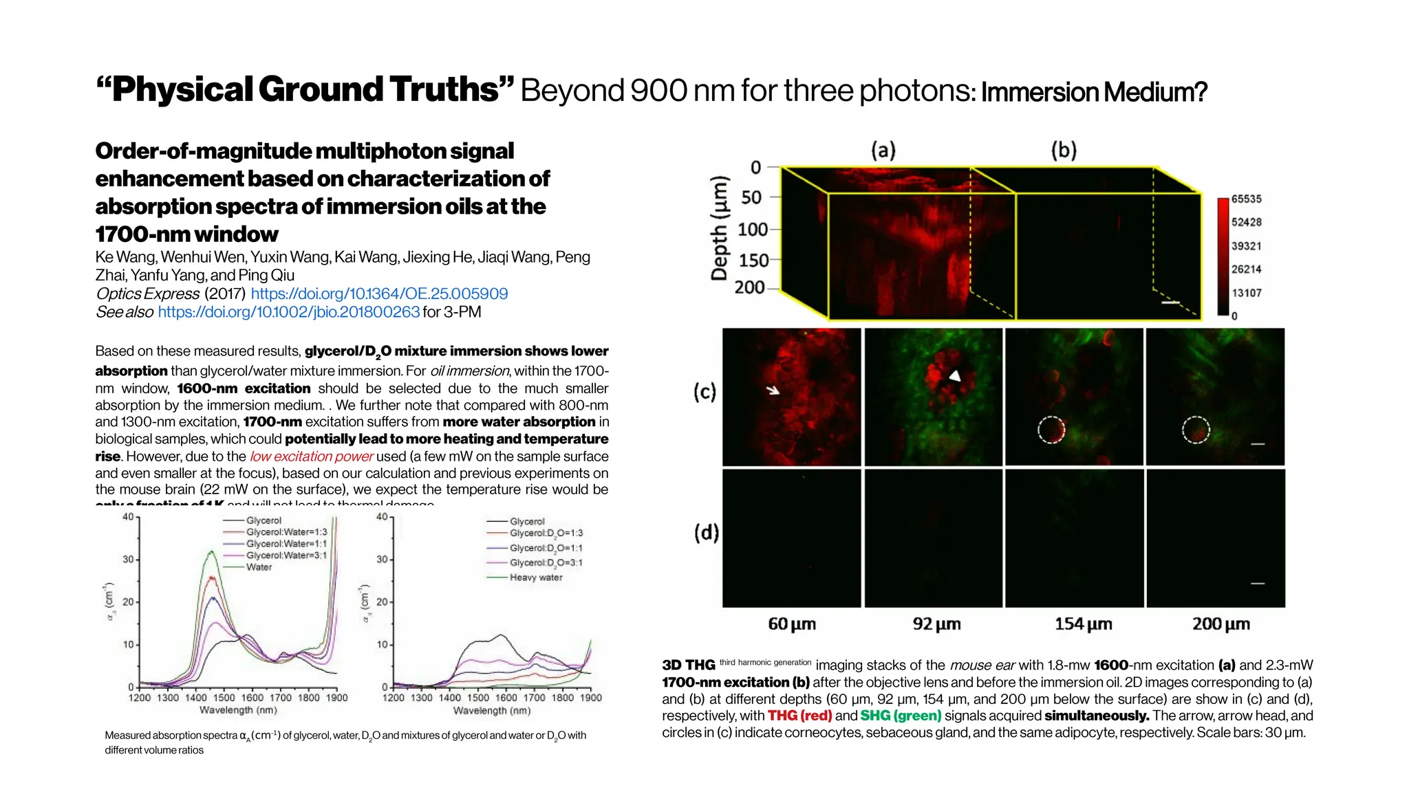
The figure hows that the optimum wavelength window (for three-photon microscopy) in
terms of tissue penetration is near 1,700 nm when both tissue scattering and absorption
areconsidered. Horton et al. (2013)
Why not4-PM ifthesectioningimproveswithincreased
nonlinearorder?There are spectral absorbers in the brain,
“near-infrared” (NIR) optical windows for optimal wavelengths](https://image.slidesharecdn.com/multiphotonsegmentation2024-240117012649-7950e327/75/Two-Photon-Microscopy-Vasculature-Segmentation-133-2048.jpg)


![Dice? Agood “medicalmetric”for us? AVD?
Metricsforevaluating3D
medicalimagesegmentation:
analysis,selection,andtool.
Abdel Aziz Taha andAllan Hanbury TUWien
BMC Medical Imaging 2015 15:29
https://doi.org/10.1186/s12880-015-0068-x
https://github.com/Visceral-Project/EvaluateSegmentati
on
Since metrics have different properties (biases, sensitivities),
selecting suitable metrics is not a trivial task. This paper
provides analysis of the 20 implemented metrics, in particular
of their properties, and suitabilities to evaluate segmentations,
given particular requirements and segmentations with particular
properties.
The Dice coefficient [Dice 1945] (DICE), also called the
overlap index, is the most used metric in validating medical
volume segmentations. In addition to the direct comparison
between automatic and ground truth segmentations, it is
common to use the DICE to measure reproducibility
(repeatability). Zou et al. 2004 used the DICE as a measure of
the reproducibility as a statistical validation of manual annotation
where segmenters repeatedly annotated the same MRI image.
Contour is important: Depending on the individual task, the
contour can be of interest, that is the segmentation algorithms
should provide segments with boundary delimitation as exact as
possible. Metrics that are sensitive to point positions (e.g. HD
and AVD) are more suitable to evaluate such segmentation than
others. Volumetric similarity VS is to be avoided in this case.
TheHausdorffDistance(HD) is generally sensitivetooutliers.
Because noiseandoutliers arecommon in medical segmentations, itis
not recommended to use theHD directly [Zhang and Lu2004].
TheAverageDistance,ortheAverageHausdorffDistance(AVD),
is the HD averaged over all points. TheAVD is known tobe stableand
less sensitiveto outliers than theHD. Itis defined by:
The Hausdorff distance (HD) and the
average Hausdorff distance (AVD) are based
on calculating the distances between all pairs
of voxels. This makes them
computationally very intensive,
especially with large images. herefore, to
efficiently calculate the AVD, we use a
modified version of the nearest neighbor
(NN) algorithm proposed by
Zhao et al. 2014 in which a 3D cell grid is built
on the point cloud.](https://image.slidesharecdn.com/multiphotonsegmentation2024-240117012649-7950e327/75/Two-Photon-Microscopy-Vasculature-Segmentation-165-2048.jpg)
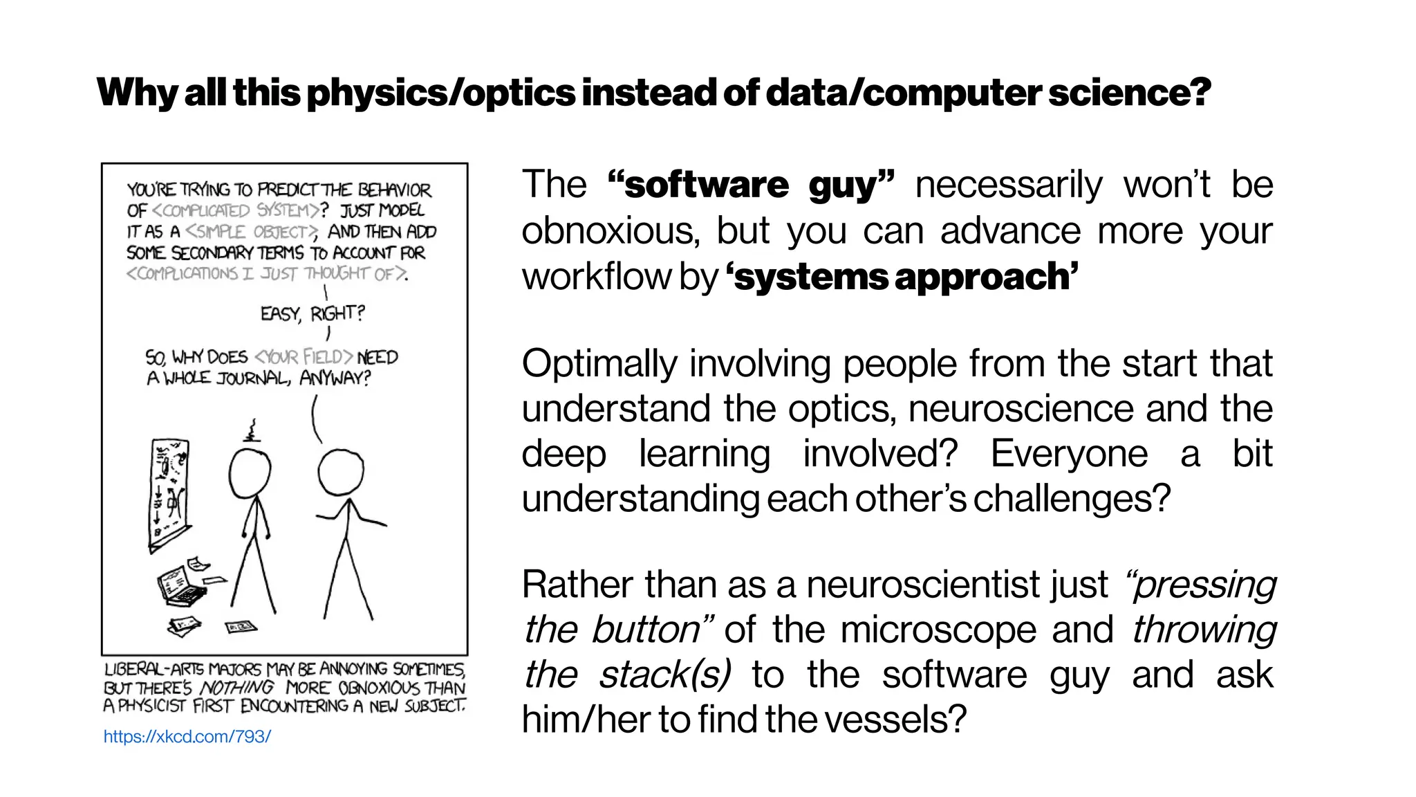
![UQAleatoric vs. Epistemic uncertainty?
https://github.com/yaringal/ConcreteDropout/blob/master/concrete-dropout-keras.ipynb:
D = 1
K_test = 20 # “draw” K times, 20 inferences
MC_samples = np.array([model.predict(X_val) for _ in range(K_test)])
means = MC_samples[:, :, :D] # K x N
epistemic_uncertainty = np.var(means, 0).mean(0)
logvar = np.mean(MC_samples[:, :, D:], 0)
aleatoric_uncertainty = np.exp(logvar).mean(0)
https://arxiv.org/abs/1705.07832:
Three types of uncertainty are often encountered in Bayesian modelling.
Epistemic (known also as ‘uncertainty’)
uncertainty captures our ignorance about the
models most suitable to explain our data; Aleatoric (known also as ‘risk’)
uncertainty
captures noise inherent in the environment (remember aleajactaest); Lastly,
predictiveuncertainty conveys the model’s uncertainty in its output.
Epistemic uncertainty reduces as the amount of observed data increases—
hence its alternative name “reducible uncertainty”. Aleatoric uncertainty
captures noise sources such as measurement noise—noises which cannot be
explained away even if more data were available (although this uncertainty can
be reduced through the use of higher precision sensors for example). This
uncertainty is often modelled as part of the likelihood, at the top of the model,
where we place some noise corruption process on the function’s output.
Combining both types of uncertainty gives us the predictive uncertainty—the
model’s confidence in its prediction, taking into account noise it can explain
away and noise it cannot. This uncertainty is often obtained by generating
multiple functions from our model and corrupting them with noise (with
precision τ ).
For some critique of this, see the discussion:
Posted by u/sschoener 1 year ago (2018)
[D] What isthe current state of dropout asBayesianapproximation?
https://www.reddit.com/r/MachineLearning/comments/7bm4b2/d_what_is_the_current_state_of_dropout_as/
with Ian Osband, DeepMind @IanOsband Alternative?
→ https://arxiv.org/abs/1806.03335
WhatUncertaintiesDoWeNeedinBayesianDeep Learningfor
ComputerVision?Alex Kendall, Yarin Gal
https://arxiv.org/abs/1703.04977
In (d) our model exhibits increased aleatoric uncertainty on object boundaries and for objects far from
the camera. Epistemic uncertainty accounts for our ignorance about which model generated our
collected data. This is a notably different measure of uncertainty and in (e) our model exhibits
increased epistemic uncertainty for semantically and visually challenging pixels. The bottom row
shows a failure case of the segmentation model when the model fails to segment the footpath due to
increasedepistemicuncertainty, but not aleatoric uncertainty.](https://image.slidesharecdn.com/multiphotonsegmentation2024-240117012649-7950e327/75/Two-Photon-Microscopy-Vasculature-Segmentation-175-2048.jpg)
![Subject-wiseCalibrationIssues?Ensemblesthenicest
AssessingReliability and
ChallengesofUncertainty
EstimationsforMedicalImage
Segmentation
Alain Jungo, Mauricio Reyes (Submitted on 7 Jul 2019)y
https://arxiv.org/abs/1907.03338
https://github.com/alainjungo/reliability-challenges-uncertain
ty
Although many uncertainty estimation methods
have been proposed for deep learning, little is known
on their benefits and current challenges for medical
image segmentation. Therefore, we report results of
evaluating common voxel-wise uncertainty measures
with respect to their reliability, and limitations on two
medical image segmentation datasets. Results show
that current uncertainty methods perform similarly and
although they are well-calibrated at the dataset level,
they tend to be miscalibrated at subject-level.
Therefore, the reliability of uncertainty estimates is
compromised, highlighting the importance of
developing subject-wise uncertainty estimations.
Additionally, among the benchmarked methods, we
found auxiliary networks to be a valid alternative to
common uncertainty methods since they can be
applied toany previously trainedsegmentation model.
Unsurprisingly, the ensemble method yields rank-wise the most
reliable results (Tab. 1) and would typically be a good choice (if the
resources allow it). The results also revealed that methods based on MC
dropout are heavily dependent on the influence of dropout on the
segmentation performance. In contrast, auxiliary networks turned out
to be a promising alternative to existing uncertainty measures.
They perform comparable to other methods but have the benefit of being
applicable to any high-performing segmentation network not optimized
to predict reliable uncertainty estimates. No significant differences were
found between using auxiliary feat. and auxiliary segm.. Through a
sensitivity analysis performed over all studied uncertainty methods, we
could confirm our observations that different uncertainty estimation
methodsyielddifferentlevelsofprecision andrecall.
Furthermore, we observed that when using current uncertainty methods
for correcting segmentations, a maximum benefit can be attained
when preferring a combination of low precision segmentation
modelsanduncertainty-basedfalsepositive removal.
Our evaluation has several limitations worth mentioning. First, although
the experiments were performed on two typical and distinctive datasets,
they feature large structures to segment. The findings reported herein
may differ for other datasets, especially if these consists of very small
structures to be segmented. Second, the assessment of the
uncertainty is influenced by the segmentation performance. Even though
we succeeded in building similarly performing models, their differences
cannotbefully decoupled andneglectedwhen analyzingthe uncertainty.
Overall, we aim with these results to point to the existing challenges for a
reliable utilization of voxel-wise uncertainties in medical image
segmentation, and foster the development of subject/patient-level
uncertainty estimation approaches under the condition of HDLSS.
We recommend that utilization of uncertainty methods ideally need to be
coupled with an assessment of model calibration at the subject/patient-
level. Proposed conditions, along with the threshold-free ECE metric
can be adopted to test whether uncertainty estimations can be of benefit
for a given task.
Ensembles. Another way of quantifying uncertainties is by ensembling
multiple models [Lakshminarayanan etal. 2017]. We combined the class
probabilities over all K = 10 networks and used the normalized entropy as
uncertainty measure. The individual networks share the same architecture
but were trained on different subsets (90%) of the training dataset and
different randominitialization to enforcevariability.
Auxiliary network. Inspired by [DeVriesandTaylor2018;
Robinson et al. 2018], where an auxiliary network is used to predict
segmentation performance at the subject-level, we apply an auxiliary
network to predict voxel-wise uncertainties of the segmentation model by
learning from the segmentation errors (i.e., false positives and false
negatives). For the experiments, we considered two opposing types of
auxiliary networks. The first one, named auxiliary feat., consists of
three consecutive 1×1 convolution layers cascaded after the last feature
maps of the segmentation network. The second auxiliary network, named
auxiliary segm., is a completely independent network (same U-Net as
described in Sec. 2.2) that uses as input the original images and the
segmentation masks produced by the segmentation model (generated by
five-fold cross-validation). We normalized the output uncertainty subject-
wise to[0, 1]for comparability purposes](https://image.slidesharecdn.com/multiphotonsegmentation2024-240117012649-7950e327/75/Two-Photon-Microscopy-Vasculature-Segmentation-177-2048.jpg)
![BrierScorebetterthanROCAUCforclinicalutility? Yes,but...
…Stillsensitivetodiseaseprevalence
TheBrierscoredoesnotevaluatetheclinicalutilityof
diagnostictestsorpredictionmodels
Melissa Assel, DanielD. SjobergandAndrew J. Vickers
MemorialSloan KetteringCancerCenter,NewYork,USA
Diagnostic andPrognostic Research 2017 1:19 https://doi.org/10.1186/s41512-017-0020-3
The Brier score is an improvement over other statistical performance measures, such as
AUC, because it is influenced by both discrimination and calibration simultaneously, with
smaller values indicating superior model performance. The Brier score also estimates a well-
defined parameter in the population, the mean squared distance between the observed and
expected outcomes. The square root of the Brier score is thus the expected distance between
the observed andpredicted value on the probability scale.
However, the Brier score is prevalence dependent i.e. sensitive to class imbalance in machine learning jargon
in such a
way that the rank ordering of tests or models may inappropriately vary by prevalence [
Wu andLee 2014]. For instance, if a disease was rare (low prevalence), but very serious and easily
cured by an innocuous treatment (strong benefit to detection), the Brier score may
inappropriately favor a specific test compared to one of greater sensitivity. Indeed, this is
approximately what was seen in the Zikavirus paper [Braga et al. 2017]
We advocate, as an alternative, the use of decision-analytic measures such as net benefit.
Net benefit always gave a rank ordering that was consistent with any reasonable evaluation of
the preferable test or model in a given clinical situation. For instance, a sensitive test had a
higher net benefit than a specific test where sensitivity was clinically important. It is
perhaps not surprising that a decision-analytic technique gives results that are in accord with
clinical judgment because clinical judgment is “hardwired” into the decision-analytic statistic.
That said, this measure is not without its own limitations, in particular, the assumption that the
benefit and harms of treatment do not vary importantly between patients independently of
preference.
Howshouldweevaluatepredictiontools?Comparisonof
threedifferenttools forpredictionofseminalvesicle
invasionatradicalprostatectomy as atestcase
Giovanni Lughezzani et al. Eur Urol. 2012 Oct; 62(4): 590–596.
https://dx.doi.org/10.1016%2Fj.eururo.2012.04.022
Traditional (area-under-the-receiver-operating-characteristic-
curve (AUC), calibration plots, the Brier score, sensitivity and
specificity, positive and negative predictive value) and novel (risk
stratification tables, the net reclassification index, decision curve
analysis and predictiveness curves) statistical methods quantified
the predictiveabilities ofthethreetested models.
Traditional statistical methods (receiver operating characteristic
(ROC) plots and Brier scores), as well as two of the novel
statistical methods (risk stratification tables and the net
reclassification index) could not provide clear distinction
between the SVI prediction tools. For example, receiver
operating characteristic (ROC) plots and Brier scores seemed
biased against the binary decision tool (ESUO criteria) and gave
discordant results for the continuous predictions of the Partin
tables and the Gallina nomogram. The results of the calibration
plots were discordant with thoseof the ROC plots. Conversely, the
decision curve clearly indicated that the Partin tables (
Zorn et al. 2009) represent the ideal strategy for stratifying
theriskof seminal vesicleinvasion(SVI).](https://image.slidesharecdn.com/multiphotonsegmentation2024-240117012649-7950e327/75/Two-Photon-Microscopy-Vasculature-Segmentation-180-2048.jpg)
![NoisyLabels as ‘annotator confusion’
Learning FromNoisyLabelsBy Regularized EstimationOf
AnnotatorConfusion
Ryutaro Tanno, Ardavan Saeedi, Swami Sankaranarayanan, DanielC. Alexander, NathanSilberman
UniversityCollegeLondon, UK;ButterflyNetwork,NewYork,USA
Submitted on 10Feb 2019https://arxiv.org/abs/1902.03680
The predictive performance of supervised learning algorithms depends on the quality of labels. In a
typical label collection process, multiple annotators provide subjective noisy estimates of the "truth"
under the influence of their varying skill-levels and biases. Blindly treating these noisy labels as the
ground truth limits the accuracy of learning algorithms in the presence of strong disagreement. This
problem is critical for applications in domains such as medical imaging where both the annotation
cost and inter-observer variability are high. In this work, we present a method for simultaneously
learning the individual annotator model and the underlying true label distribution, using only noisy
observations. Each annotator is modeled by a confusionmatrix that is jointly estimated along with the
classifier predictions. We propose to add a regularization term to the loss function that encourages
convergence to the true annotator confusion matrix. We provide a theoretical argument as to how the
regularization is essential to ourapproach both forthecaseofsingleannotatorand multiple annotators.
Future work shall consider imposing structures on the confusion matrices to broaden up the
applicability to massively multi-class scenarios e.g. introducing taxonomy based sparsity [
Van Horn 2018] and low-rankapproximation. We also assumed that thereisonlyonegroundtruth
for each input; this no longer holds true when the input images are truly ambiguous—recent
advances in modelling multi-modality of label distributions [Saeedi etal.2017, Kohl et al. 2018]
potentially facilitate relaxation of such assumption. Another limiting assumption is the image
independence of the annotator’s label noise. The majority of disagreement between annotators
arise in the difficult cases. Integrating such input dependence of label noise [Raykar et al. 2009,
Xiaoet al. 2015] is also avaluablenextstep.](https://image.slidesharecdn.com/multiphotonsegmentation2024-240117012649-7950e327/75/Two-Photon-Microscopy-Vasculature-Segmentation-183-2048.jpg)
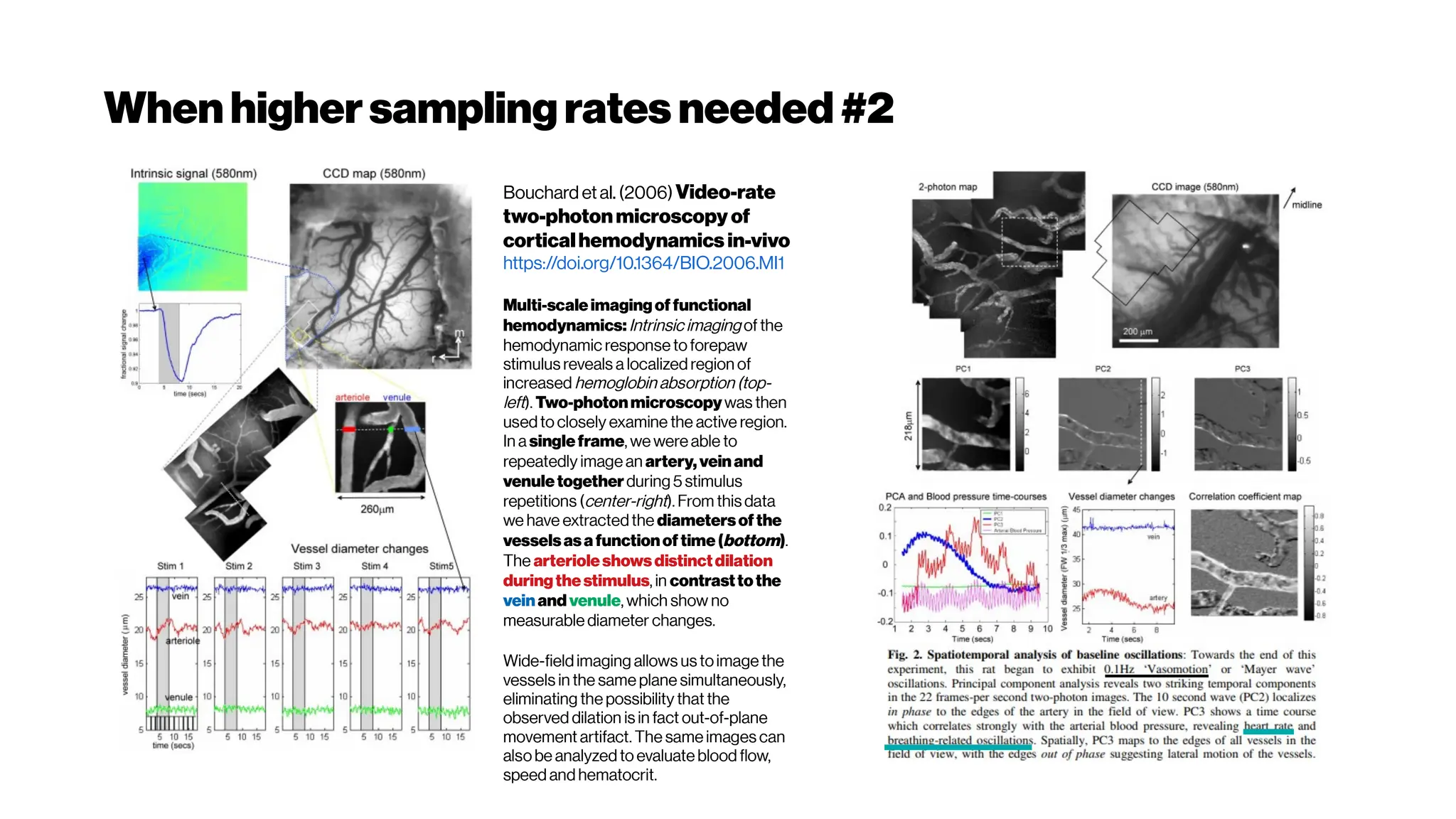
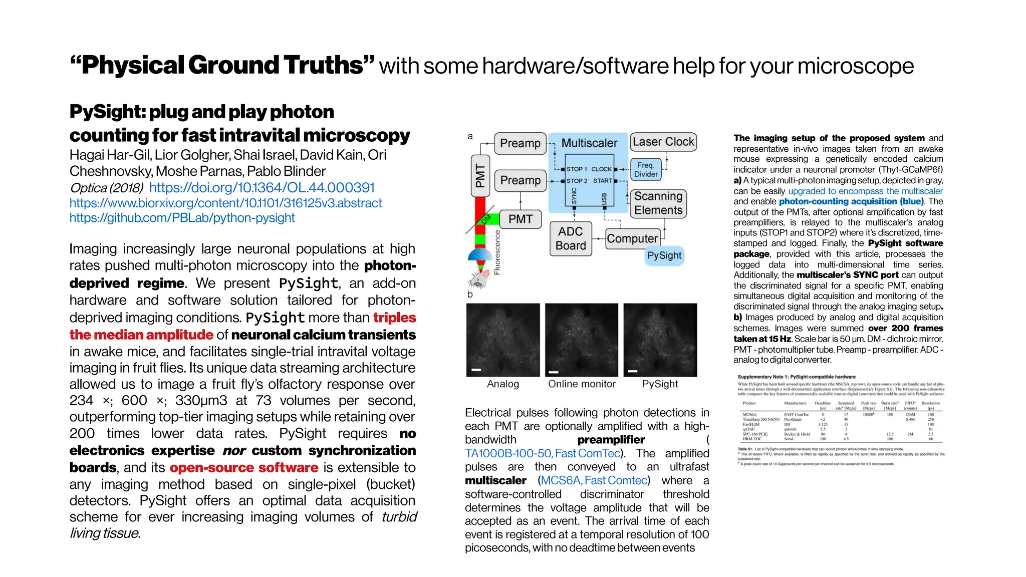
![Whenhigher samplingrates needed: Your dyes willbe tooslow alsoat some point
Whole brain, single-cell resolution calcium transients captured with light-sheet
microscopy (Ahrens et al. [118]). (A) Two spherically focused beams rapidly swept out a
four-micron-thick plane orthogonal to the imaging axis. The beam and objective step
together along the imaging axis to build up three-dimensional volume image at 0.8Hz (B).
(C) Rapid light-sheet imaging of GCaMP5G calcium transients revealed a specific
hindbrain neuron population (D, green traces) traces correlated with spinal cord neuropil
activity(black trace).
Schultz et al. 2016 https://doi.org/10.1101/036632](https://image.slidesharecdn.com/multiphotonsegmentation2024-240117012649-7950e327/75/Two-Photon-Microscopy-Vasculature-Segmentation-204-2048.jpg)
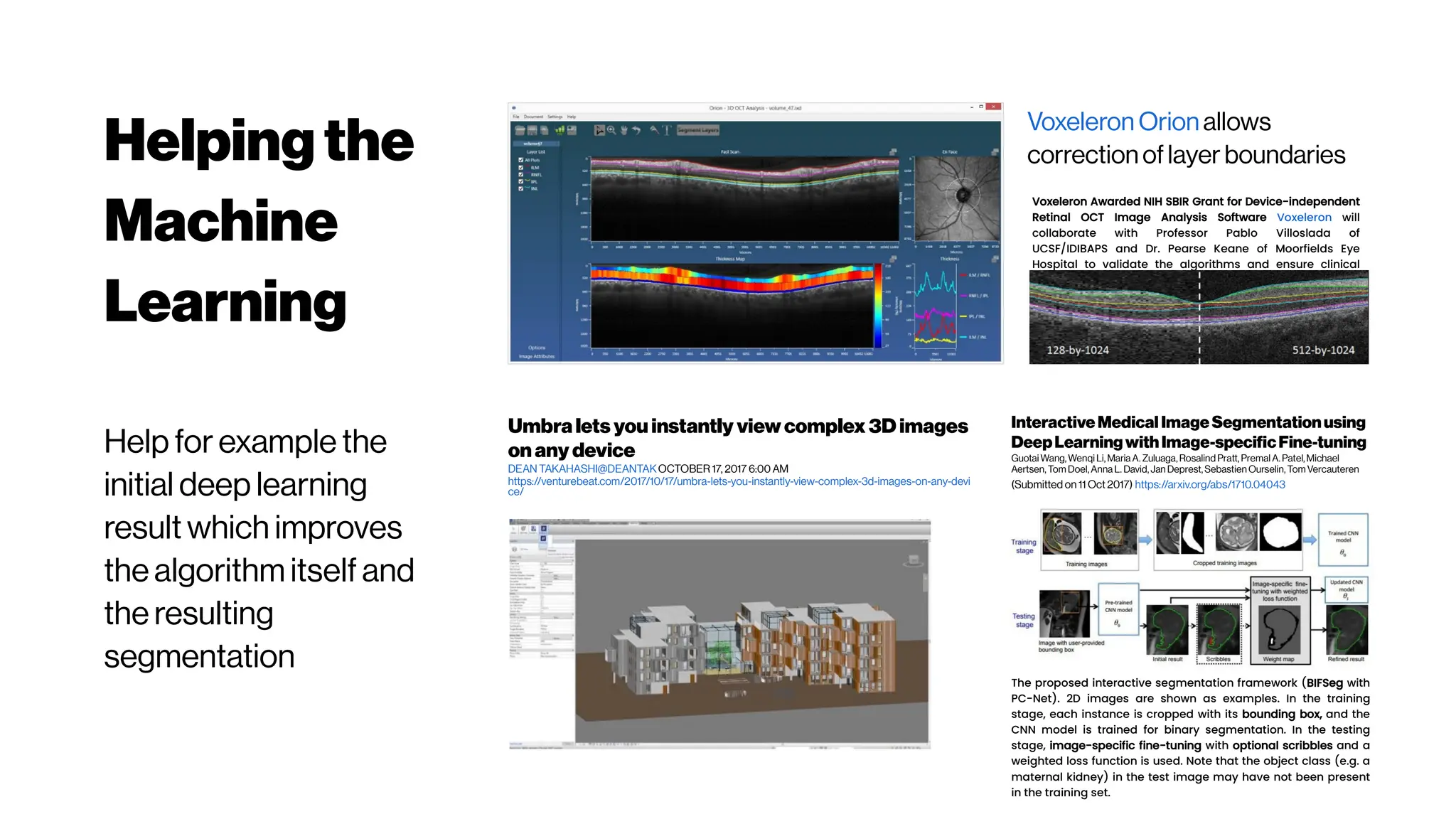

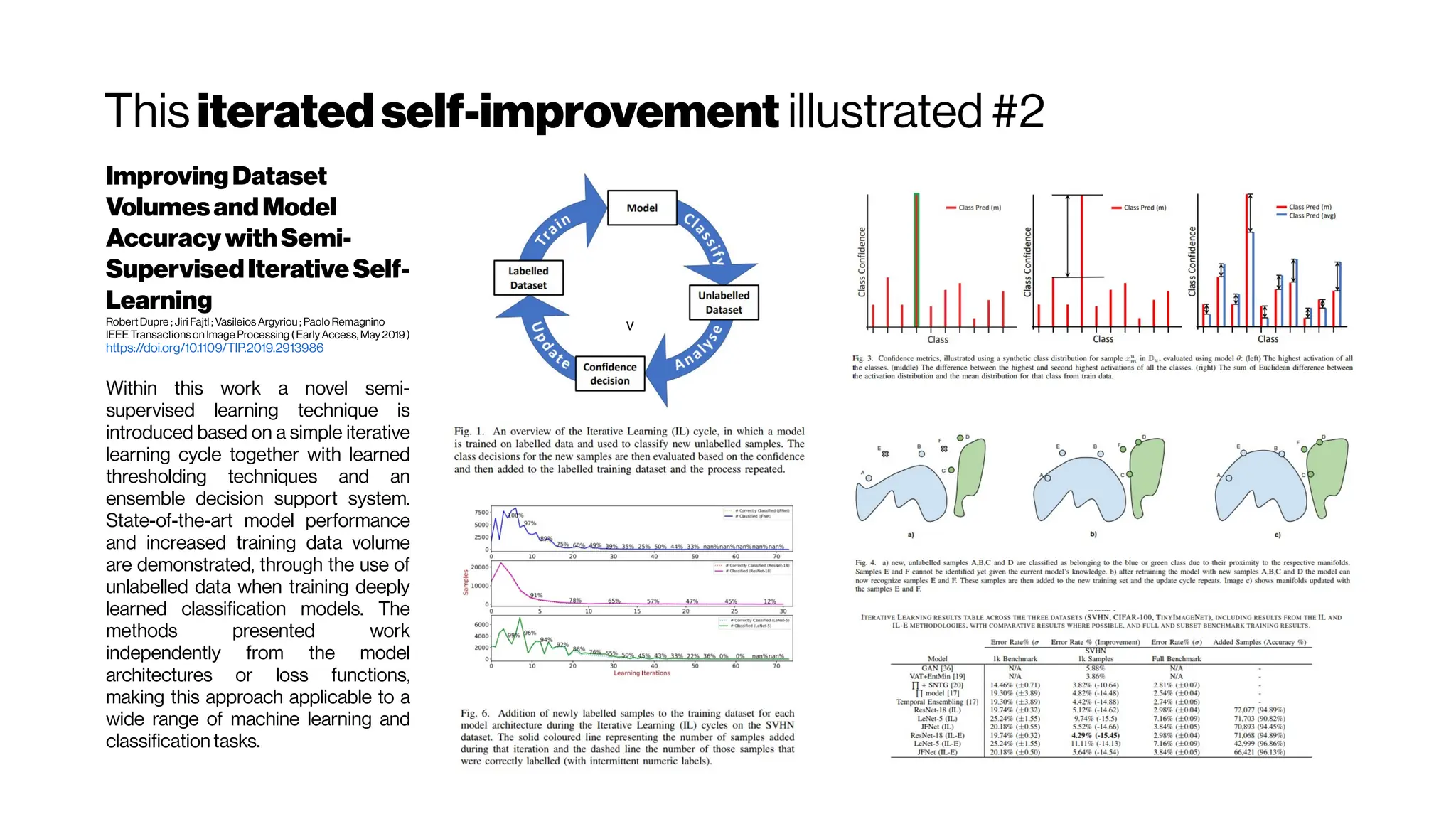
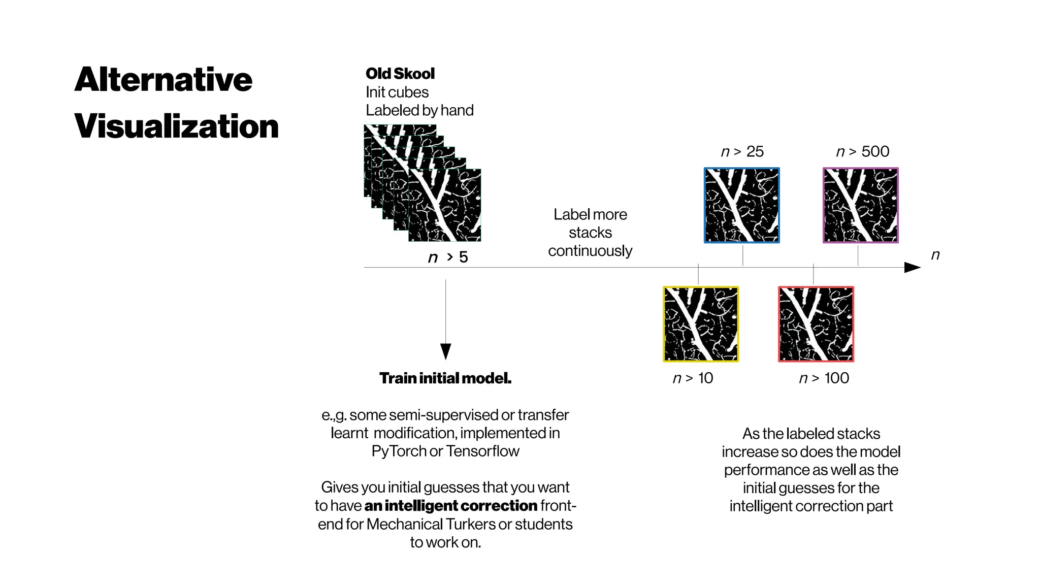


This document discusses using deep learning for automated segmentation of 3D vasculature stacks from multiphoton microscopy images. It highlights relevant literature on semi-supervised U-Net architectures that can leverage both labeled and unlabeled data. The document notes the lack of robust automated tools for large datasets and recommends taking inspiration from electron microscopy segmentation. It provides an overview of a presentation on vasculature segmentation using deep learning, covering basic concepts, recent papers, and "history of ideas" in the field to provide inspiration for new projects.


![[DSC Europe 25] Jovan Bogicevic - Legacy to AI-Driven Defense: Transforming D...](https://cdn.slidesharecdn.com/ss_thumbnails/rsarluadt563hntyfc8q-3-251211083849-3e7bc4c0-thumbnail.jpg?width=640&height=640&fit=bounds)
![[DSC Europe 25] Ivan Peric - Intelligence Swarm Logic and Techno-Functional M...](https://cdn.slidesharecdn.com/ss_thumbnails/7my7c97fsduiccadgavw-2-251212103249-5a03f7c6-thumbnail.jpg?width=640&height=640&fit=bounds)


![[DSC Europe 25] Debmalya Biswas - Agentification: the art of transforming man...](https://cdn.slidesharecdn.com/ss_thumbnails/r5azlggvtqiaiiusrqdr-4-251212103249-5a12c89b-thumbnail.jpg?width=640&height=640&fit=bounds)
![[DSC Europe 25] Imai Jen-La Plante - The New Generation: AI and the Future of...](https://cdn.slidesharecdn.com/ss_thumbnails/kxi8t2l5rggivgcenyba-1-jenlaplante-dsc-251208152532-d1e076c2-thumbnail.jpg?width=640&height=640&fit=bounds)
![[DSC Europe 25] Milan Sekuloski - Data, Defence, and Development: Cybersecuri...](https://cdn.slidesharecdn.com/ss_thumbnails/dfrkwwx4qly6atqpbl4z-4-251209104645-c3d4b0ca-thumbnail.jpg?width=640&height=640&fit=bounds)

![[DSC Europe 25] Sara Polak - The Archaeology of Innovation: AI as the Next Cr...](https://cdn.slidesharecdn.com/ss_thumbnails/7ecbscdnt8mlcuqbd2ln-2-sara-polak-ai-creative-industries-251208152533-aa1fcf54-thumbnail.jpg?width=640&height=640&fit=bounds)
![[DSC Europe 25] Dragana Ilic - AI for Big Data in Astronomy.pptx](https://cdn.slidesharecdn.com/ss_thumbnails/8palya86qaatvjhva1ms-2-dragana-ilic-ai-ilic-251208151906-652b819c-thumbnail.jpg?width=640&height=640&fit=bounds)
![[DSC Europe 25] Katherine Forrest - AI NOW: Understanding the Velocity of Cha...](https://cdn.slidesharecdn.com/ss_thumbnails/wvvbruqfrci0sfq9xwgb-4-251212104007-e5ad1987-thumbnail.jpg?width=640&height=640&fit=bounds)
![[DSC Europe 25] Marija Vlajkovic & Andrea Radonjanin - Integration of AI tool...](https://cdn.slidesharecdn.com/ss_thumbnails/qf1jrglttoc3bm8s3aop-final-integration-of-ai-tools-251208151905-394f3a6a-thumbnail.jpg?width=640&height=640&fit=bounds)
![[DSC Europe 25] Dobrica Cosic - Savings by the Second: How Dynamic Pricing an...](https://cdn.slidesharecdn.com/ss_thumbnails/znp09f3smtqz3w2sq6wn-1-dobrica-cosic-savings-by-the-second-how-dynamic-pricing-and-smart-data-are-bu-251208151905-26e6f41e-thumbnail.jpg?width=640&height=640&fit=bounds)
