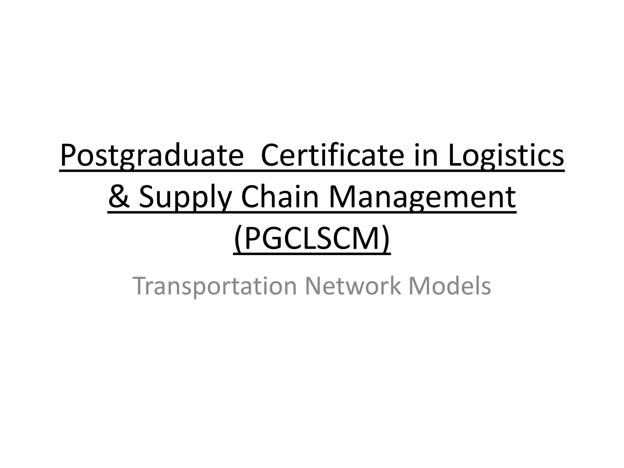


![Floyd-Warshall (All Pairs Shortest Path)
Initial Graph (Start State)
1. Dots represent arrow direction
2. Red edges are backward flows
3. 999 indicates no direct edge
4. Negative costs included 1 2 3 4 5
1
2
3
4
5
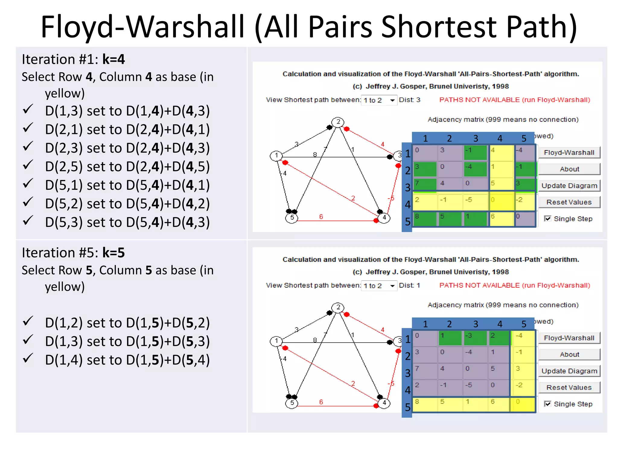
Iteration #1: k=1
Select Row 1, Column 1 as base (in
yellow)
For each cell D(i,j) (in purple) 1 2 3 4 5
Set D(i,j) = min[D(i,j) , D(i,k)+D(k,j)] 1
2
D(4,2) set to D(4,1)+D(1,2) 3
D(4,5) set to D(4,1)+D(1,5) 4
5
http://www.pms.ifi.lmu.de/lehre/compgeometry/Gosper/shortest_path/shortest_path.html#visualization](https://image.slidesharecdn.com/transportationnetworkmodels-120915012956-phpapp01/75/Transportation-network-models-30-2048.jpg)
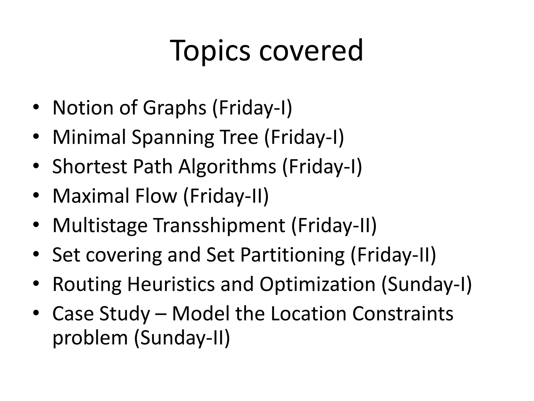
![Floyd-Warshall (All Pairs Shortest Path)
Iteration #2: k=2
Select Row 2, Column 2 as base (in
yellow)
For each cell D(i,j) (in purple)
1 2 3 4 5
Set D(i,j) = min[D(i,j) , D(i,k)+D(k,j)]
1
2
D(1,4) set to D(1,2)+D(2,4) 3
D(3,4) set to D(4,2)+D(2,3) 4
5
Iteration #3: k=3
Select Row 3, Column 3 as base (in
yellow)
For each cell D(i,j) (in purple) 1 2 3 4 5
Set D(i,j) = min[D(i,j) , D(i,k)+D(k,j)] 1
2
D(4,2) set to D(4,3)+D(3,2) 3
4
5](https://image.slidesharecdn.com/transportationnetworkmodels-120915012956-phpapp01/75/Transportation-network-models-31-2048.jpg)

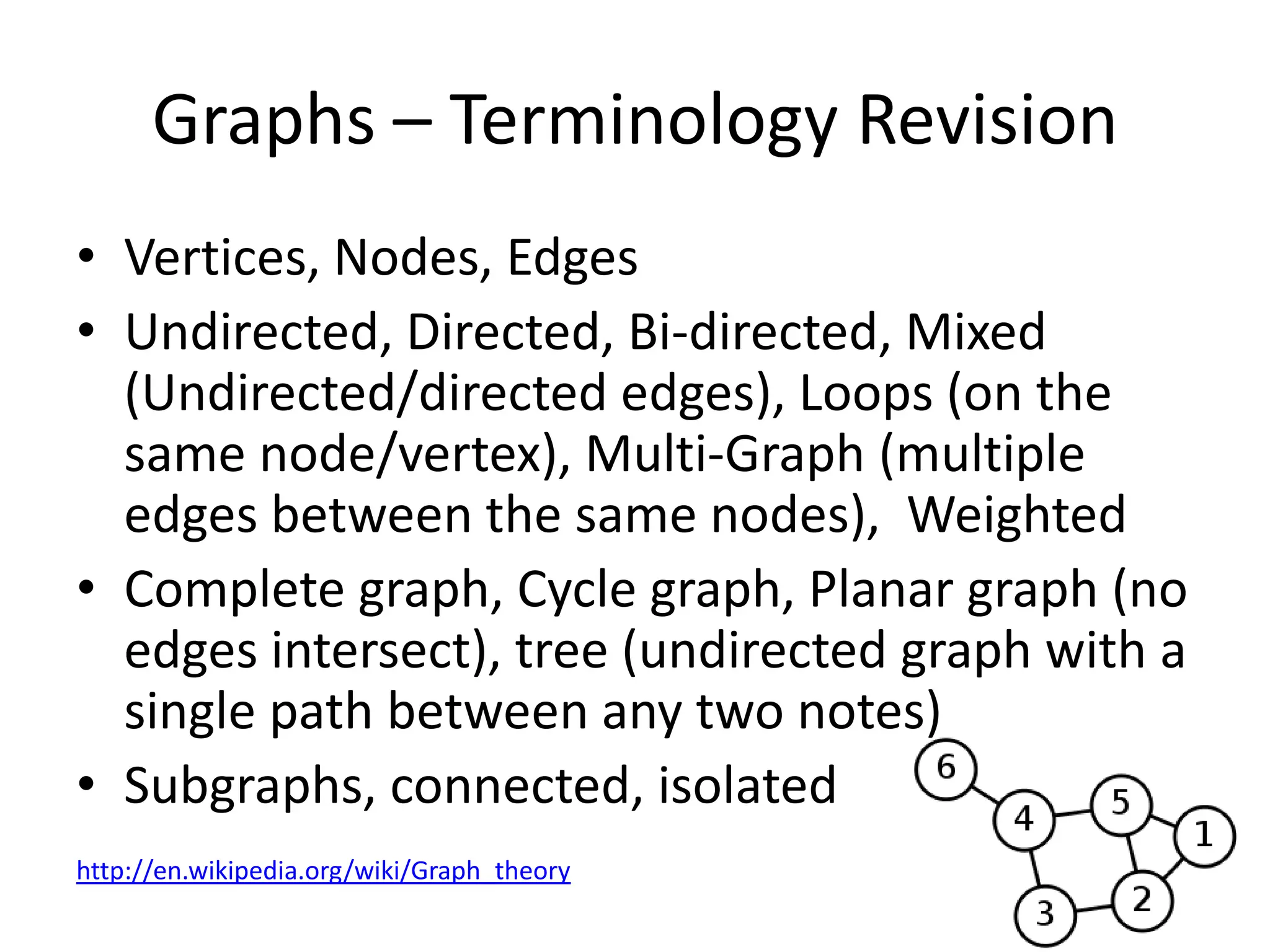
![Practical Application of Maximum Flow
• Tyson Foods, IBP Merger in 2001
– Combine Transportation Networks
– Optimize Fleet Carriers (Strategic), Residual Carriers (Contract and Spot
Carriers)
• Approach
– Mine trips data from previous 3 years
– Generate Aggregates (Min, Max, Avg) for each Lane/Start DOW/End DOW
– Run Flow problem iteratively for each start location and start day of week
[Modeled as a single node]
• Result (Cost optimization)
– Propose Routing Loops for Fleet Carriers
– Propose Residual Flow and suggested rates for Contract Negotiations](https://image.slidesharecdn.com/transportationnetworkmodels-120915012956-phpapp01/75/Transportation-network-models-35-2048.jpg)
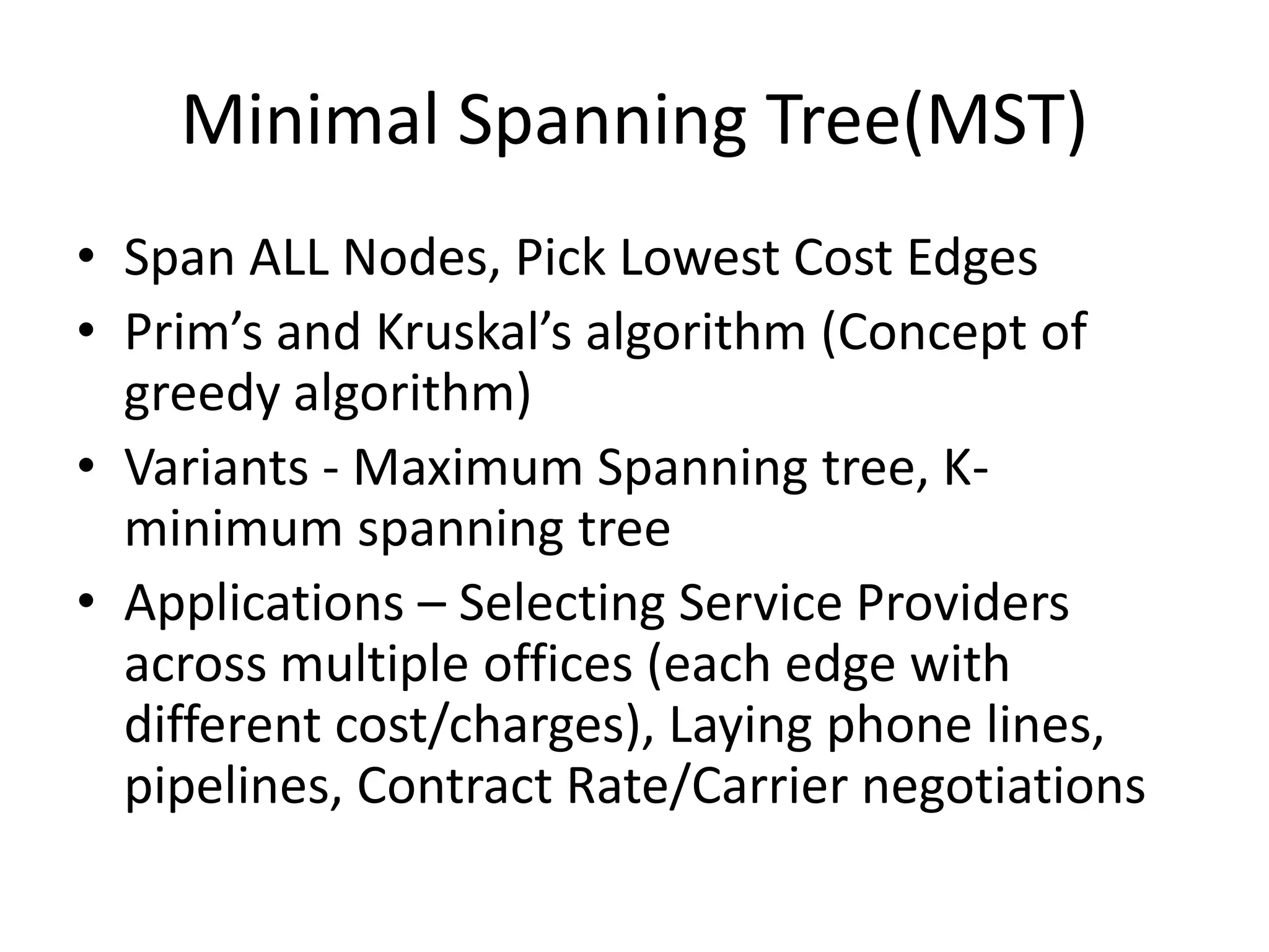
![Ford and Fulkerson Method
1. Find any path that has positive „forward‟ flow capacity
remaining
2. Compute f, the flow capacity on the bottleneck edge [This is
the most constricted flow in the chosen path]
3. Add f to the capacity in the forward direction of each edge in
the chosen path. Reduce f from the capacity in the reverse
direction of each edge in the chosen path
4. Repeat 1-3 until positive forward flow paths are found](https://image.slidesharecdn.com/transportationnetworkmodels-120915012956-phpapp01/75/Transportation-network-models-36-2048.jpg)
![Ford and Fulkerson Method
[Path A->D->E->G]
Flow on Bottleneck Arc [D->E]: 4
Reduce 4 in the forward direction edges
Add 4 in the reverse direction edges
Cumulative flow in the network = 4
[Path A->B->E->G]
Flow on Bottleneck Arc [B->E]: 3
Reduce 3 in the forward direction edges
Add 3 in the reverse direction edges
Cumulative flow in the network = 4+3](https://image.slidesharecdn.com/transportationnetworkmodels-120915012956-phpapp01/75/Transportation-network-models-37-2048.jpg)
![Ford and Fulkerson Method
[Path A->C->F->G]
Flow on Bottleneck Arc [A->C]: 4
Reduce 4 in the forward direction edges
Add 4 in the reverse direction edges
Cumulative flow in the network = 4+3+4
[Path A->D->F->G]
Flow on Bottleneck Arc [F->G]: 2
Reduce 2 in the forward direction edges
Add 2 in the reverse direction edges
Cumulative flow in the network = 4+3+4+2](https://image.slidesharecdn.com/transportationnetworkmodels-120915012956-phpapp01/75/Transportation-network-models-38-2048.jpg)
![Ford and Fulkerson Method
[Path A->D->F->E->G]
Flow on Bottleneck Arc [F->E]: 1
Reduce 1 in the forward direction edges
Add 1 in the reverse direction edges
Cumulative flow in the network = 14
(4+3+4+2+1).
There are no more positive flow paths
between A->G. The algorithm terminates.](https://image.slidesharecdn.com/transportationnetworkmodels-120915012956-phpapp01/75/Transportation-network-models-39-2048.jpg)
![Minimum Cut Problem
•Each ‘cut’ should detach all possible paths
from Source to Sink [A->G]
•‘cut value’ is the sum of flow capacities that
have been severed by the cut
Tit-bit: During Vietnam war, the infamous Ho Chi Minh trail(s) were modeled as
a network and ‘costs’ were associated with cutting the trail at various points.
The min cut then showed the set of trails that must be attacked to sever the flow of enemy
troops and supplies for the lowest cost operation.](https://image.slidesharecdn.com/transportationnetworkmodels-120915012956-phpapp01/75/Transportation-network-models-40-2048.jpg)
![Consolidation-Centered Heuristic
• Orders from the same origin and to the same destination can be combined to
Bundle one Trip/Shipment. Mode selection is made.
Orders
• Create Multi-Stop trips/shipments by consolidating within mode
[Courier, TruckLoad, LTL, Rail etc]
Consolidate • Assign Best Carrier, Rate
by Mode • Solve Vehicle Assignment problem for Truckload and LTL
• Disband under-utilized trips/shipment and evaluate alternate options to route
them or consolidate with other pre-existing trips
Disband • Assign Best Carrier Rate. Solve Vehicle Assignment problem
Underutilized](https://image.slidesharecdn.com/transportationnetworkmodels-120915012956-phpapp01/75/Transportation-network-models-46-2048.jpg)
![Objective Function
• Minimize total cost of solution
Minimize obj:
1000 x1 + 1234 x2 + 1343 x3 ….+ 2123 x10 + ….
[Cost of unique Trip and Start Time combination]
[All variables are made linear: 0 ≤ xi ≤ 1. Fractional results are converted to its
closest integer{0,1}. This makes the problem easier to solve. This is called Linear
Programming (LP) Relaxation.]
• Add Above (50,000 - Soft) and Below (3,000 - Soft) Target
Penalty variables
3000 x221 + 50000 x222 + 3000 x223 + 50000 x224 +……
* Integer programs are complicated to solve. Linear programs can be solved in polynomial time](https://image.slidesharecdn.com/transportationnetworkmodels-120915012956-phpapp01/75/Transportation-network-models-49-2048.jpg)
![Trip Constraints
• A trip can only start at one of its possible start times
Subject To
C1: x1 + x21 + x33 + x112 = 1 [x1, x21, x33 and x112 represent 4
different times trip can pickup at the location]
C2: x2 + x22 + x34 + x 113 = 1
…
…](https://image.slidesharecdn.com/transportationnetworkmodels-120915012956-phpapp01/75/Transportation-network-models-50-2048.jpg)
![Capacity Constraints
• Location can server two trips in each hour bucket
• Location can serve trips totaling 2000 KG in each hour
bucket
C101: x2 + x26 + x32 + x64 + x76 =2
[Each constraint corresponds to a specific 1-hour bucket. Each of the variables correspond to a trip at a particular pickup time
that falls in that one hour bucket. If that trip is selected, it contributes a trip count of 1 to the Bucket Capacity of 2 trips]
C102: 500x1 + 500x13 + 500x55 + 500x84 + 500x96 =2000
[Each constraint corresponds to a specific 1-hour bucket. Each of the variables correspond to a trip at a particular pickup time
that falls in that one hour bucket. If that trip is selected, it contributes 500 KG to the Bucket Capacity of 2000 KGS]
…
…
* Concept of Slack variables to accommodate lesser quantity than capacity](https://image.slidesharecdn.com/transportationnetworkmodels-120915012956-phpapp01/75/Transportation-network-models-51-2048.jpg)
![Balancing Constraints
• To create a balanced workload and prevent peaks. Helps
ramp-up and ramp-down labor resources
C201: x187 – x188 – x189 + x190 >=0
[The difference between adjacent time bucket assignments should be kept low].
Creates a pattern such as this ….
2.5
2
1.5
1 Series1
0.5
0
9 10 11 12 1 2 3 4 5](https://image.slidesharecdn.com/transportationnetworkmodels-120915012956-phpapp01/75/Transportation-network-models-52-2048.jpg)

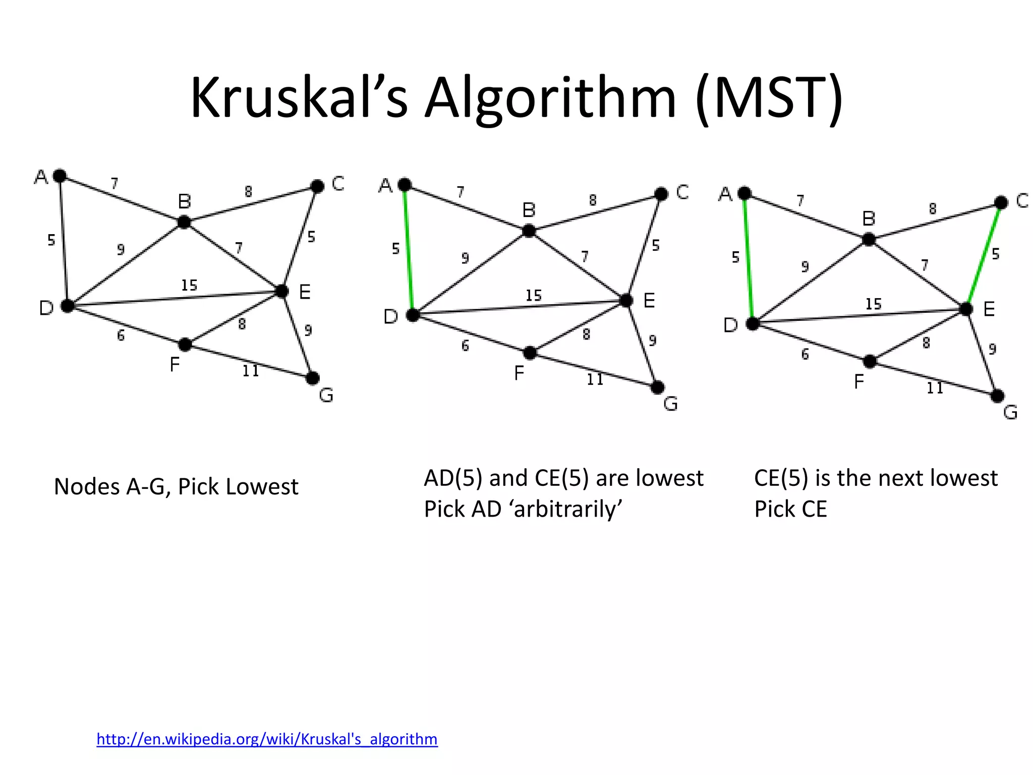
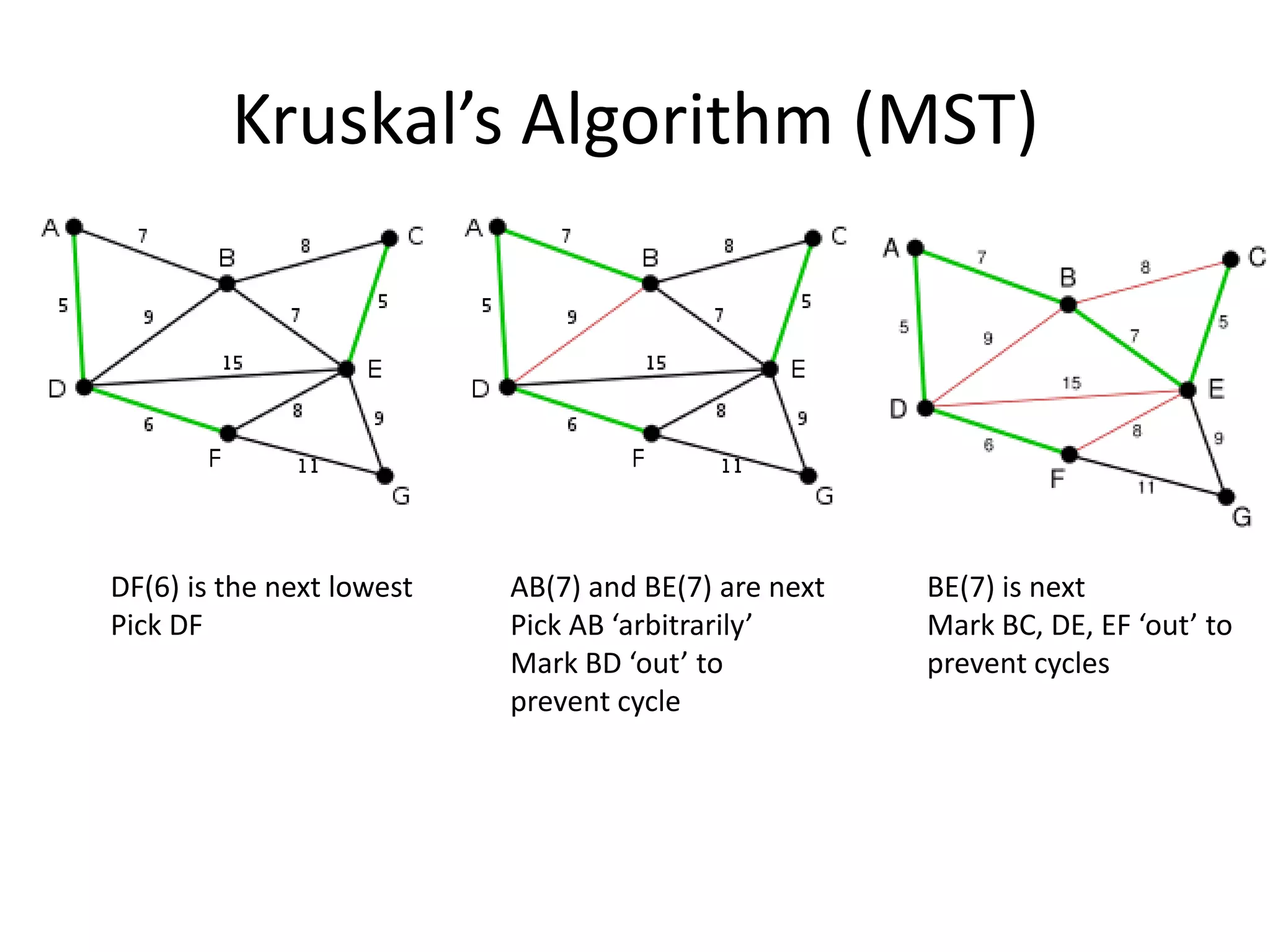
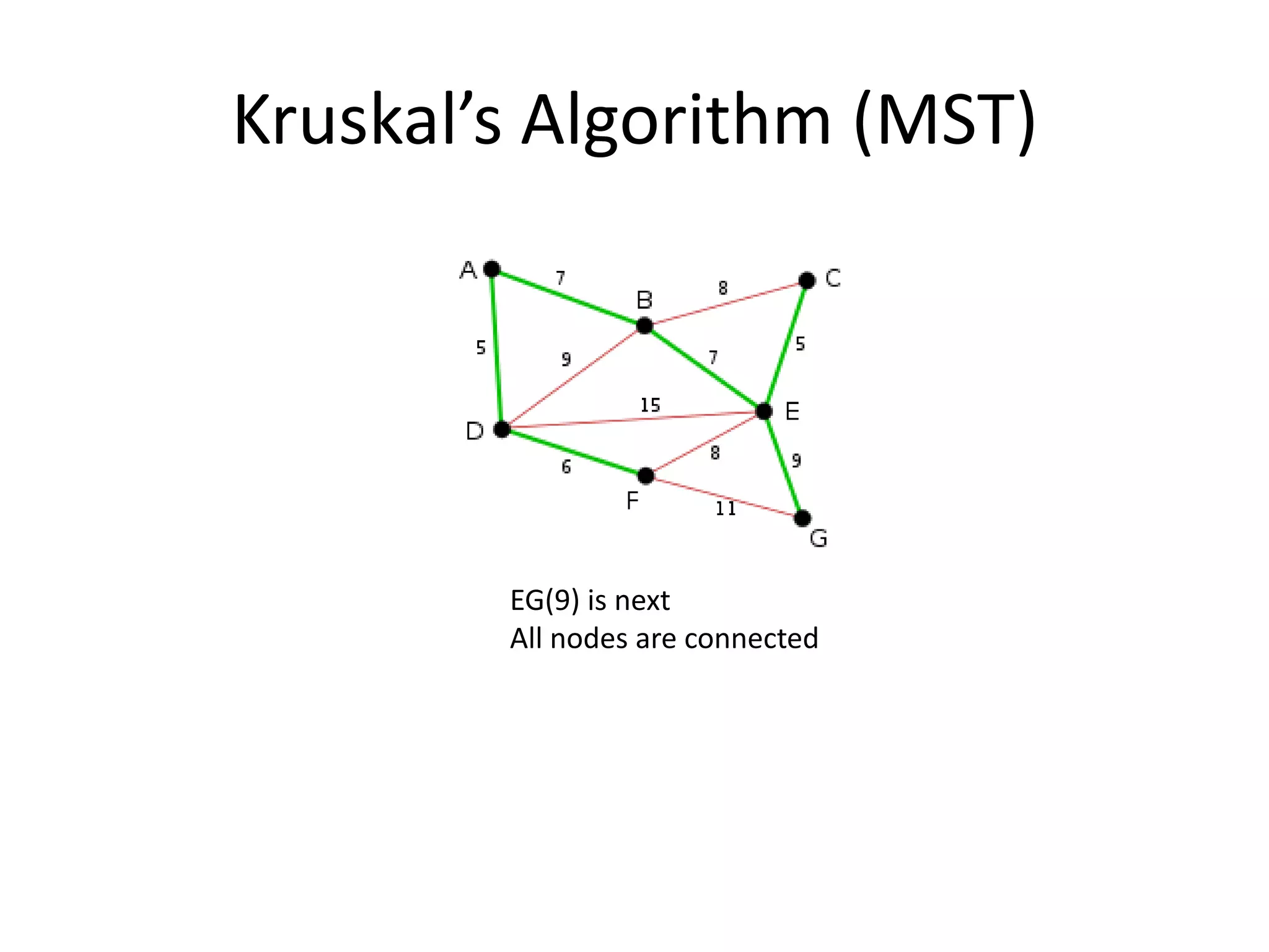
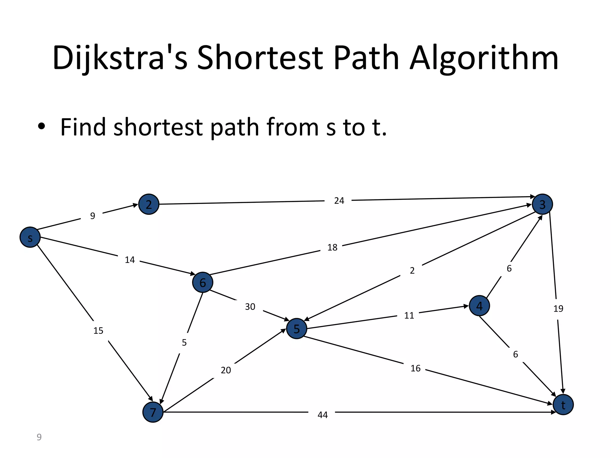
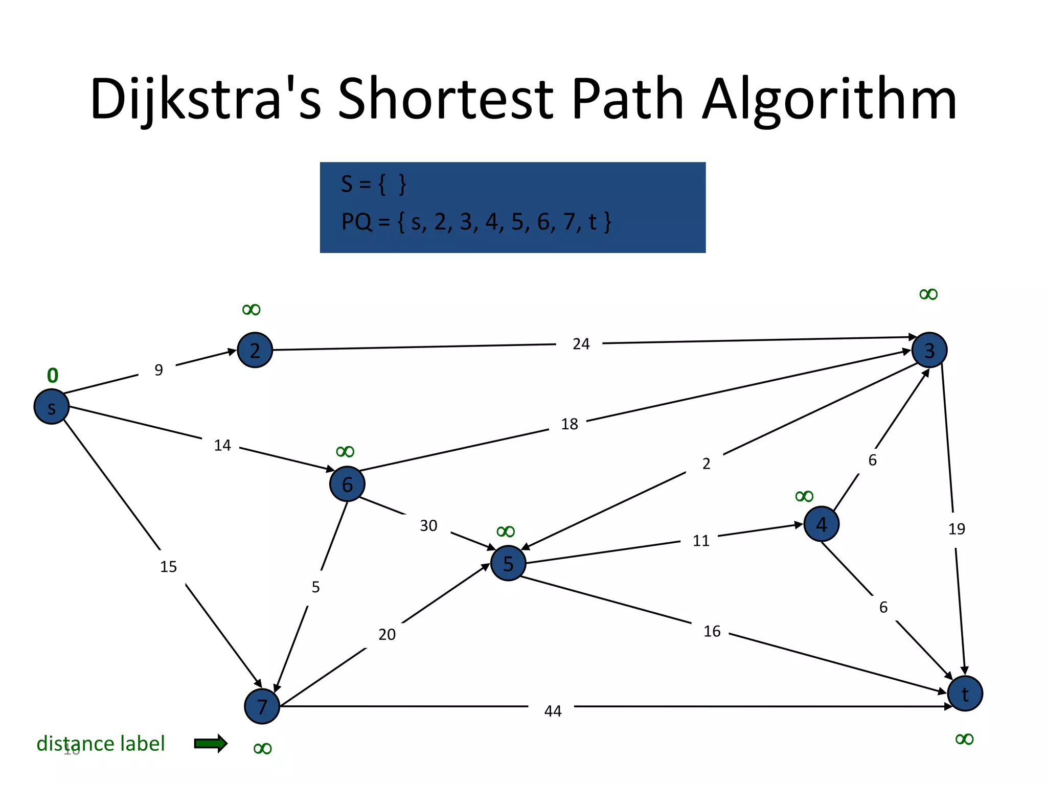
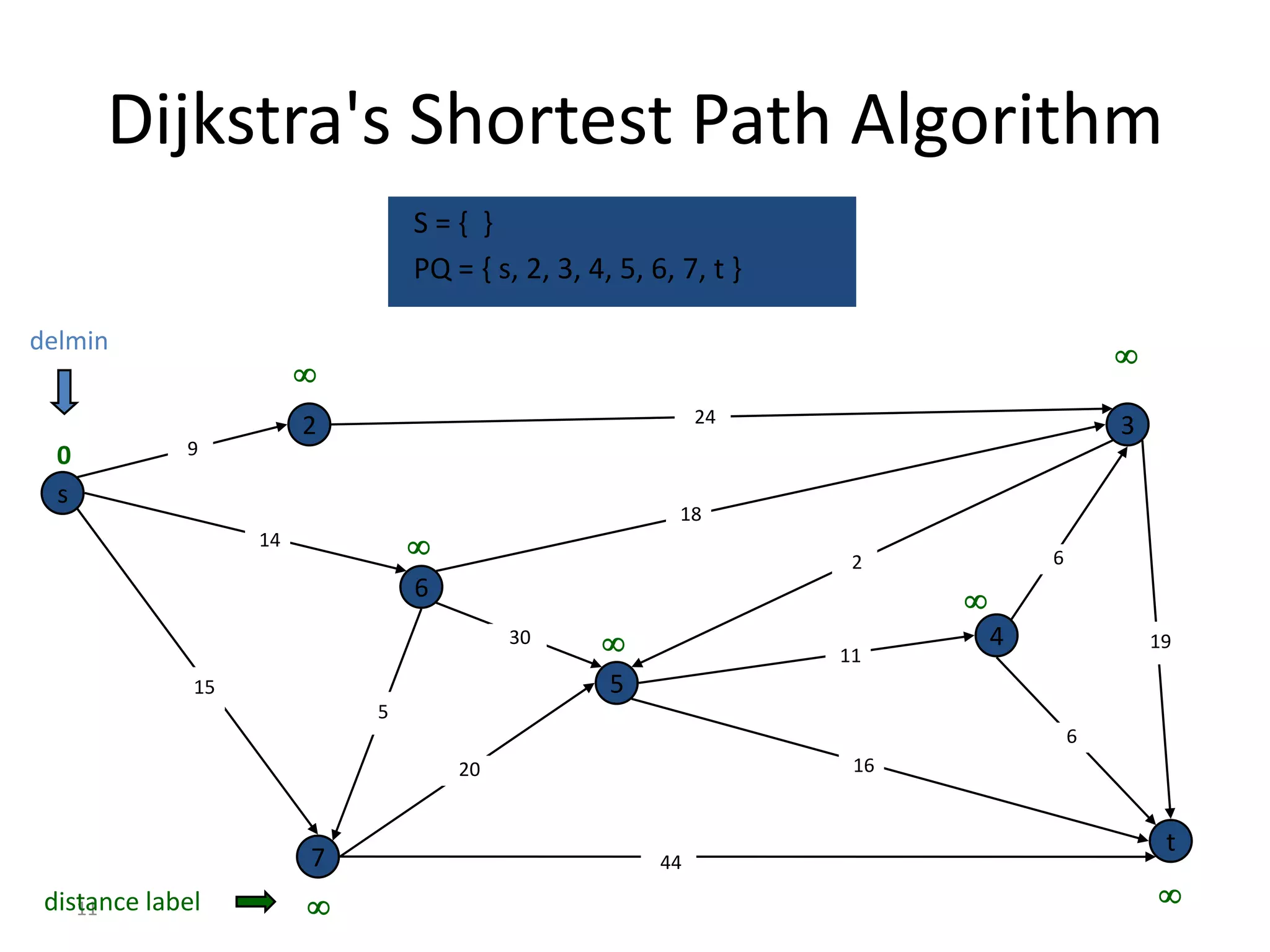
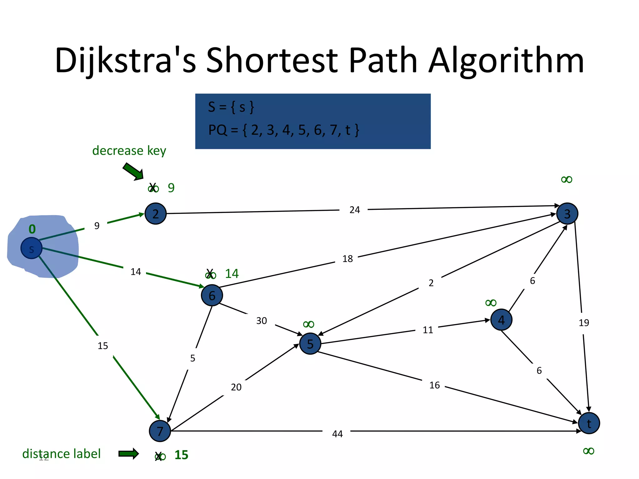
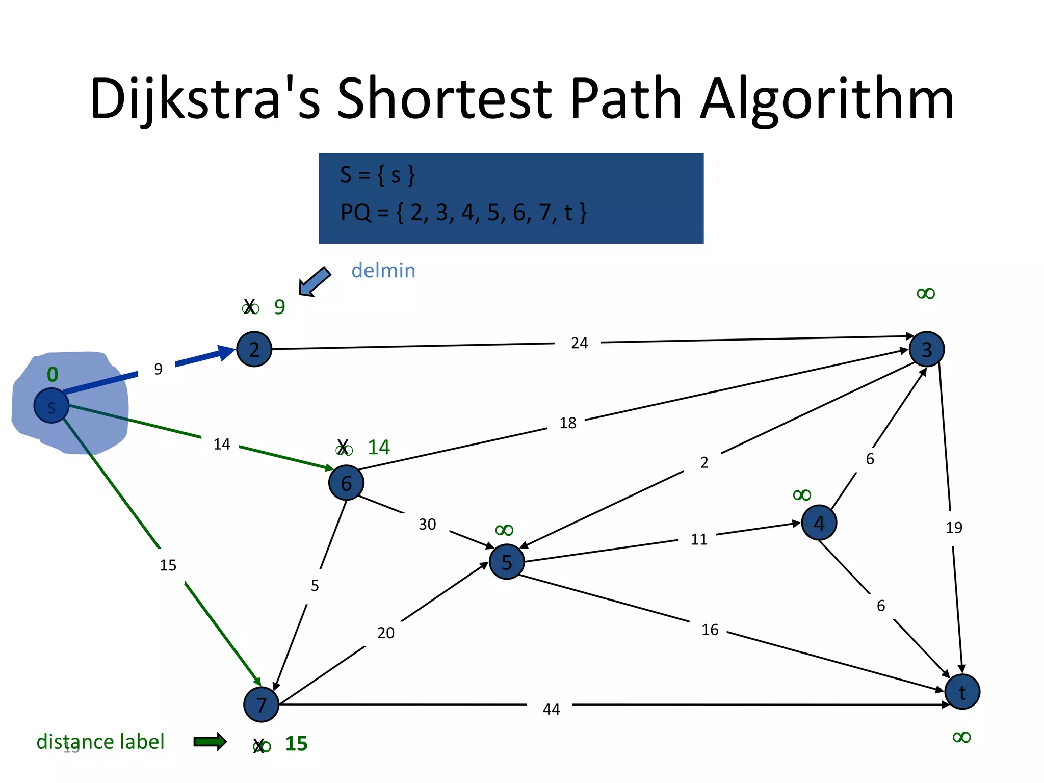
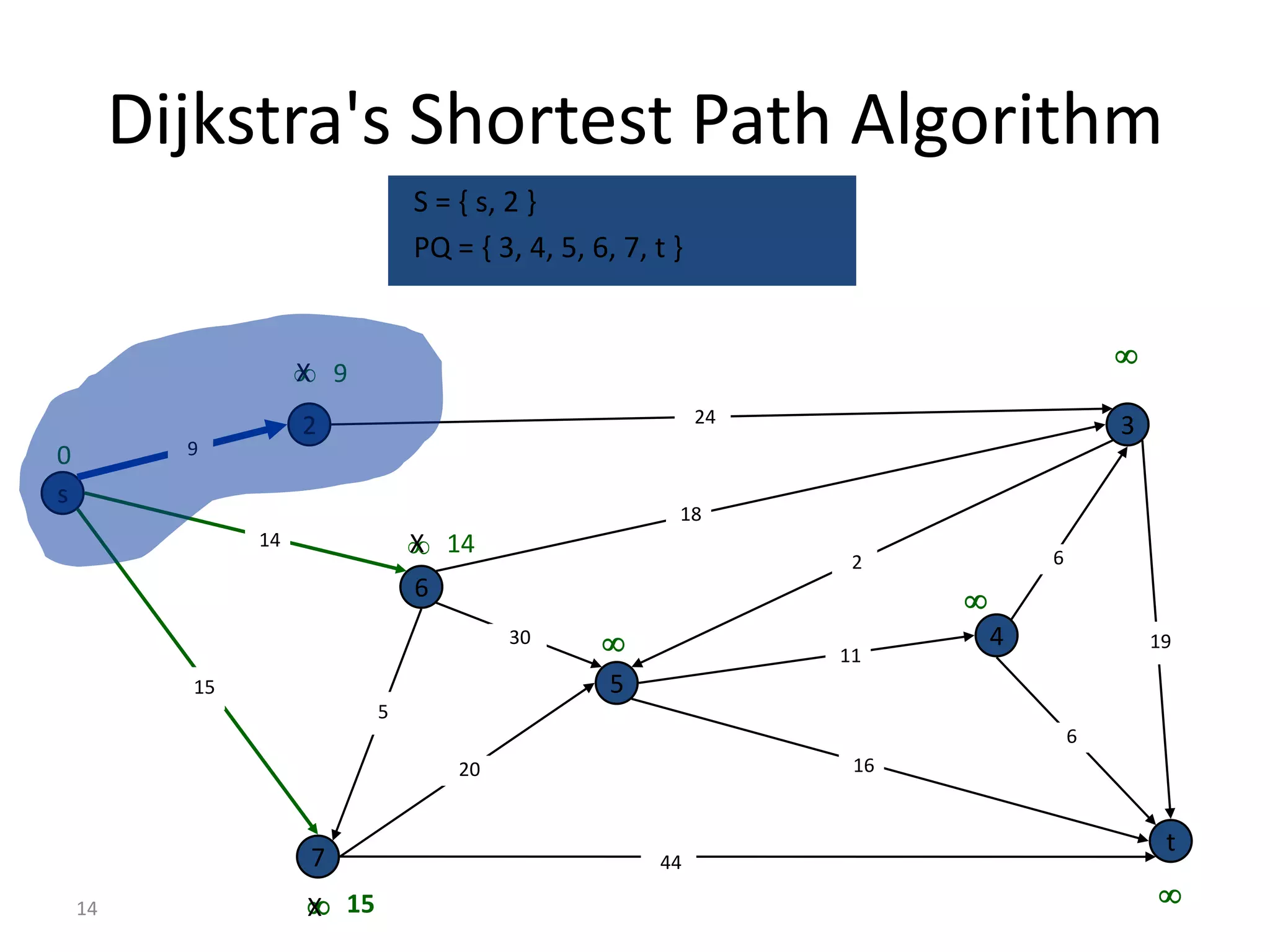
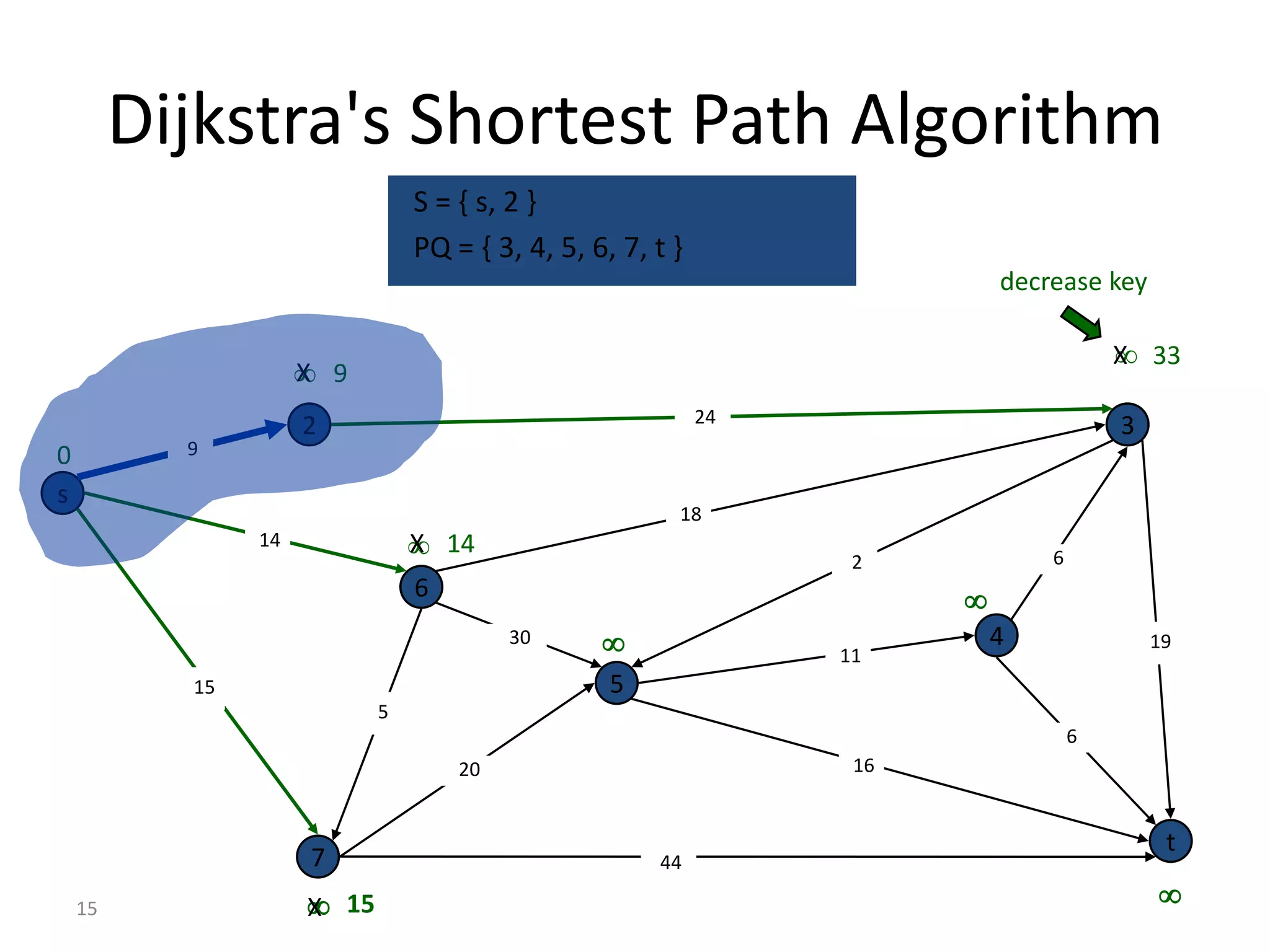
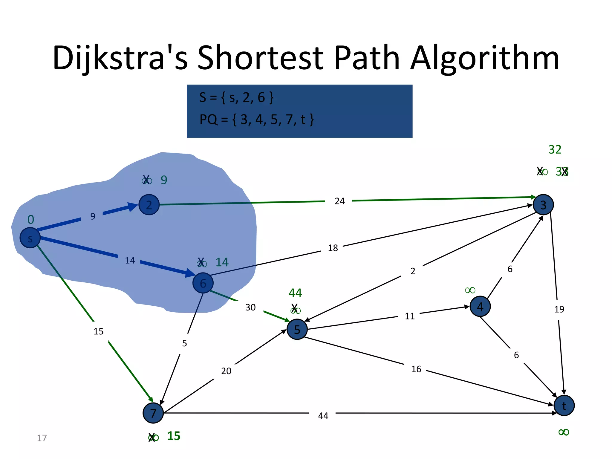
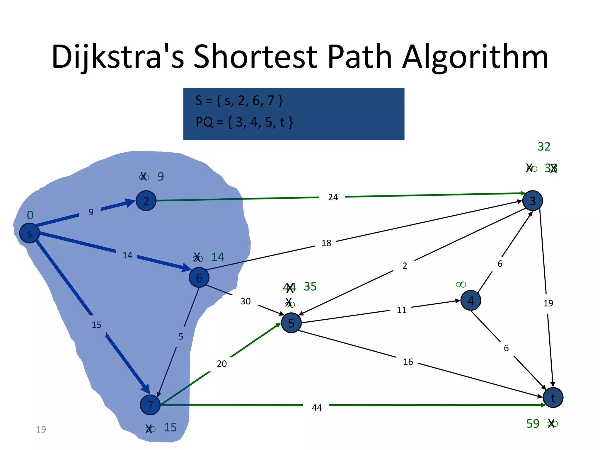
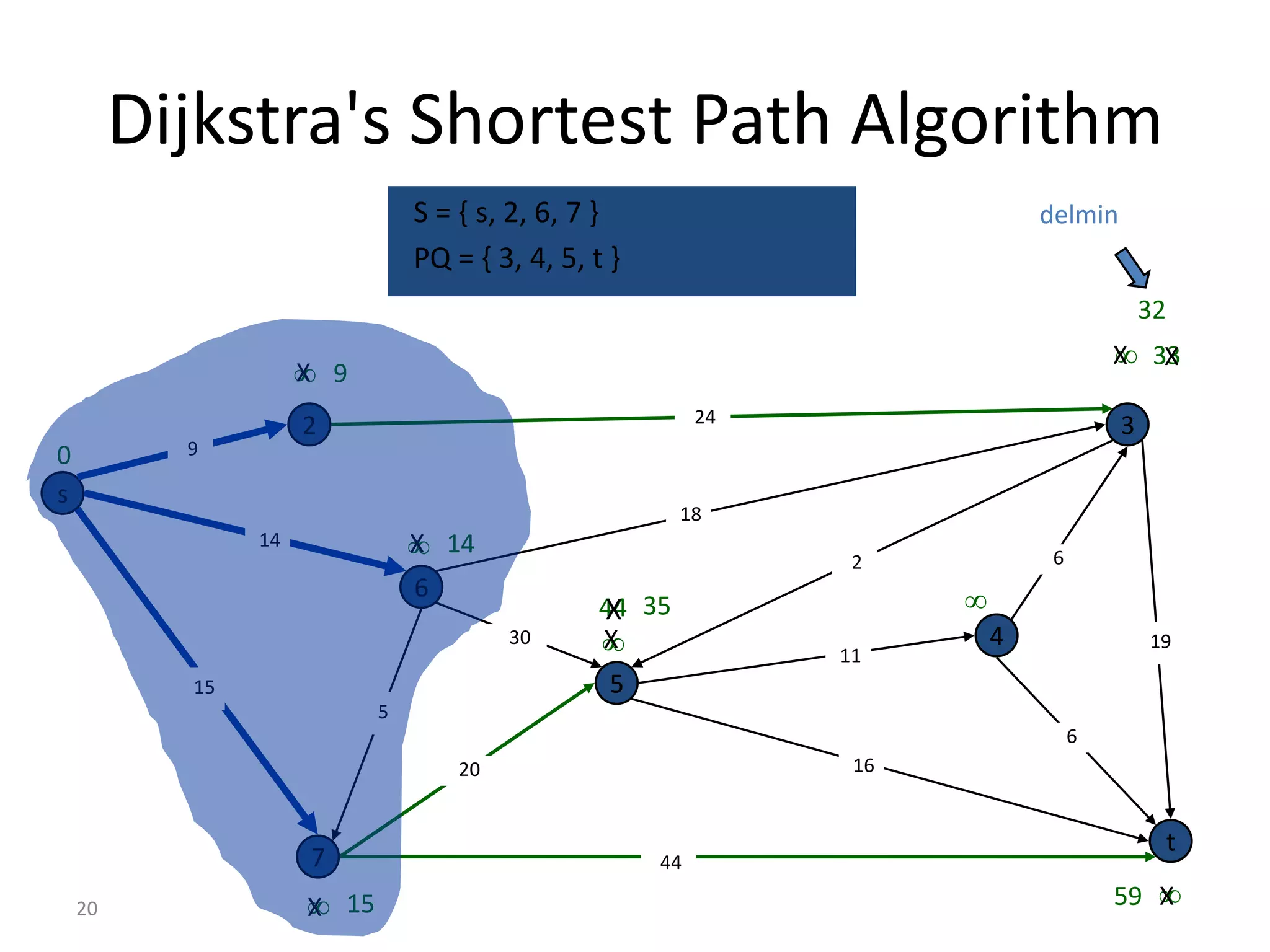
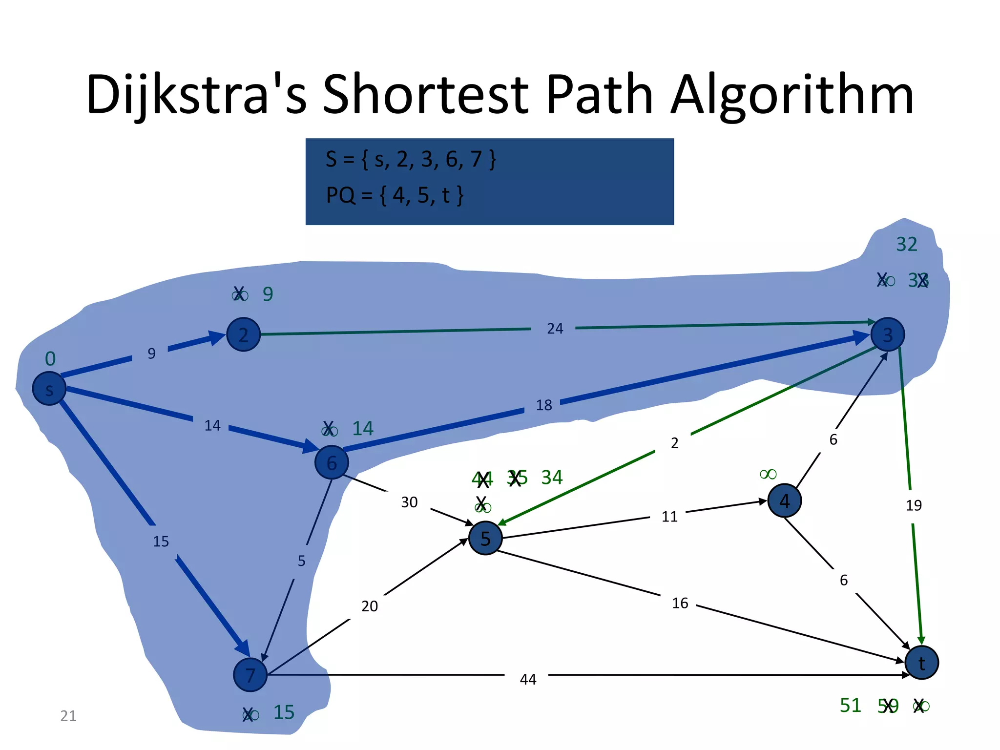
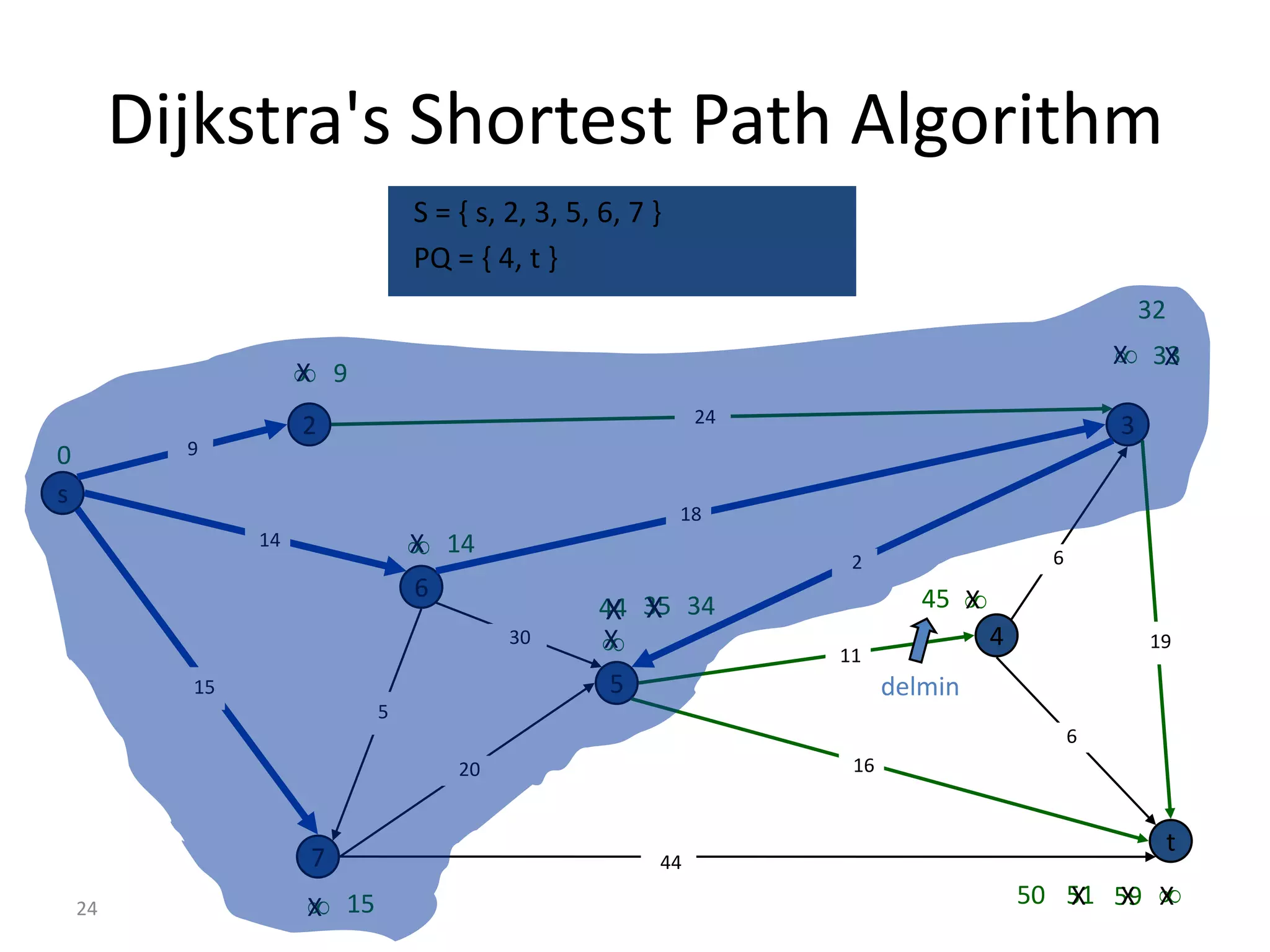
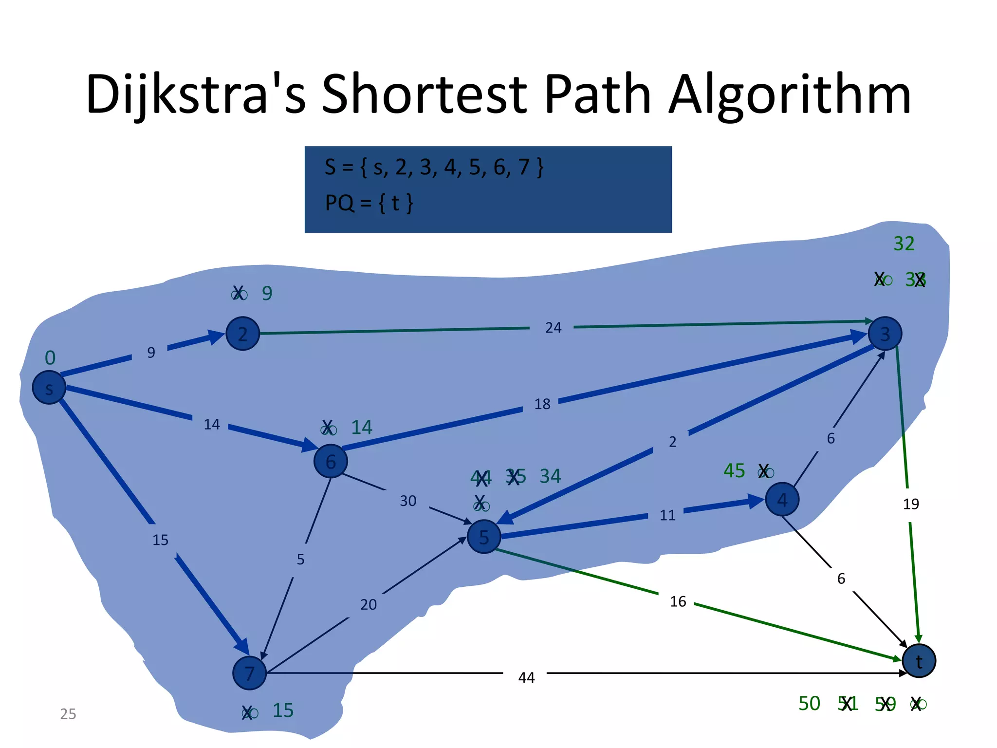
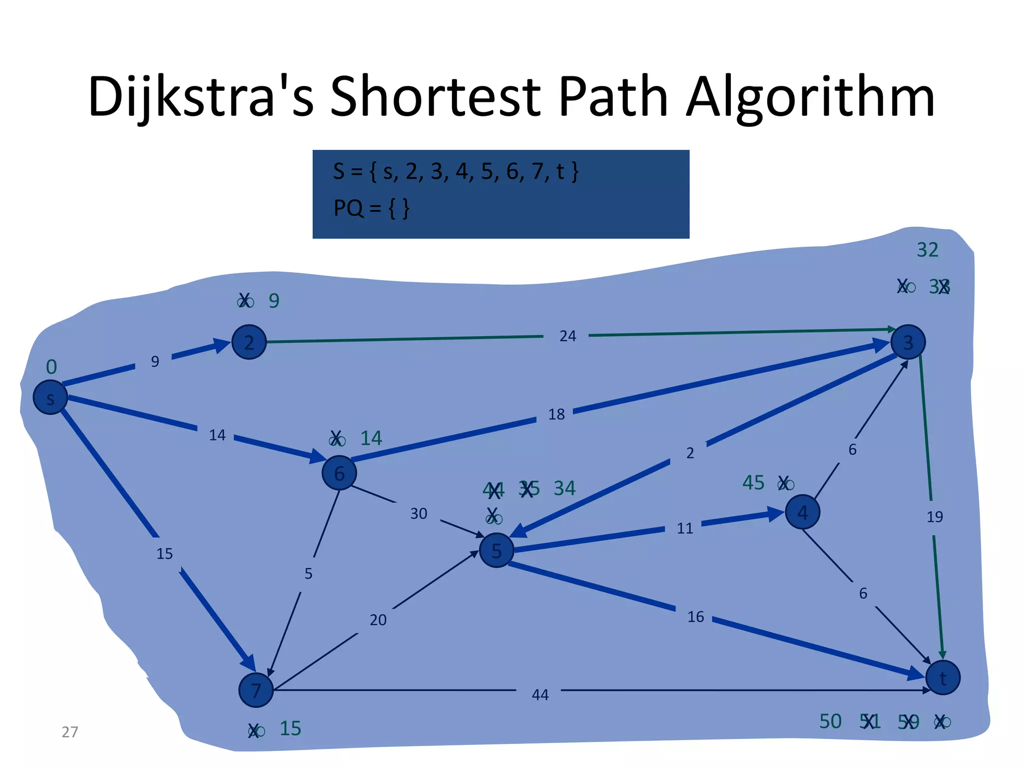
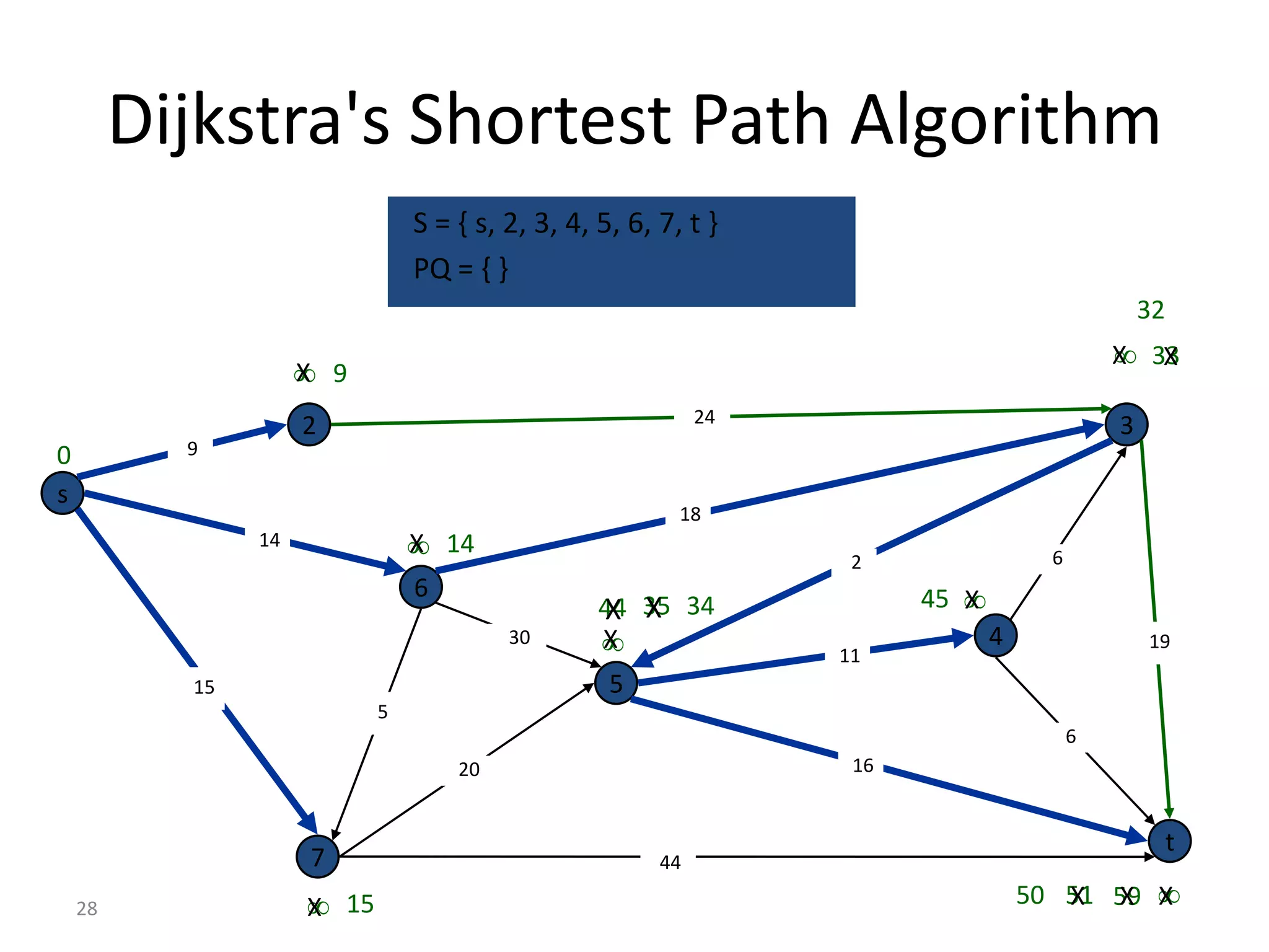
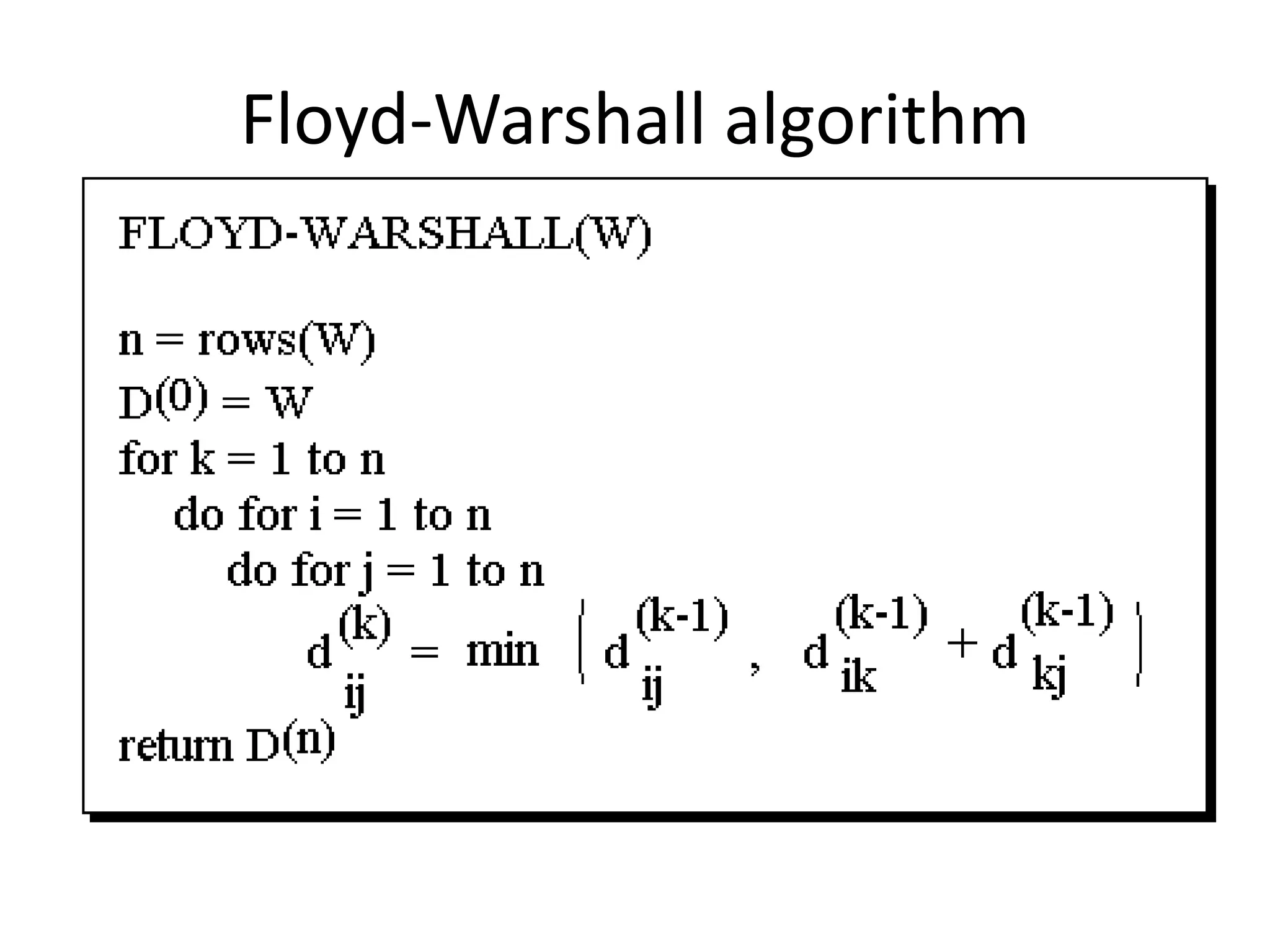
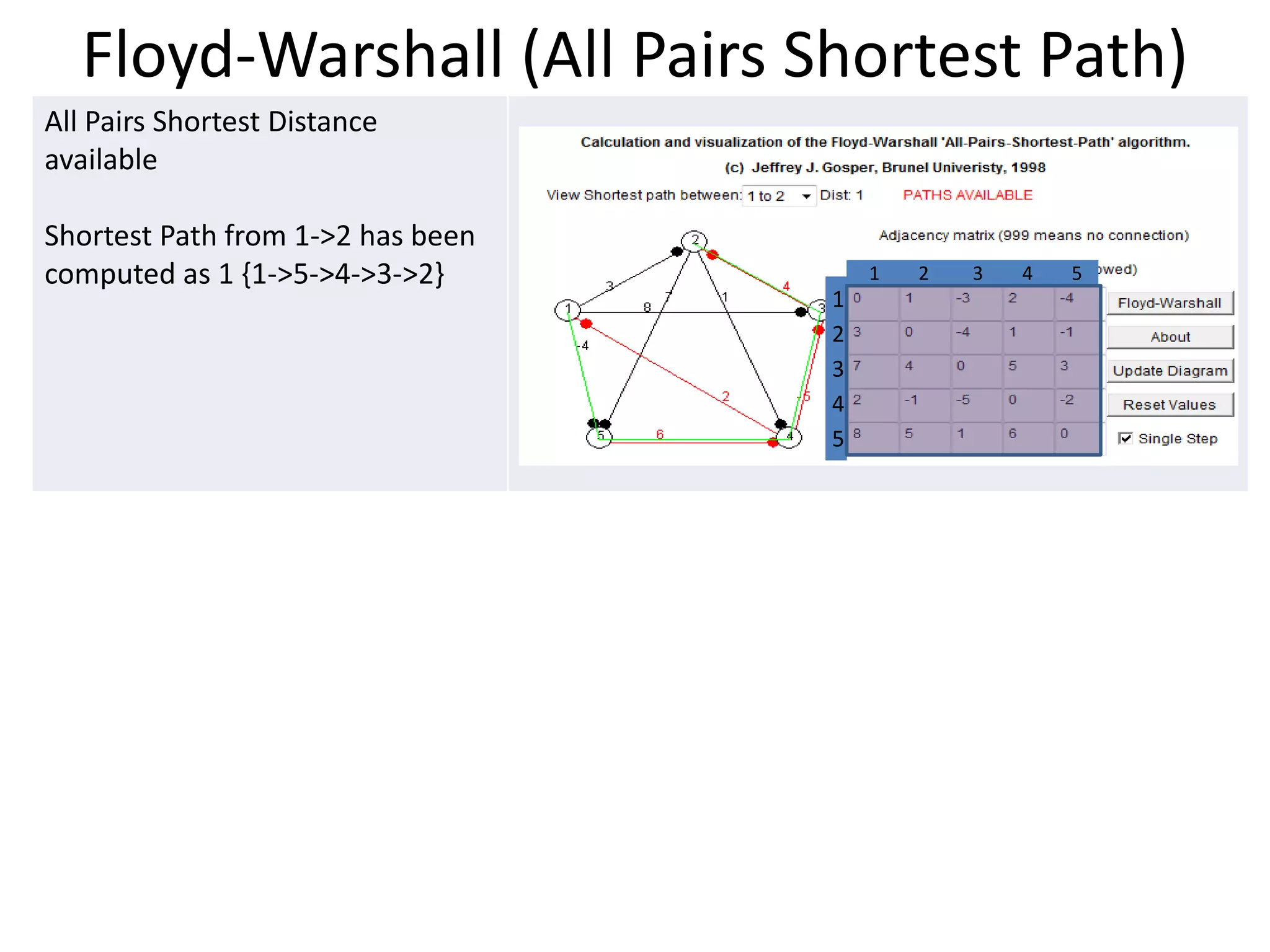
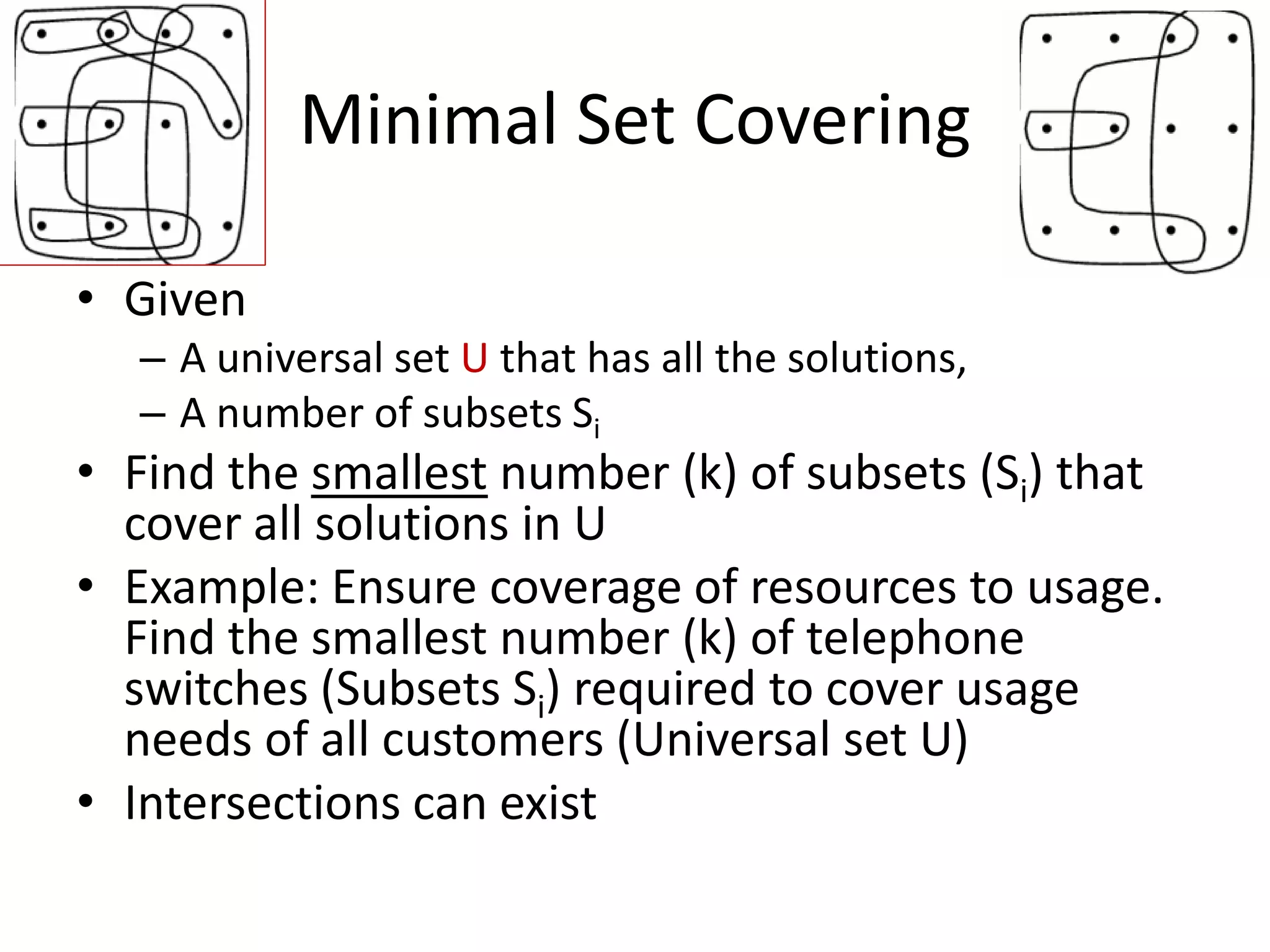
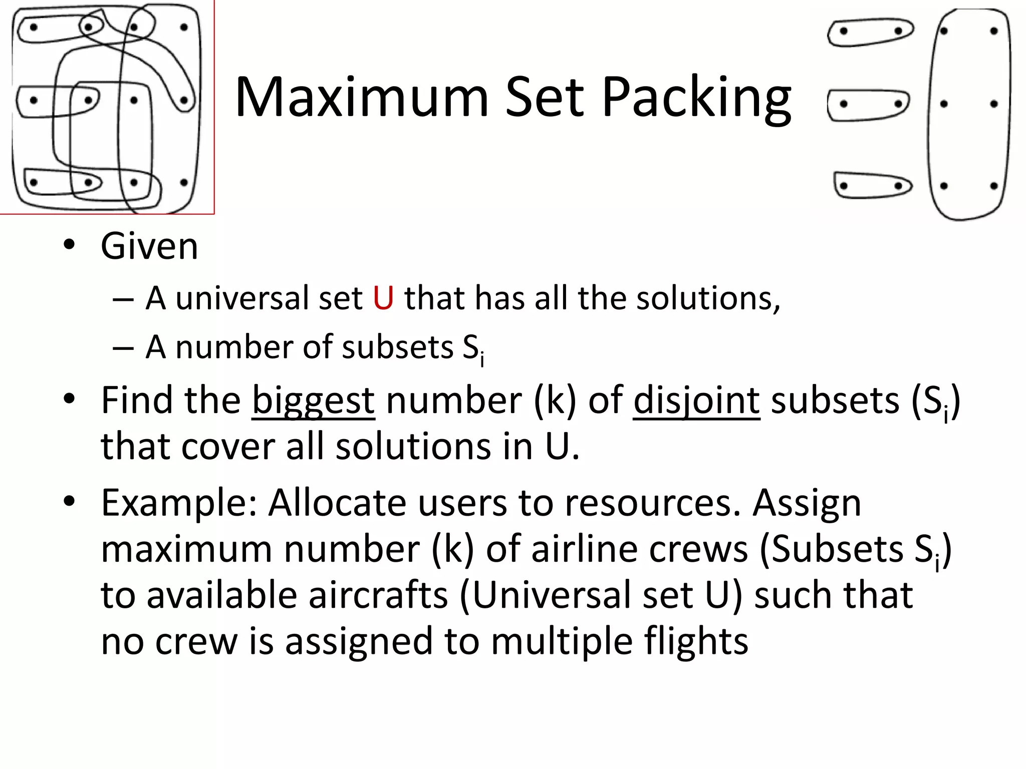
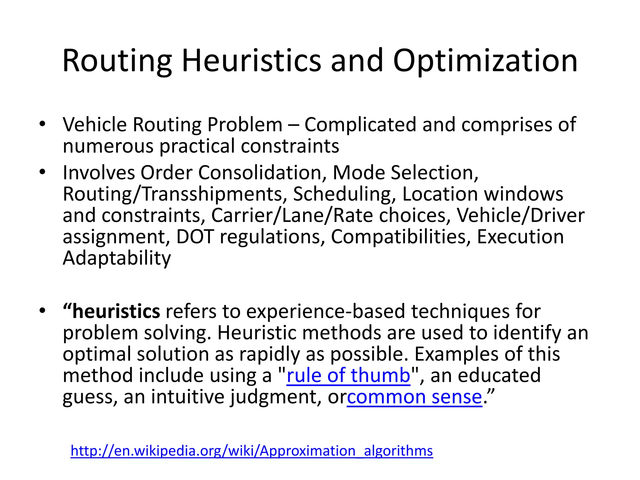
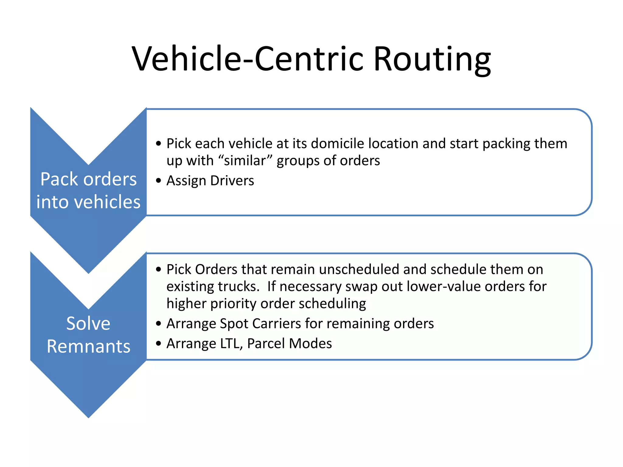
The document discusses various algorithms for solving transportation network models, including minimal spanning tree algorithms like Kruskal's and Prim's, shortest path algorithms like Dijkstra's and Floyd-Warshall, and maximal flow algorithms. It provides examples and step-by-step explanations of how Kruskal's and Dijkstra's algorithms work to find minimal spanning trees and shortest paths in graphs. Transportation network models have applications in logistics for routing vehicles and scheduling deliveries.


