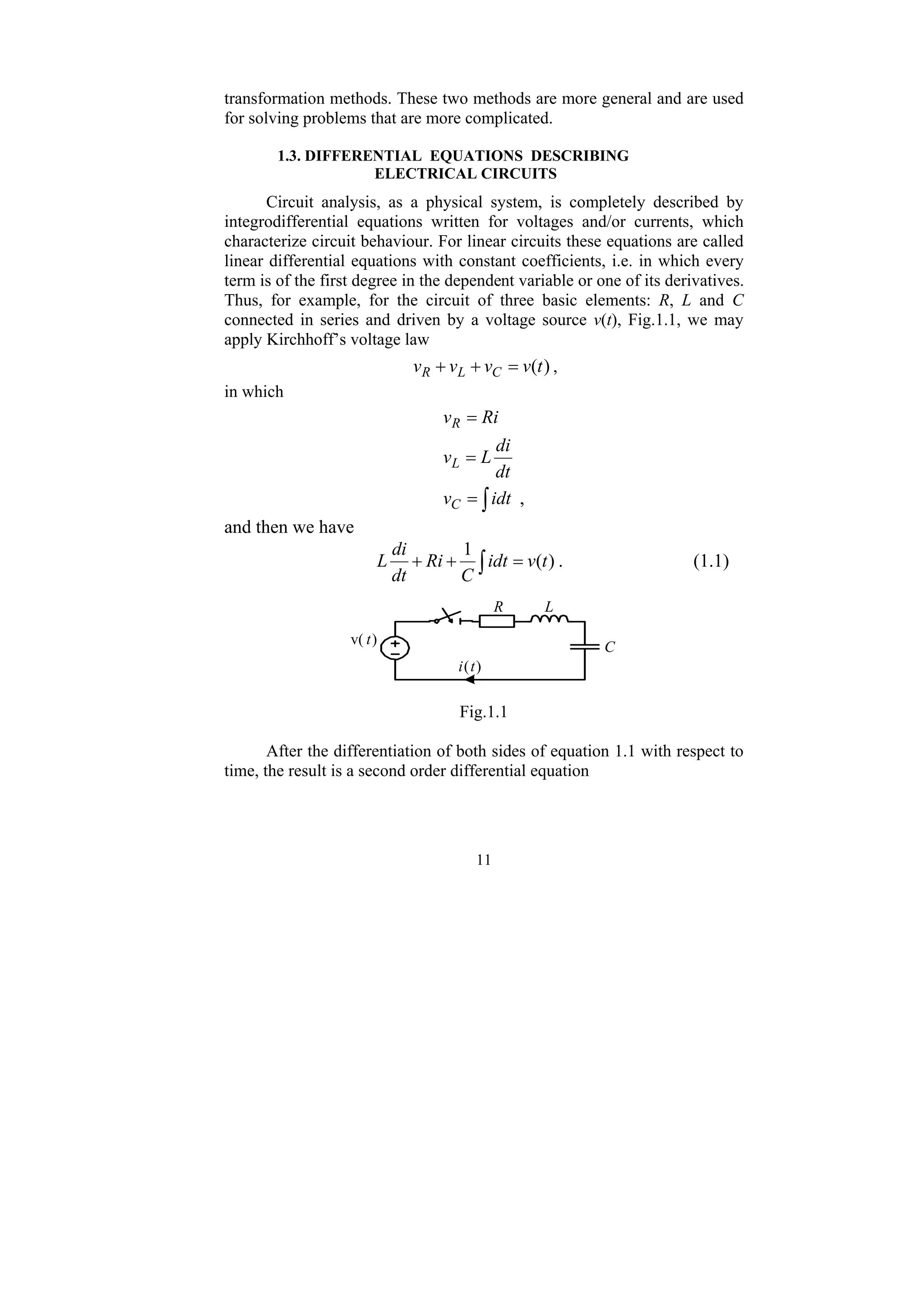
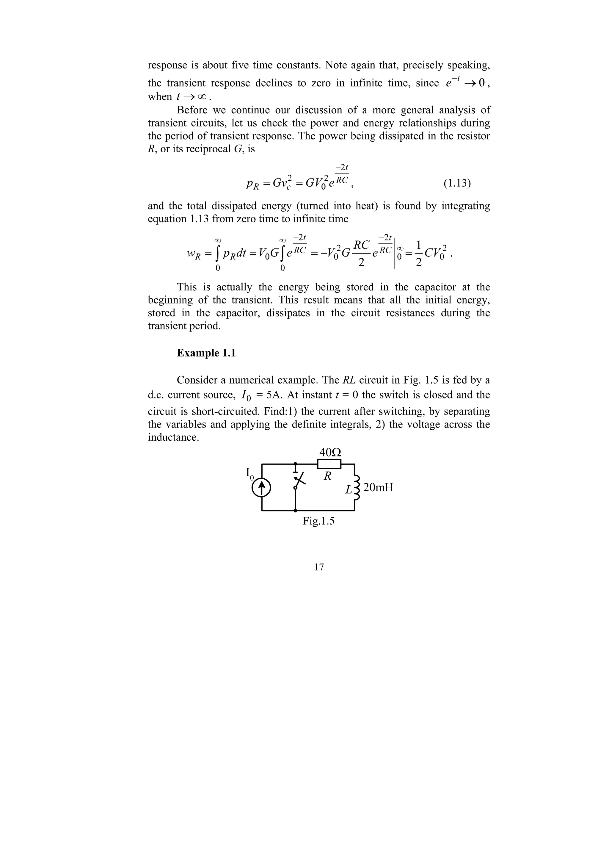
The document is a training book titled 'Transient Analysis of Electric Power Circuits by the Classical Method in the Examples,' aimed at advanced students in electrical engineering. It covers the theory and methods for analyzing transient responses in electrical circuits using classical techniques, providing solutions to typical problems for better understanding. The book serves as a link between introductory courses and more specialized texts, and is recommended for both students and professionals in the field.
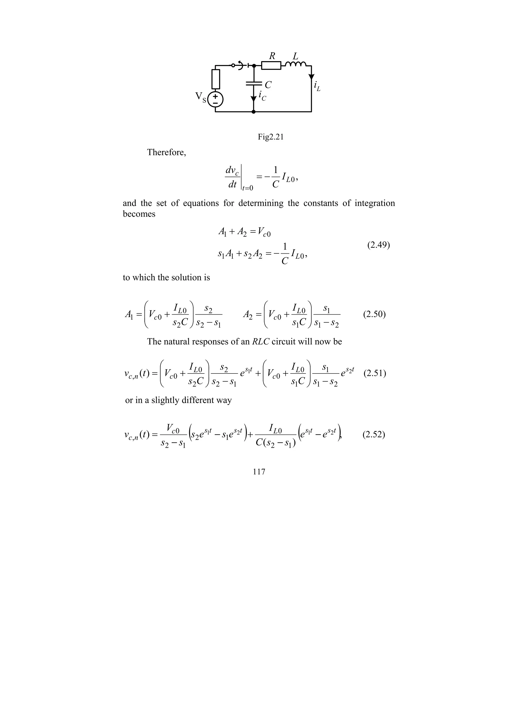
![16
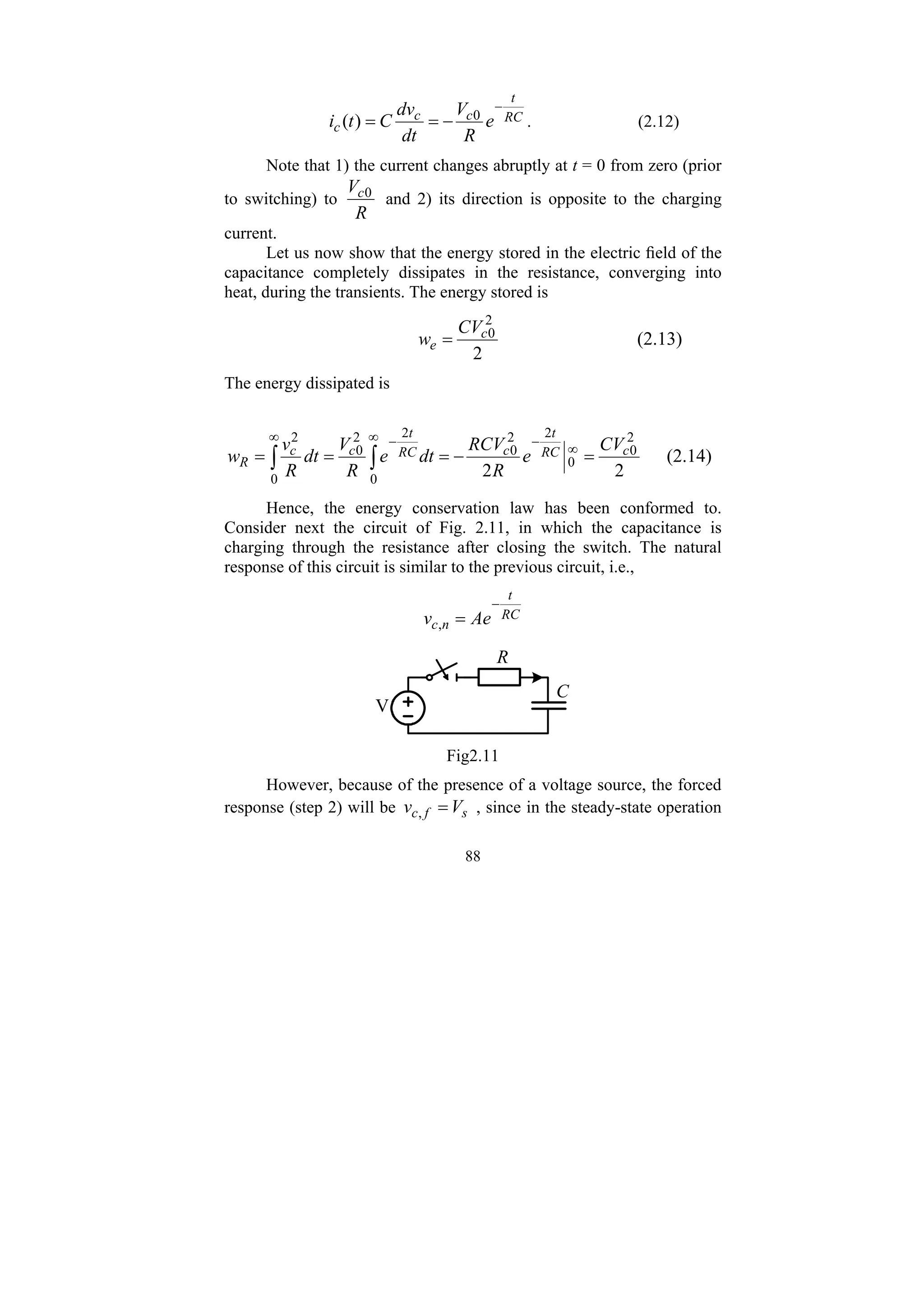
RC
t
c e
V
t
v
−
= 0
)
( (1.11)
We shall consider the nature of this response. At zero time, the
voltage is the assumed value 0
V and, as time increases, the voltage
decreases and approaches zero, following the physical rule that any
condenser shall finally be discharged and its final voltage therefore reduces
to zero.
Let us now find the time that would be required for the voltage to
drop to zero if it continued to drop linearly at its initial rate. This value of
time, usually designated by t, is called the time constant. The value of t can
be found with the derivative of )
(t
vc at zero time, which is proportional to
the angle c between the tangent to the voltage curve at t = 0, and the t-axis,
i.e.,
RC
V
e
V
dt
d
t
RC
t
0
0
0
−
=
⎟
⎟
⎠
⎞
⎜
⎜
⎝
⎛
=
−
or
τ = RC
and equation 1.11 might be written in the form
τ
0
)
(
t
c e
V
t
v
−
= (1.12)
The units of the time constant are seconds ([τ] = [R][C] = Ω·F), so
that the exponent t/RC is dimensionless, as it is supposed to be.
Another interpretation of the time constant is obtained from the fact
that in the time interval of one time constant the voltage drops relatively to
its initial value, to the reciprocal of e; indeed, at t = τ we have
%)
8
,
36
(
368
,
0
1
0
=
= −
e
V
vc
. At the end of the 5t interval the voltage is less
than one percent of its initial value. Thus, it is usual to presume that in the
time interval of three to five time constants, the transient response declines
to zero or, in other words, we may say that the duration of the transient](https://image.slidesharecdn.com/transientanalysisofelectricalpowercircuit-240923113814-129745da/75/Transient-Analysis-of-Electrical-Power-Circuit-pdf-16-2048.jpg)
![53
The energy stored in the magnetic field of two inductances prior
to switching is
2
)
0
(
2
)
0
(
)
0
(
2
2
2
2
1
1 −
−
− +
= L
L
m
i
L
i
L
w (1.50a)
and after switching
2
)
0
(
)
(
)
0
(
2
2
1 +
+
+
= L
m
i
L
L
w (1.50b)
Then the amount of energy dissipated in the first stage of the
transients, i.e., in circuit resistances and in the arc, with equations 1.50a
and 1.50b will be
[ ]2
2
1
2
1
2
1
)
0
(
)
0
(
2
1
)
0
(
)
0
( −
−
+
− −
+
=
−
=
Δ L
L
m
m
m i
i
L
L
L
L
w
w
w (1.51)
For the circuit under consideration the above equation 1.51
becomes
2
0
2
1
2
1
2
1
I
L
L
L
L
wm
+
=
Δ (1.52)
It is interesting to note that this expression is similar to formula
1.43 for a capacitance circuit. Let us now consider a numerical example.
Example 1.7
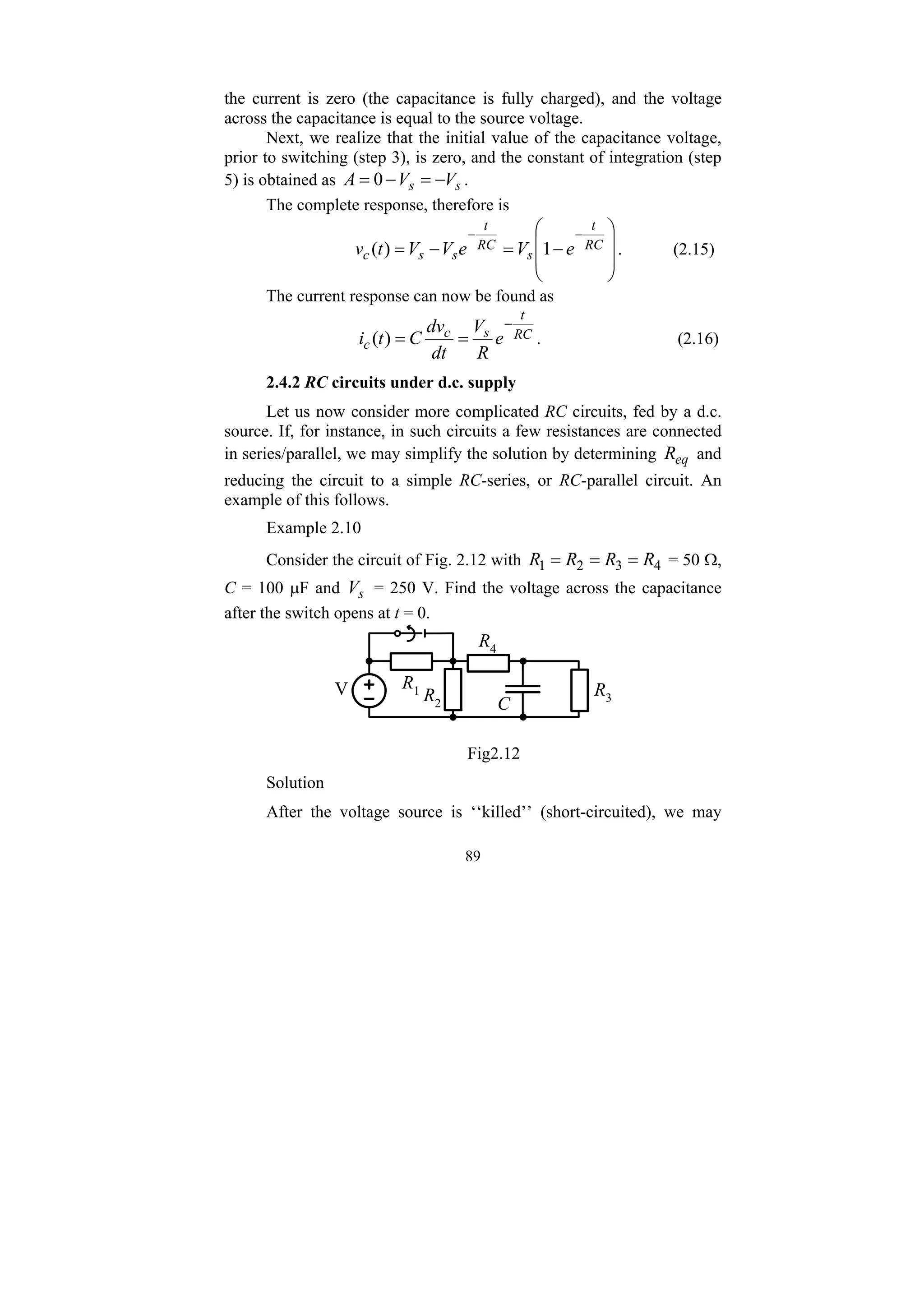
In the circuit in Fig. 1.20(a) the switch opens at instant t = 0. Find
the initial current )
0
( +
i in the second stage of the transient response
and the energy dissipated in the first stage if the parameters are:
Ω
= 50
1
R , Ω
= 40
2
R , mH
L 160
1 = , mH
L 40
2 = , in
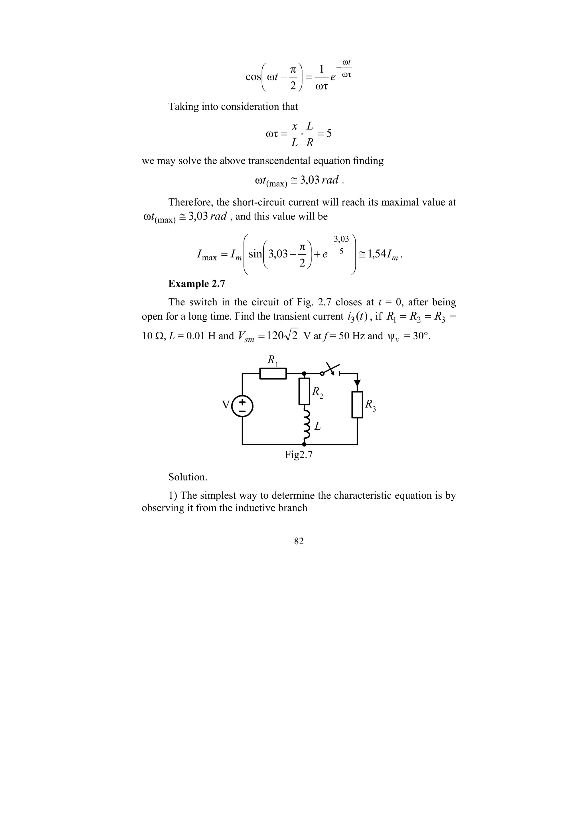
V = 200 V.](https://image.slidesharecdn.com/transientanalysisofelectricalpowercircuit-240923113814-129745da/75/Transient-Analysis-of-Electrical-Power-Circuit-pdf-53-2048.jpg)
![54
L2 L1
R1
R2
Uin
L2
L1
R1
R2
i(0+
)
b
a
Fig1.20
Solution.
The values of the two currents in circuit (a) are
A
R
V
i in
L 4
)
0
(
1
1 =
=
−
and
A
R
V
i in
L 5
)
0
(
2
2 =
=
−
Thus, the initial value of the current in circuit (b), in accordance
with equation 1.49, is
A
L
L
i
L
i
L
i L
L
L 2
,
2
40
160
5
40
4
160
)
0
(
)
0
(
)
0
(
2
1
2
2
1
1
+
⋅
−
⋅
=
+
−
= −
−
+ .
Note that for the calculation of the initial current )
0
( +
i in circuit
(b), we took into consideration that the current )
0
(
2 −
L
i is negative
since its direction is opposite to the direction of )
0
( +
i , which has been
chosen as the positive direction. The dissipation of energy, in
accordance with equation 1.51, is
[ ] J
L
L
i
i
L
L
w L
L
m 3
,
1
)
(
2
)
0
(
)
0
(
2
1
2
2
1
2
1
≅
+
−
=
Δ −
−
.
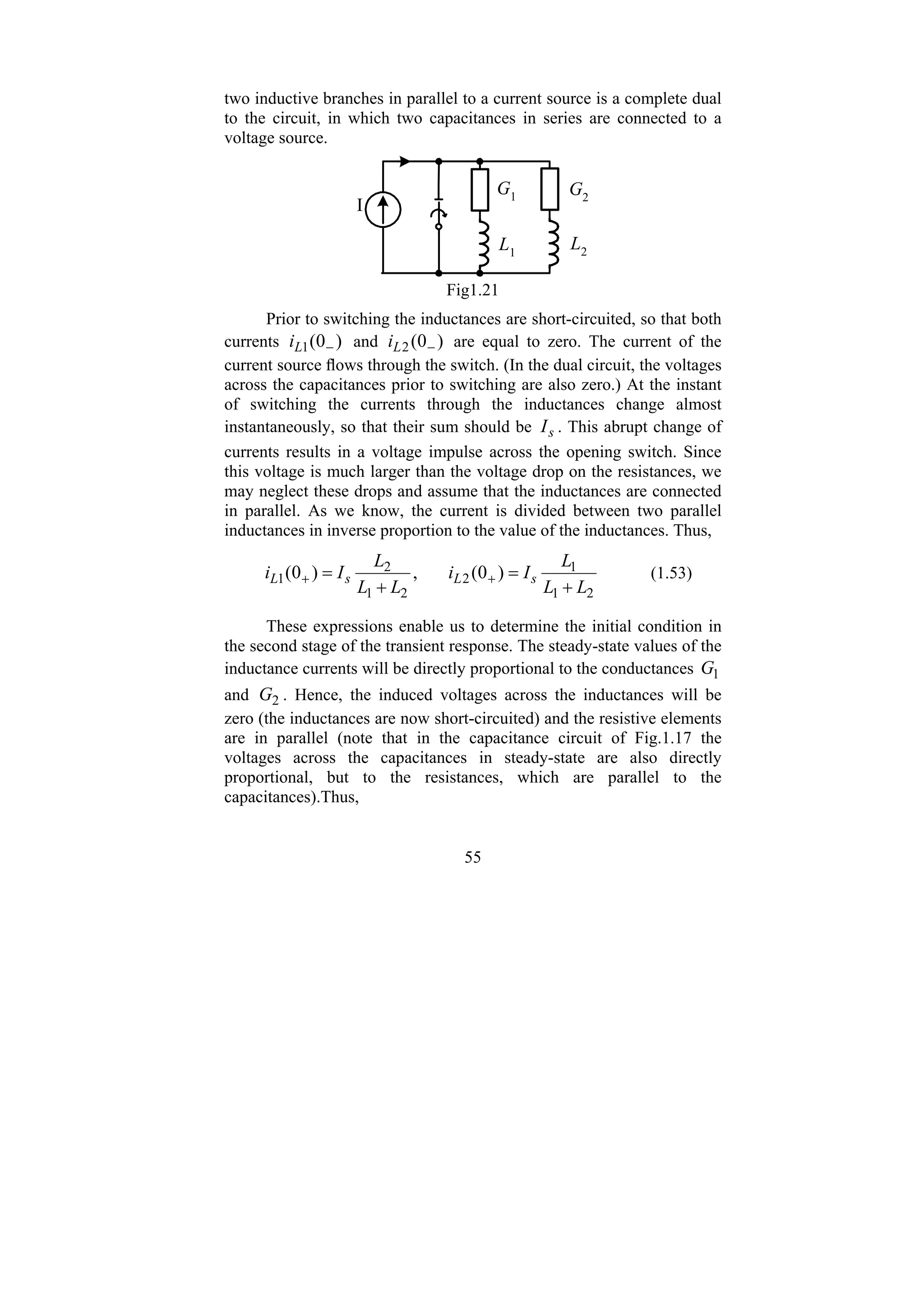
As a final example, consider the circuit in Fig. 1.21. This circuit of](https://image.slidesharecdn.com/transientanalysisofelectricalpowercircuit-240923113814-129745da/75/Transient-Analysis-of-Electrical-Power-Circuit-pdf-54-2048.jpg)
![65
st
f
f e
i
i
t
i
t
i )]
0
(
)
0
(
[
)
(
)
( −
+
= + (2.2b)
Keeping the above-classified rules in mind, we shall analyze (in
the following sections) the transient behaviour of different circuits.
2.3. FIRST ORDER RL CIRCUITS
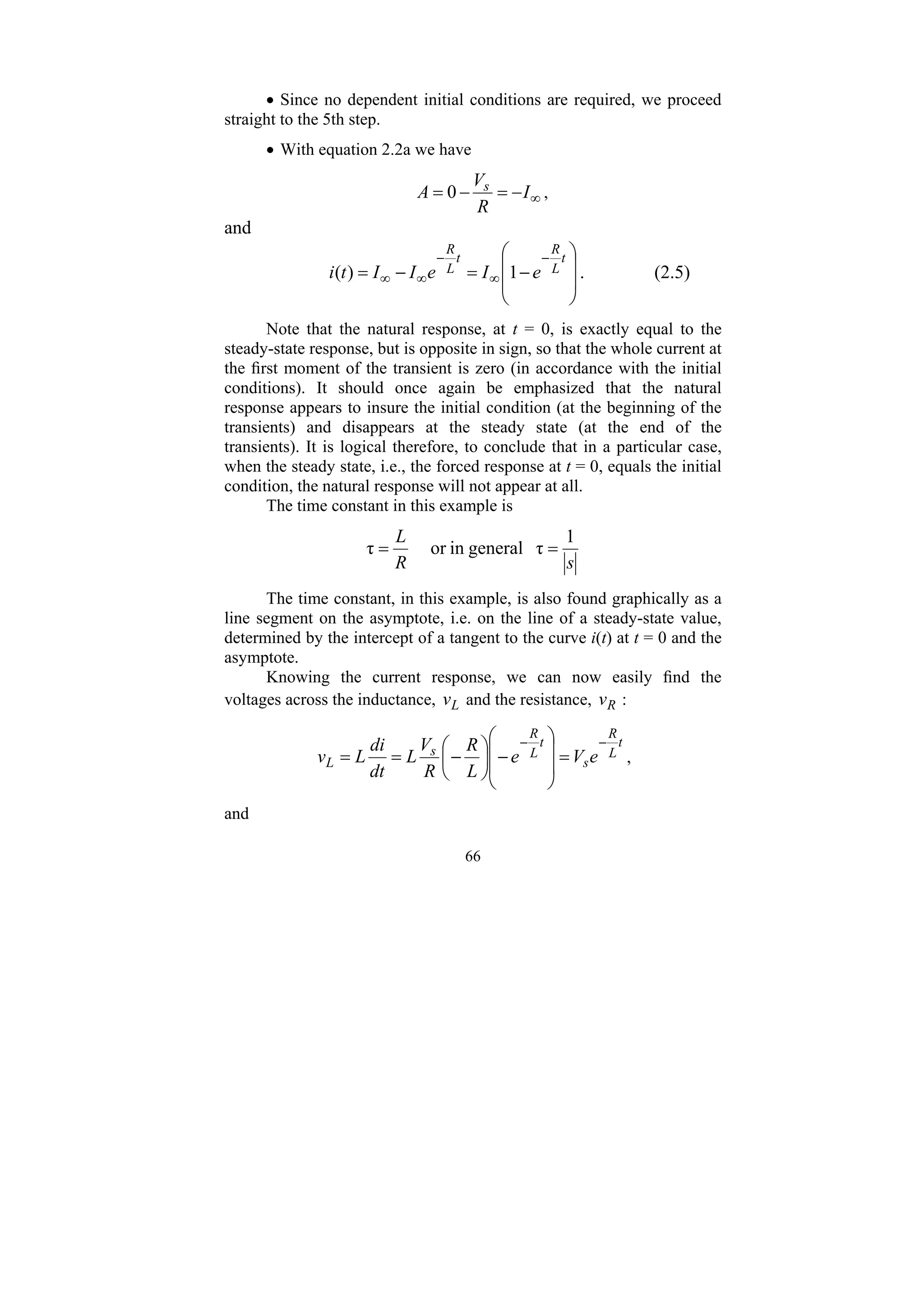
2.3.1. RL circuits under d.c. supply
Let us start with a simple RL series circuit, which is connected to
a d.c. voltage source, to illustrate how to determine its complete
response by using the 5-step solution method. This circuit has been
previously analyzed (in its short-circuiting behaviour) by applying a
mathematical approach.
• Determining the input impedance and equating it to zero yields
0
)
( =
+
= sL
R
s
Zin (2.3a)
The root of these equations is
L
R
s −
= (2.3b)
Thus, the natural response will be
t
L
R
n Ae
t
i
−
=
)
( (2.3c)
• The forced response, i.e. the steady-state current (after the
switch is closed, at ∞
→
t , the inductance is equivalent to a short
circuit) will be
∞
=
= I
R
V
t
i s
f )
( (2.4)
• Because the current through the inductance, prior to closing the
switch, was zero, the independent initial condition is
0
)
0
(
)
0
( =
= −
+ L
L i
i](https://image.slidesharecdn.com/transientanalysisofelectricalpowercircuit-240923113814-129745da/75/Transient-Analysis-of-Electrical-Power-Circuit-pdf-65-2048.jpg)
![94
2) By inspection of the circuit in Fig. 2.14, in its steady-state
operation (after the switch had been open for a long time), we may
conclude that the only current flowing through resistance 2
R is the
current of the current source, i.e., s
f I
i =
,
2 = 1 A.
3) In order to determine the independent initial condition, i.e. the
capacitance voltages at t = 0, we shall consider the circuit equivalent for
this instant of time. Using the superposition principle, we may find the
current through resistance 3
R as
A
R
R
R
R
I
R
R
R
V
i s
s
5
,
0
400
100
1
400
300
4
3
2
4
4
3
2
3 −
=
+
+
−
+
+
= ,
and the voltage across capacitance 2
C as
V
R
i
V
V
v s
c
c 200
5
,
0
200
300
3
3
20
2 =
⋅
−
=
−
=
= . In a similar way
A
R
R
R
R
R
I
R
R
R
V
i s
s
5
,
1
4
3
2
3
2
4
3
2
4 =
+
+
+
+
+
+
= ,
and
4
4
10
1 )
0
( R
i
V
v c
c =
= = 100·1.5 = 150 V.
4) Since the response that we are looking for is the current in a
resistance, it can change abruptly. For this reason, and also since the
response is of the second order, we must determine the dependent initial
conditions, namely )
0
(
2
i and
0
2
=
t
dt
di
This step usually has an
abundance of calculations. (This is actually the reason why the
transformation methods, in which there is no need to determine the
dependent initial conditions, are preferable). However, let us now
perform these calculations in order to complete the classical approach.
In order to determine )
0
(
2
i we must consider the equivalent
circuit, which fits instant t = 0. With the mesh analysis we have
20
10
2
2
2
1 )
0
(
]
)
0
(
[ c
c
s V
V
R
i
I
i
R −
=
+
− , or](https://image.slidesharecdn.com/transientanalysisofelectricalpowercircuit-240923113814-129745da/75/Transient-Analysis-of-Electrical-Power-Circuit-pdf-94-2048.jpg)
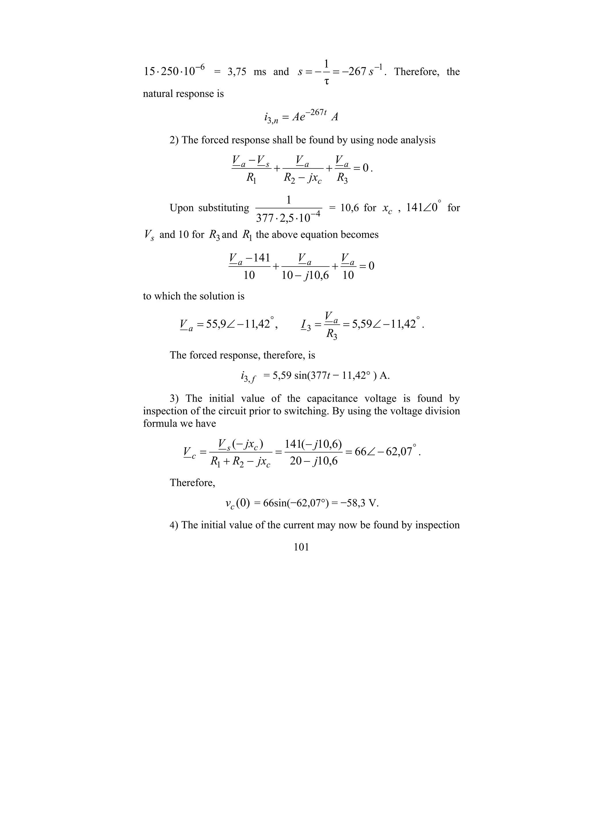
![103
found as a steady-state current in Fig. 2.17 after opening the switch
°
°
∠
=
−
∠
=
−
= 90
10
100
100
45
2
1000
j
jx
R
V
I
c
s
in which
Ω
=
⋅
=
= −
100
10
10
1
ω
1
5
3
C
xc
Thus,
f
i = 10 sin( 1000t + 90° ) A.
The initial value of the capacitance voltage (step 3) must be
evaluated in the circuit 2.17 prior to switching. By inspecting this
circuit, and noting that the resistance and the current source are short-
circuited, we may conclude that this voltage is equal to source voltage
)
0
(
)
0
( s
c v
v = .
By inspection of the circuit in Fig.2.17, we shall find the initial
value of current i (step4), which is equal to the current source flowing
in a negative direction, i.e., i(0) = − 4A. (Note that two voltage sources
are equal and opposed to each other.)
Finally the complete response (step 5) in accordance with
equation 2.17 will be:
A
e
t
e
i
i
i
t
i t
st
f
f 14
)
90
1000
sin(
10
)]
0
(
)
0
(
[
)
( 1000
−
°
−
+
=
−
+
= ,
where f
i (0) = 10sin90° = 10 A. Note that the period of the forced
current is
ms
π
2
s
10
π
2
1000
π
2 3
=
⋅
=
= −
T .
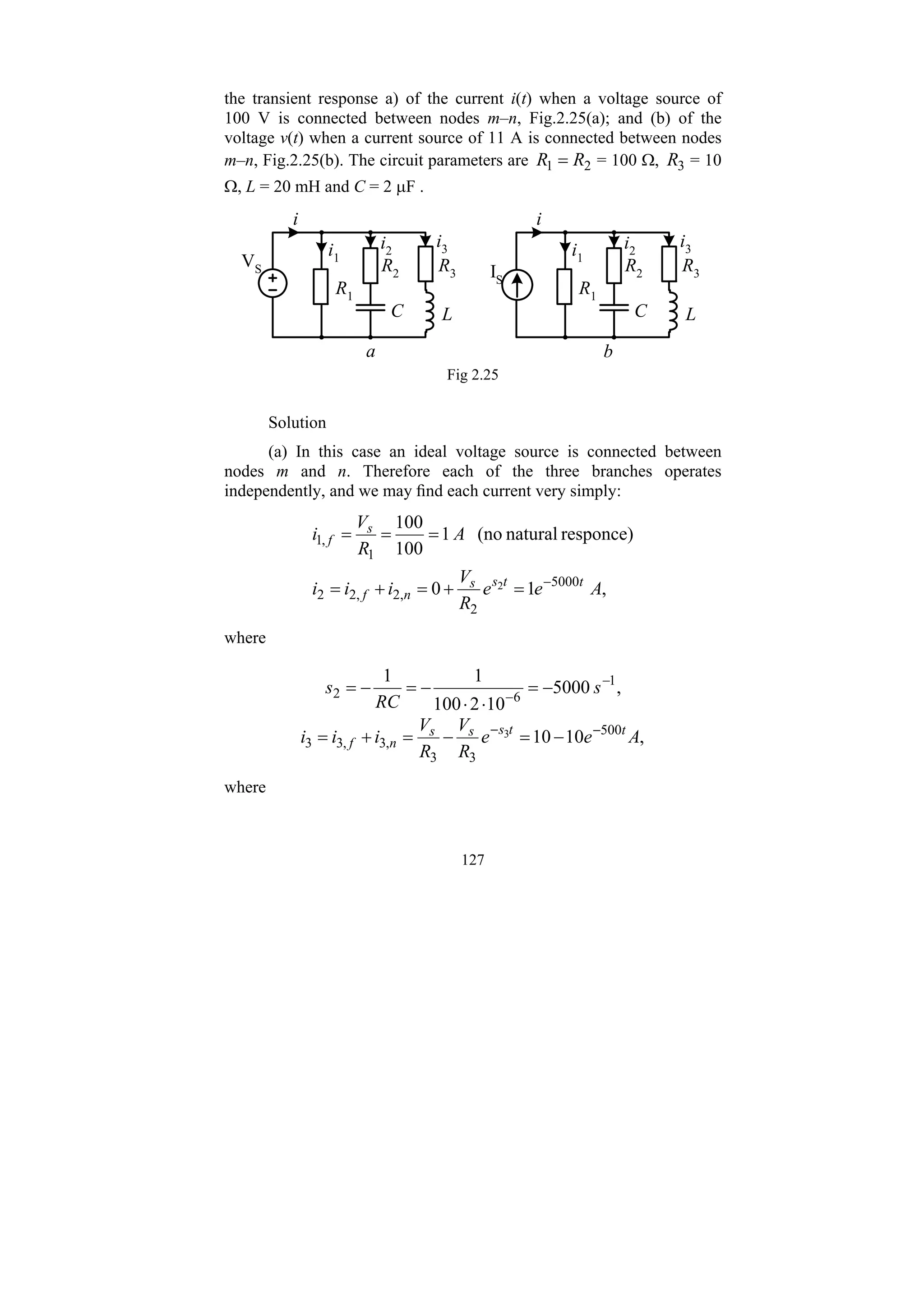
2.5. RLC CIRCUITS
This section is devoted to analyzing very important circuits
containing three basic circuit elements: R, L , and C. These circuits are](https://image.slidesharecdn.com/transientanalysisofelectricalpowercircuit-240923113814-129745da/75/Transient-Analysis-of-Electrical-Power-Circuit-pdf-103-2048.jpg)
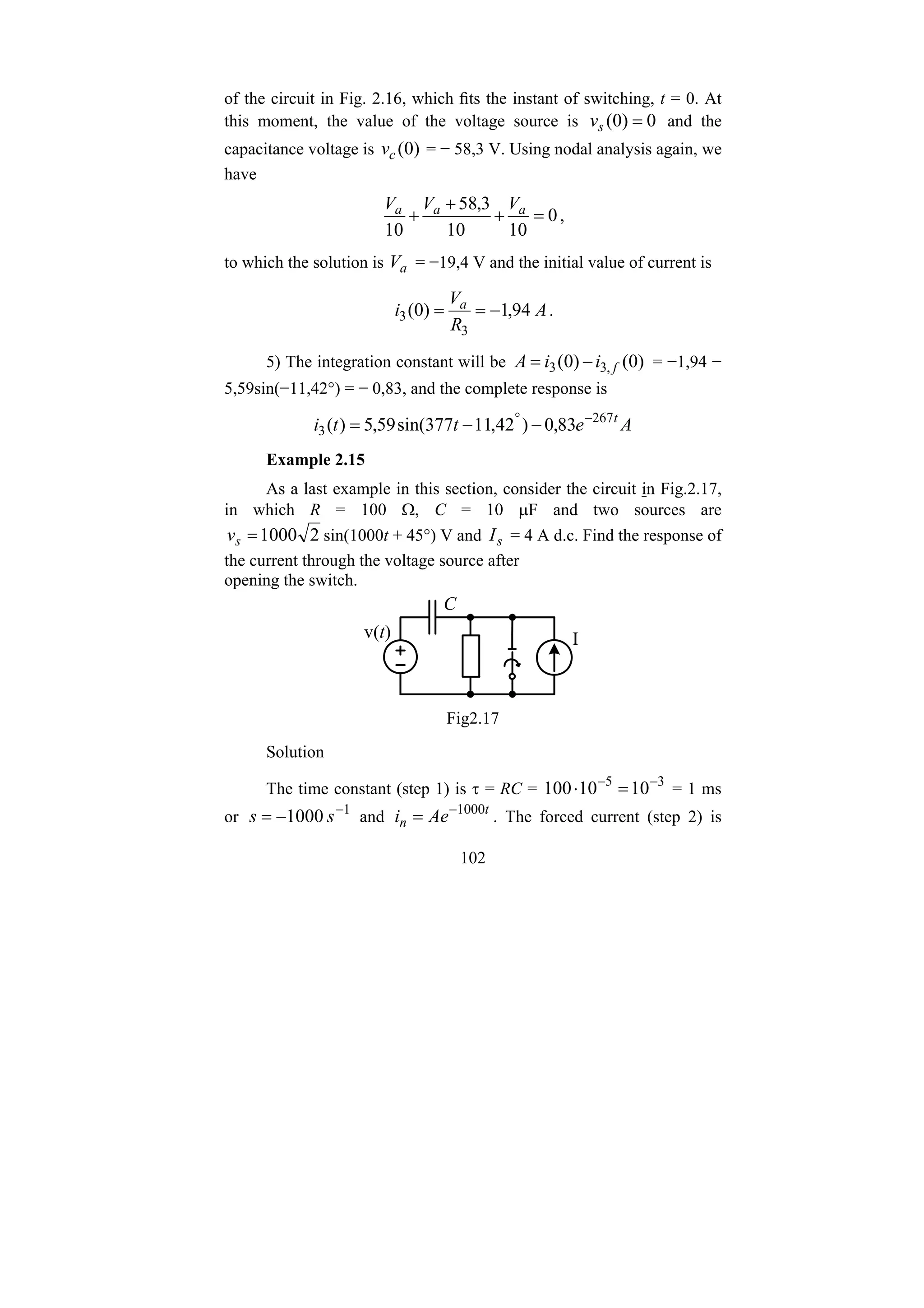
![105
characteristic equation. Let us determine the characteristic equation of
the circuit, shown in Fig. 2.18, depending on the kind of source: voltage
source or current source and on the place of its connection: (1) in series
with resistance 1
R , (2) in series with resistance 2
R , (3) between nodes
m–n.
R2
R3
L C
R1 R2
R3
L C
R1
a b
Fig.2.18
(1) Source connected in series with resistance 1
R
If a voltage source is connected in series with resistance 1
R , Fig.
2.18(a), we may use the input impedance method for determining the
characteristic equation. This impedance as seen from the source is
)
//(
1
)
( 3
2
1 sL
R
sC
R
R
s
Z +
⎟
⎠
⎞
⎜
⎝
⎛
+
+
= .
Performing the above operation and upon simplification and
equating Z(s) to zero we obtain
0
)
(
]
)
[(
)
(
3
1
3
1
3
2
2
1
2
2
1
=
+
+
+
+
+
+
+
+
R
R
s
L
C
R
R
R
R
R
R
LCs
R
R
(2.27)
and the roots of (2.27) are
LC
k
C
R
L
R
C
R
L
R
s
eq
eq 1
1
4
1
1
2
1
2
12
12
2
,
1 −
⎟
⎟
⎠
⎞
⎜
⎜
⎝
⎛
+
±
⎟
⎟
⎠
⎞
⎜
⎜
⎝
⎛
+
−
= .
where](https://image.slidesharecdn.com/transientanalysisofelectricalpowercircuit-240923113814-129745da/75/Transient-Analysis-of-Electrical-Power-Circuit-pdf-105-2048.jpg)
![107
0
1
1
1
1
3
2
1
=
+
+
+
+
=
sL
R
sC
R
R
Yin .
Performing the above operations and upon simplification, we
obtain
0
)
(
]
)
[(
)
(
3
1
3
1
3
2
2
1
2
2
1
=
+
+
+
+
+
+
+
+
R
R
s
L
C
R
R
R
R
R
R
LCs
R
R
(2.29)
Note that this equation (2.29) is the same as (2.27), which can be
explained by the fact that connecting the sources in these two cases does
not influence the configuration of the circuit : the voltage source in (1)
keeps the branch short-circuited and the current source in (3) keeps the
entire circuit open-circuited. In all the other cases the sources change the
circuit configuration.
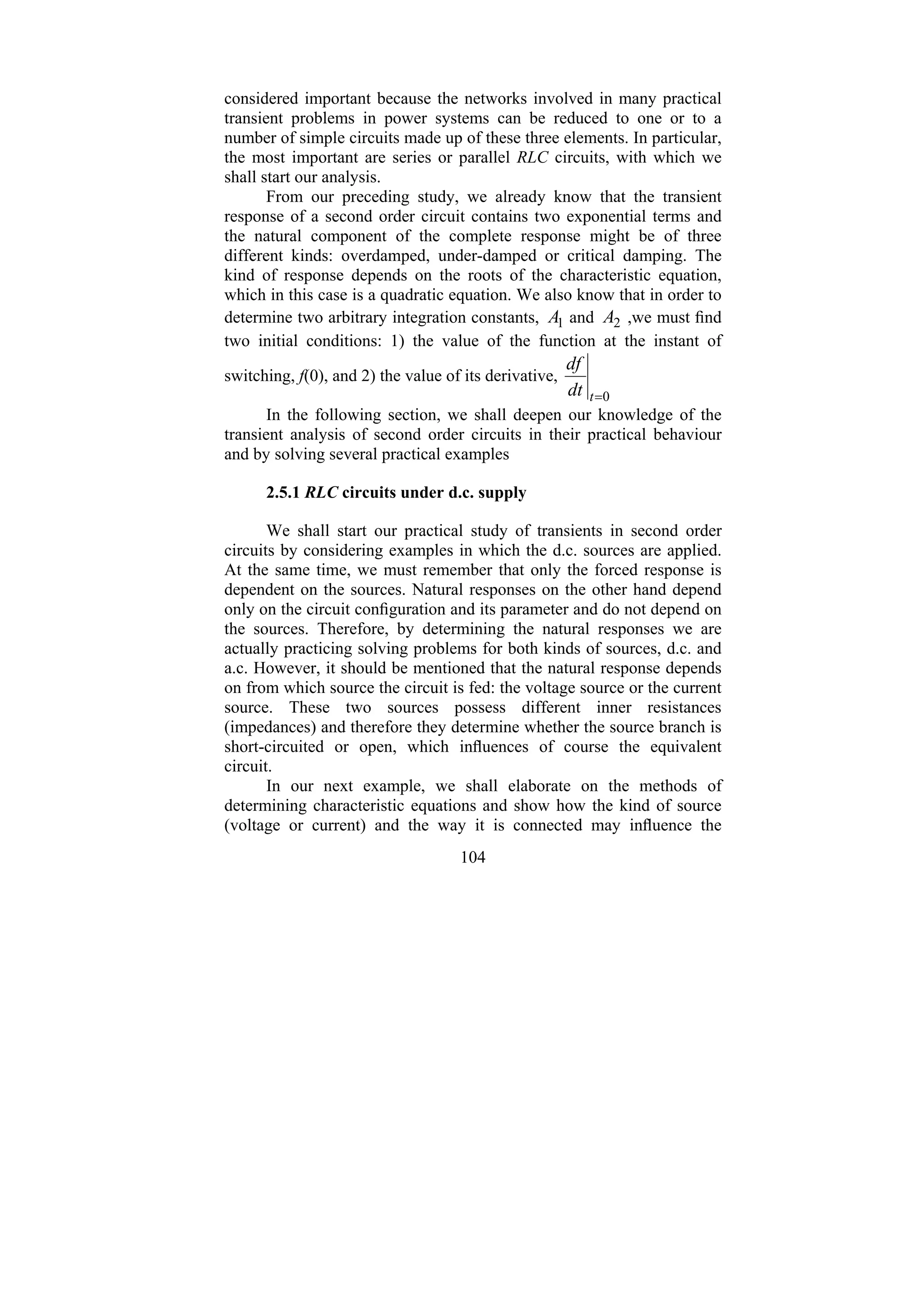
In the following analysis we shall discuss three different kinds of
responses: overdamped, underdamped, and critical damping, which may
occur in RLC circuits. Let us start with a free source simple RLC circuit.
(a) Series connected RLC circuits
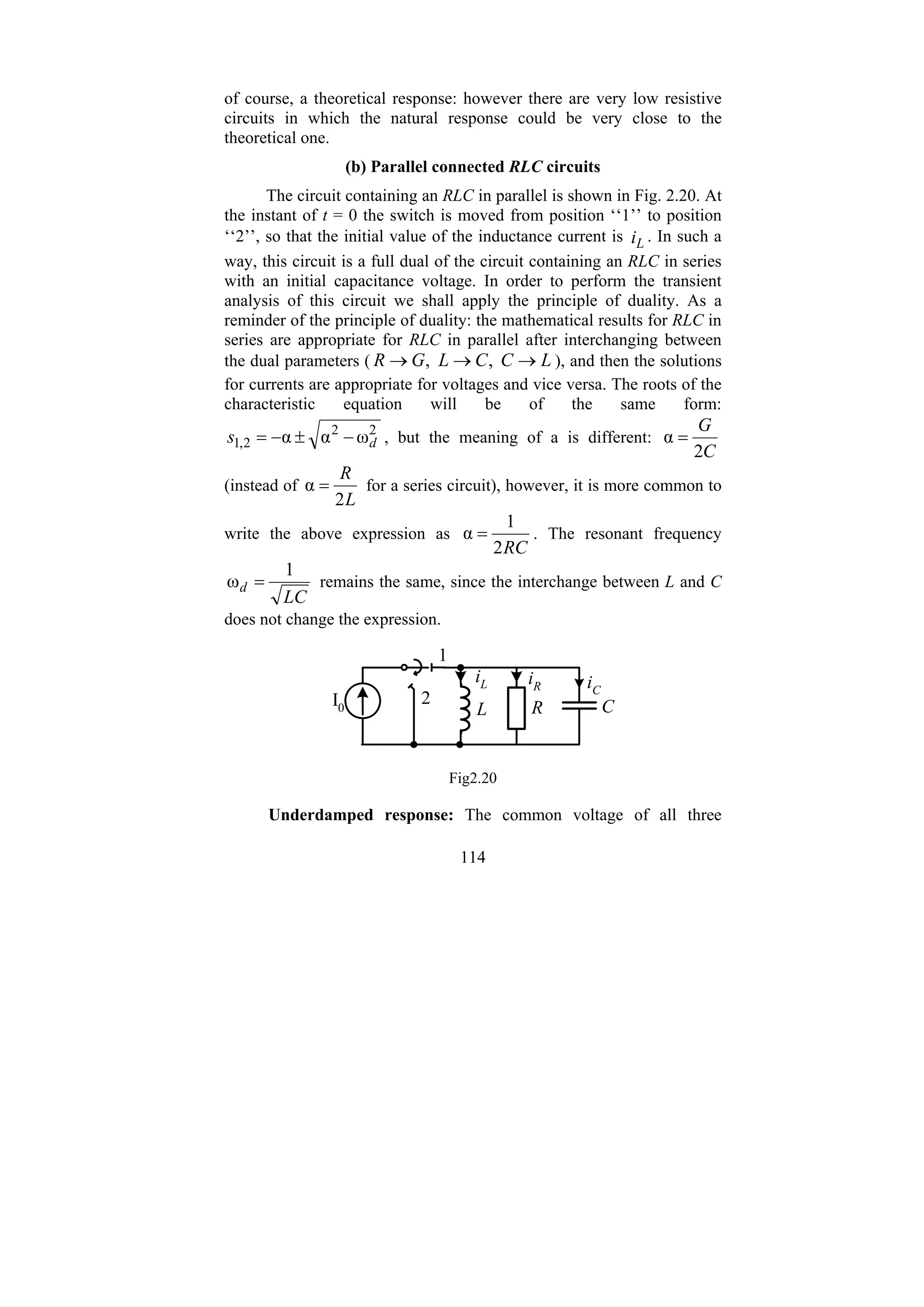
Consider the circuit shown in Fig. 2.19. At the instant t = 0 the
switch is moved from position ‘‘1’’ to ‘‘2’’, so that the capacitor, which
is precharged to the initial voltage 0
V , discharges through the resistance
and inductance. Let us find the transient responses of )
(t
vc , i(t) and
)
(t
vL .
R L
C
iC
V0
1 2
i
Fig.2.19
The characteristic equation is](https://image.slidesharecdn.com/transientanalysisofelectricalpowercircuit-240923113814-129745da/75/Transient-Analysis-of-Electrical-Power-Circuit-pdf-107-2048.jpg)
![118
which differs from equation 2.35 by the additional term due to the
initial value of the current 0
L
I . The current response will now be
( ) ( ),
)
(
)
( 2
1
2
1
2
1
1
2
0
1
2
0 t
s
t
s
L
t
s
t
s
c
n e
s
e
s
s
s
I
e
e
s
s
L
V
t
i −
−
+
−
−
= (2.53)
and the inductance voltage
( ) ( ),
)
( 2
1
2
1 2
2
2
1
1
2
0
2
1
1
2
0
,
t
s
t
s
L
t
s
t
s
c
n
L e
s
e
s
s
s
LI
e
s
e
s
s
s
V
t
v −
−
+
−
−
= (2.54)
The above equations 2.52–2.54 can also be written in terms of
hyperbolical functions. Such expressions are used for transient analysis
in some professional books. We shall first write roots 1
s and 2
s in a
slightly different form
2
2
2
,
1 ω
α
γ
γ
α d
s −
=
±
−
= (2.55a)
then
LC
s
s
s
s d
1
ω
γ
α
γ,
2 2
2
2
2
1
1
2 =
=
−
=
−
=
− ,
and
( ) ]
γ
sinh
γ
[cosh
α
γ
γ
α
γ
α
2
,
1
t
t
e
e
e
e
e
e
e t
t
t
t
t
t
t
s
±
=
+
=
= −
−
−
±
−
(2.55b)
With the substitution of equation 2.55(a) for 2
,
1
s and taking into
account the above relationships, after a simple mathematical
rearrangement, one can readily obtain
t
L
c
n
c e
t
C
I
t
t
V
t
v α
0
0
, γ
sinh
γ
γ
sinh
γ
α
γ
cosh
)
( −
⎥
⎦
⎤
⎢
⎣
⎡
+
⎟
⎟
⎠
⎞
⎜
⎜
⎝
⎛
+
= , (2.56)
and
t
L
c
n e
t
t
I
t
L
V
t
i α
0
0
γ
sinh
γ
α
γ
cosh
γ
sinh
γ
)
( −
⎥
⎦
⎤
⎢
⎣
⎡
⎟
⎟
⎠
⎞
⎜
⎜
⎝
⎛
−
+
−
= (2.57)](https://image.slidesharecdn.com/transientanalysisofelectricalpowercircuit-240923113814-129745da/75/Transient-Analysis-of-Electrical-Power-Circuit-pdf-118-2048.jpg)

![135
where
.
50
2
,
21
3
,
13
ω
1
5
,
51
2
,
48
7
,
37
30
ω
2
1
2
1
2
1
1
°
°
−
∠
=
+
+
=
−
=
=
∠
=
+
=
+
=
Z
Z
Z
Z
R
Z
j
C
j
Z
j
L
j
R
Z
in
Therefore,
.
)
50
377
sin(
2
2
,
47 A
t
if
°
+
=
The independent initial conditions are c
v (0) = 0, L
i (0) = 25,7
sin 43,3° = 17,6 A, since prior to switching:
.
3
,
43
40
7
,
37
tan
φ
7
,
25
7
,
37
40
2
1000
)
(
1
2
2
2
2
1
,
°
−
=
=
=
+
=
+
+
=
L
s
m
L
x
R
R
V
I
The next step is to determine the initial values of i(0) and
0
=
t
dt
di
.Since the input voltage at t = 0 is zero and the capacitance
voltage is zero, we have i(0) = [v(0) − c
v (0)]/R = 0. The initial value of
the current derivative is found with Kirchhoff ’s voltage law applied to
the outer loop
,
0
=
+
+
− c
s v
Ri
v ,
and, after differentiation, we have
.
62100
10
)]
88
(
533
[
10
1
1 3
0
0
0
=
−
−
=
⎟
⎟
⎠
⎞
⎜
⎜
⎝
⎛
−
=
=
=
= t
c
t
s
t dt
dv
dt
dv
R
dt
di
Here
3
0
10
533
ψ
cos
377
2
1000 ⋅
=
⋅
=
=
v
t
s
dt
dv
and](https://image.slidesharecdn.com/transientanalysisofelectricalpowercircuit-240923113814-129745da/75/Transient-Analysis-of-Electrical-Power-Circuit-pdf-135-2048.jpg)
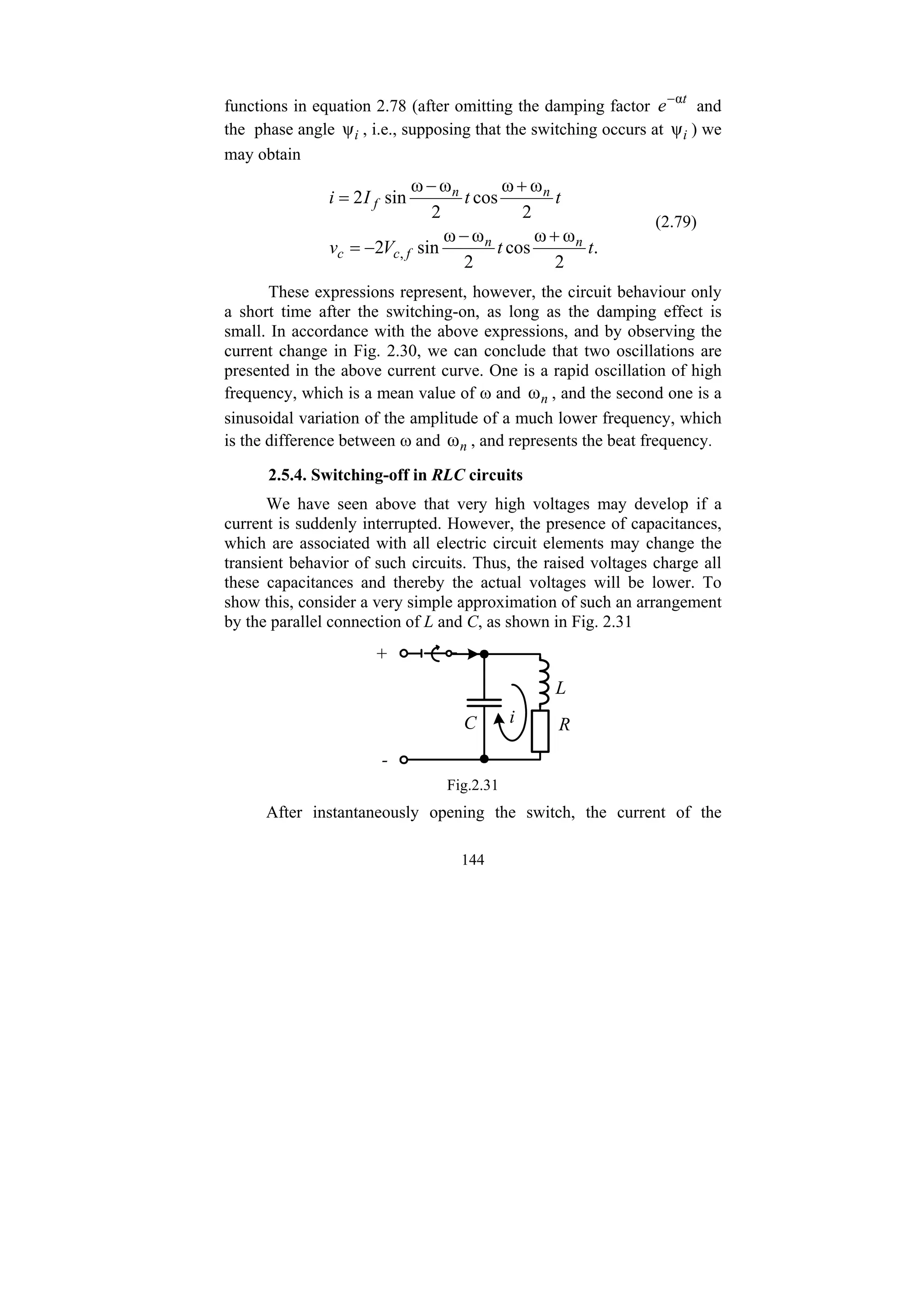
![138
R L
C
i
VS
LC
R <<
Fig.2.28
The natural response of the capacitance voltage will then be
β)],
ω
cos(
ω
β)
ω
sin(
α
[
)
ω
α
(
1
2
2
α
, +
−
+
−
+
=
=
−
∫ t
t
C
e
I
dt
i
C
v n
n
n
n
t
n
n
n
c
upon simplification, combining the sine and cosine terms to a common
sine term with the phase angle δ)
90
( +
°
,
δ),
90
(
β
ω
sin[
α
,
, +
−
+
= °
−
t
e
V
v n
t
n
c
n
c (2.61)
where
C
L
I
V n
n
c +
, , (2.62a)
n
ω
α
tan
δ 1
−
= , (2.62b)
and
.
1
ω
ω
α 2
2
2
LC
d
n +
=
+ (2.63)
The natural response of the inductive voltage may be found
simply by differentiation:
β)],
ω
cos(
ω
β)
ω
sin(
α
[
α
,
, +
+
+
−
=
= −
t
t
e
LI
dt
di
L
v n
n
n
t
n
n
L
n
L
or after simplification, as was previously done, we obtain](https://image.slidesharecdn.com/transientanalysisofelectricalpowercircuit-240923113814-129745da/75/Transient-Analysis-of-Electrical-Power-Circuit-pdf-138-2048.jpg)
![139
δ)].
90
(
β
ω
sin[
α
, +
+
+
= °
−
t
e
C
L
I
v n
t
n
n
L (2.64)
It is worthwhile to note here that by observing equation 2.61 and
equation 2.64 we realize that n
c
v , is lagging slightly more and n
L
v , is
leading slightly more than 90° with respect to the current. This is in
contrast to the steady-state operation of the RLC circuit, in which the
inductive and capacitive voltages are displaced by exactly ± 90° with
respect to the current. The difference, which is expressed by the angle δ
,is due to the exponential damping. This angle is analytically given by
equation 2.62b and indicates the deviation of the displacement angle
between the current and the inductive/capacitance voltage from 90°.
Since the resistance of the resonant circuits is relatively small, we may
approximate
C
L
R
LC
L
R
LC
n
2
δ
1
2
1
ω
2
≅
≅
⎟
⎠
⎞
⎜
⎝
⎛
−
= . (2.65)
For most of the parts of the power system networks resistance R
is much smaller than the natural impedance
C
L so that the angle d is
usually small and can be neglected.
By switching the RLC circuit, Fig. 2.28, to the voltage source
)
ψ
ω
sin( v
m
s t
V
v +
= (2.66)
the steady-state current will be
)
ψ
ω
sin( i
f
f t
I
i +
= (2.67)
the amplitude of which is
2
2
ω
1
ω ⎟
⎠
⎞
⎜
⎝
⎛
−
+
=
C
L
R
V
I m
f , (2.68)](https://image.slidesharecdn.com/transientanalysisofelectricalpowercircuit-240923113814-129745da/75/Transient-Analysis-of-Electrical-Power-Circuit-pdf-139-2048.jpg)
![143
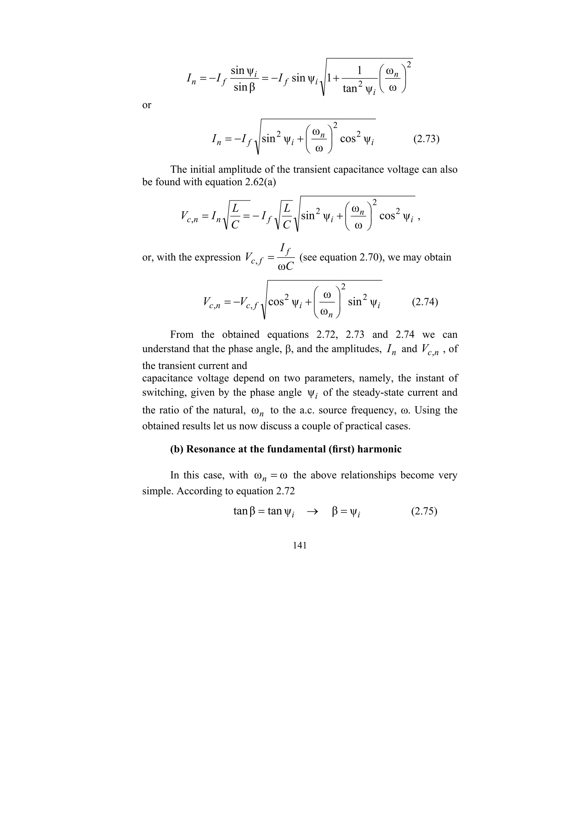
(c) Frequency deviation in resonant circuits
In this case, equations 2.75 and 2.76 can still be considered as
approximately true. However since the natural and the system
frequencies are only approximately (and not exactly) equal, we can no
longer combine the natural and steady-state harmonic functions and the
complete response will be of the form
[ ]
[ ].
)
90
ψ
ω
sin(
)
90
ψ
ω
sin(
)
ψ
ω
sin(
)
ψ
ω
sin(
α
,
α
°
−
°
−
−
+
−
−
+
=
+
−
+
=
i
n
t
i
f
c
c
i
n
t
i
f
t
e
t
V
v
t
e
t
I
i
(2.78)
Since the natural current / capacitance voltage now has a slightly
different frequency from the steady-state current / capacitance voltage,
they will be displaced in time soon after the switching instant.
Therefore, they will no longer subtract as in equation 2.77, but will
gradually shift into such a position that they will either add to each other
or subtract, as shown in Fig.2.30.
i
0 t
Fig.2.30
As can be seen with increasing time the addition and subtraction
of the two components occur periodically, so that beats of the total
current / voltage appear. These beats then diminish gradually and are
decayed after the period of the 3–5 time constant. It should also be noted
that, as seen in Fig. 2.30, the current/capacitance voltage soon after
switching rises up to nearly twice its large final value; so that in this
case switching the circuit to an a.c. supply will be more dangerous than
in the case of resonance proper. By combining the trigonometric](https://image.slidesharecdn.com/transientanalysisofelectricalpowercircuit-240923113814-129745da/75/Transient-Analysis-of-Electrical-Power-Circuit-pdf-143-2048.jpg)


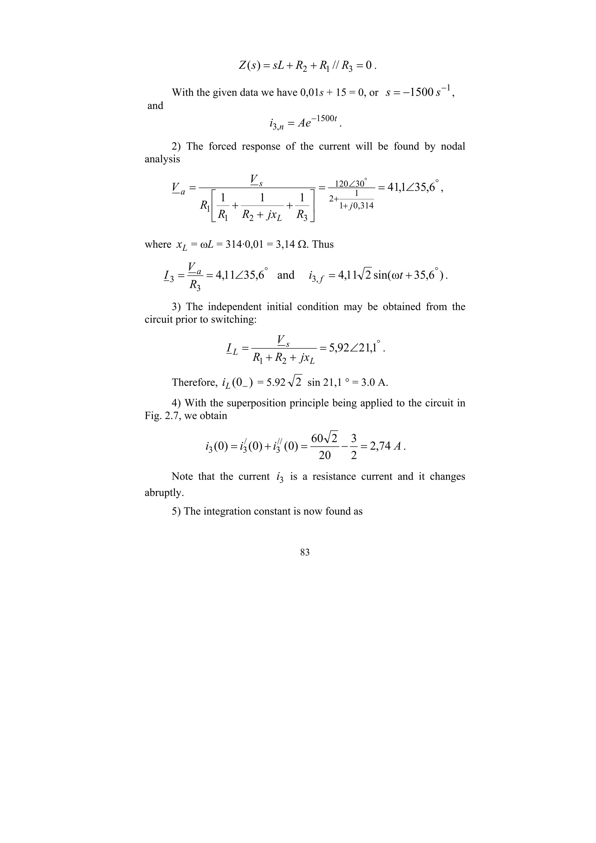
![[Juan Martinez] Transient Analysis of Power Systems.pdf](https://cdn.slidesharecdn.com/ss_thumbnails/juanmartineztransientanalysisofpowersystems-220712220132-46430ea1-thumbnail.jpg?width=640&height=640&fit=bounds)