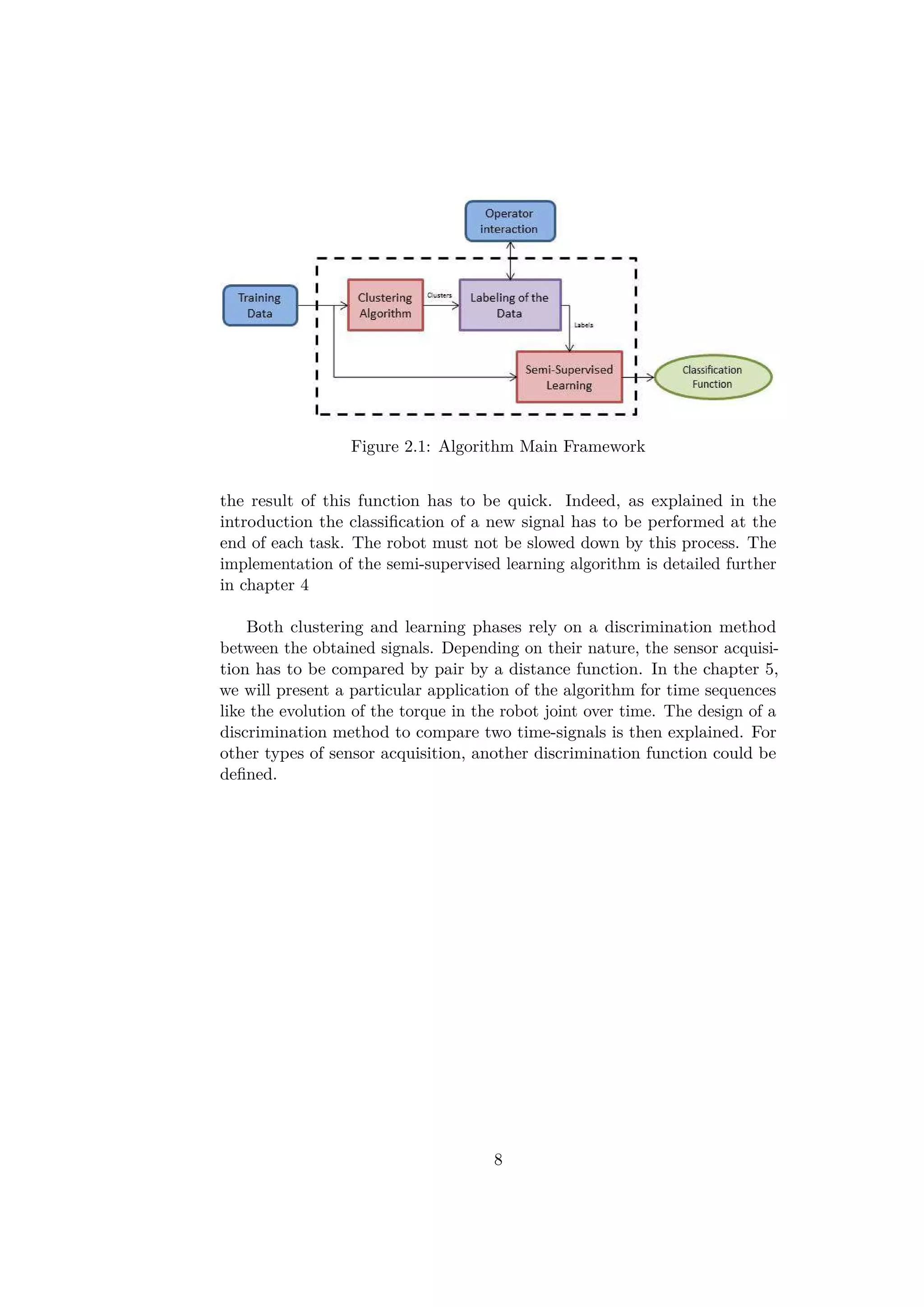
This document is a master's thesis submitted by Jérémy Pouech at KTH Royal Institute of Technology in Stockholm, Sweden in 2015. The thesis proposes an algorithm to make failure detection and classification for industrial robots more generic and semi-automatic. The algorithm uses machine learning to analyze sensory data recorded during robot operations and learn to differentiate between success and failure scenarios. It clusters the training data using OPTICS clustering and extracts labels to learn a classification function to detect failures in new data. The goal is to allow operators without programming skills to teach failure detection to robots. The thesis applies this framework to detect failures in an assembly task performed by an ABB YuMi robot.


![Chapter 1
Introduction
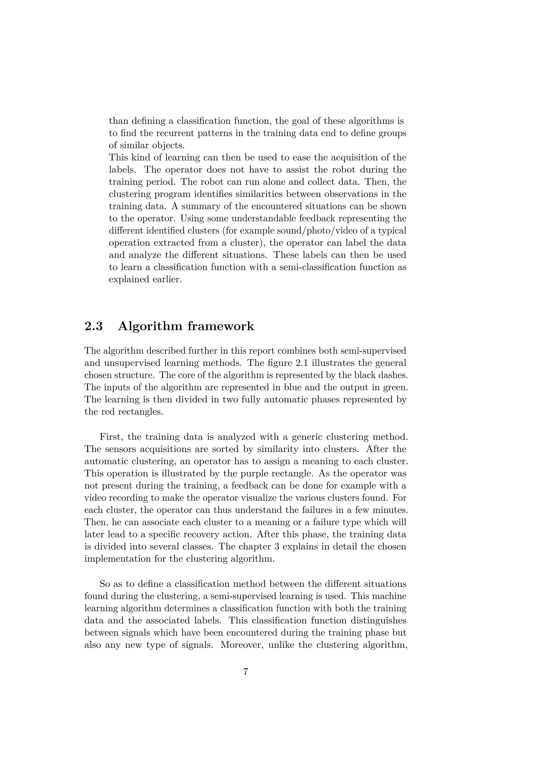
The master’s thesis presented in this paper deals with issues encountered in
industrial robotics. In this introduction, a first part concerns the general
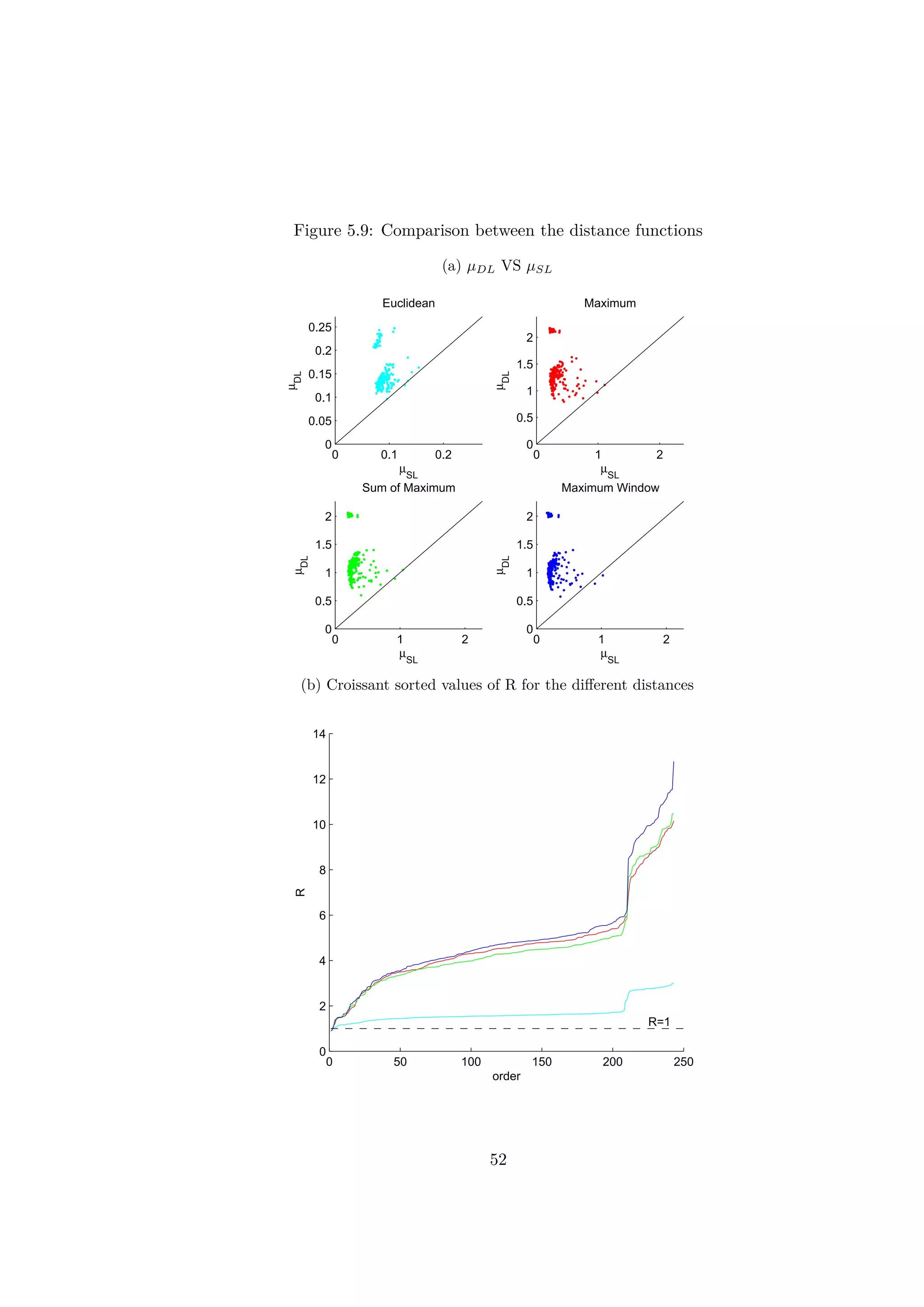
background about assembly line robots in the industry. Then some prob-
lematics linked to the installation and the programming of such robots are
explained. Finally some goals are introduced so as to understand the current
industrial interests in that field.
1.1 Background
Since their creation in the early 19th century, the assembly lines aim to
increase the productivity in factories. To be as efficient as possible, the
activity is divided in small and repetitive tasks performed by low-qualified
workers. This way of organizing a factory has been proved to be effective and
has allowed the beginning of massive productions lines. However, the gain of
productivity came at the cost of bad working conditions. A job in a factory
is limited to repetitive tasks that are often boring, tiring and stressful for a
human. The job in factories has become degrading and unpleasant.
Nowadays, the newly-built factories tend to equip their assembly lines
with machines and robotized agents. The robots are designed so as to help
the workers in the most repetitive and tiresome actions. The future place of
robots in assembly lines can be seen as a powerful tool for workers ([1, 2, 8]).
Unlike the commonplace image of robots which can entirely substitute a
human, the idea is to create intelligent agents able to co-operate hand in
hand with human colleagues. Then, workers would become robot coaches.
They would be able to teach operations without special education. The
conditions of work in factories as well as the efficiency of the lines would be
raised by this robotic revolution.
However, those objectives raise numerous technical problems. Currently,
1](https://image.slidesharecdn.com/ff3a18c7-0e8d-4852-b4ba-9bdc3c906b26-151031192058-lva1-app6892/75/Thesis_Report-10-2048.jpg)
![it is difficult to communicate with an industrial robot. Most of them can
only understand lines of codes written by programmers. Their integration
in assembly line remains technical, takes a long time and is reserved for
experts. The written program is often definitive and cannot be changed by
an untrained laborer working next to it.
This thesis is part of a research work which aims to improve the usability
of industrial robots by humans. The current researches have made attempts
to automate the programmers’ work and to create simple interfaces for
the future robot coaches. To ensure that every worker without special
programming skills manages to teach a robot, the interfaces have to be
simple and intuitive. Some recent works have shown it is possible to teach a
robot by holding its arms and moving them as a puppet. The movements
of the robotic arm are recorded and then are repeated in a loop in order
to perform the taught operation ([2]). This robot teaching is an efficient
method to automate one of the first parts of the work done by a robot
programmer. Following this same idea, this report presents an efficient
algorithm which makes an operator able, without writing any line of code,
to modify the behavior of the robot in order to increase the robustness in
the robot operations.
1.2 The search for robustness
A large part of the robot programmers’ job is to make the machine ro-
bust during its operations. The assembly task given to the robot has to
be successful most of the time since the robot has to be as productive as
possible. However, after the programming of a standard behavior, the robot
is rarely fully successful in all the operations. Due to some irregularities of
the pieces to assemble (different stiffness, previous malformation, etc.) or
sensor measurement errors, the robot will have to deal with failures in the
assembly. Those failures have to be detected and taken into account in the
robot program. A flawed piece which continues its path in the assembly
process can lead later to some bigger failures in the entire process, causing a
significant efficiency loss in the assembly line afterwards.
To create a robust failure detection, the programmer has to study the
robot operation and analyze the nature and the cause of the failures. Most
of the time, he has to look deep down into the signals from the sensors
integrated in the robot to find a way to produce a feedback for each assembly
problem. Then, for each problem detected, the programmer can implement
a recovery action. A recovery action can be either a new movement to fix
a problem in the assembly or simply a rejection operation to eliminate the
flawed object and give it to a more experienced human. As the tasks are most
2](https://image.slidesharecdn.com/ff3a18c7-0e8d-4852-b4ba-9bdc3c906b26-151031192058-lva1-app6892/75/Thesis_Report-11-2048.jpg)

![Chapter 3
The clustering of the training
data
In order to ease the acquisition of training data labels by the operator, the
research for similarities between sensor acquisitions can be automated. This
operation is performed by a clustering algorithm which is presented in this
chapter. In a first part, the literature on the subject is presented. Then the
principle of the chosen algorithm is detailed. Finally we will explain how the
hierarchical clustering can help an operator to label quickly the training data.
3.1 Related work on clustering
One of the most well-known clustering algorithms is called the k-mean ([17]).
Its principle involves calculating k average signals which are the most repre-
sentative of the data set. This calculation is done by an iterative method.
Some variations of this algorithm exist such as the k-medoid [14] or the c
fuzzy mean [6]. Another algorithm named CURE [12] aims to find a hier-
archical structure in the data. These algorithms can hardly be used in the
presented application because one of their inputs is the number of desired
clusters. In our case, the data is entirely unknown and the number of types
of failure is difficult to predict.
Another approach to clustering is to look at the density of objects in a
neighborhood of the k closest signals. Those methods similar to the KNN
classification methods are explored in the literature as well. The principle
is to create a cluster when the density of objects is high. For example, in
a set of points in a 2d-space, a cluster would be created where the points
are numerous in a delimited area. The most popular algorithm using this
method is DBSCAN [11]. This algorithm only needs two parameters to be
tuned: Minpts and . It processes object by object the number of neigh-
9](https://image.slidesharecdn.com/ff3a18c7-0e8d-4852-b4ba-9bdc3c906b26-151031192058-lva1-app6892/75/Thesis_Report-18-2048.jpg)
![boring objects separated by a distance lower than . If the neighborhood
contains at least Minpts objects, the objects are part of the same cluster.
The principle is simple however the algorithm is very sensitive to the choice
of and Minpts. Changing the parameters can lead to totally different
clusters. Then, they have to be determined very wisely depending on the
data set. As the training data in our application is relatively small, the
parameter for DBSCAN can hardly be tuned properly.
On the same idea of clustering by density, another method called OPTICS
is very similar to DBSCAN (see [5]). It involves processing an order for the
different objects in the training data so as to make a clustering operation
easier. The article about OPTICS then proposes a clustering algorithm
based on the preprocessed order. This last method has been chosen and
implemented for our algorithm.
3.2 Principle of OPTICS
As mentioned before, the chosen algorithm is OPTICS and is described in
the article [5]. The definition of clusters is similar to the one for DBSCAN
but the implementation to find them is different. The algorithm provides an
ordering of objects which allows a comprehensive representation of a complex
set of data in 1D. The ordering makes it possible to find a hierarchical
clustering, that is to say a complex structure containing several levels of
clusters. A cluster can contain smaller clusters in its inside. The structure
can be represented as a tree where each branch means a particular set of
common points between the signals. The lower are the branches in the tree,
the closer are the objects clustered.
3.2.1 Density-based clusters
The methods OPTICS and DBSCAN are two density-based clustering algo-
rithms. We present in this section necessary concepts to define mathemati-
cally a cluster with this clustering approach.
The general idea of this kind of clustering is to look at the distances
between the objects of the data set. It supposes then that a discrimination
method which gives a distance score between each pair of objects is available.
Depending on the objects nature, this distance can be processed by various
ways. If the object can be described with specific features, the distance
function can be for example the Euclidean distance between the points
representing the objects in the feature space. For other types of objects, it is
easier to define a distance directly with the digital values of the object. The
chapter 5.2 will give an example of research for an efficient distance function
between time signals using the taken values over time. In order to illustrate
10](https://image.slidesharecdn.com/ff3a18c7-0e8d-4852-b4ba-9bdc3c906b26-151031192058-lva1-app6892/75/Thesis_Report-19-2048.jpg)
![Figure 3.1: Density-reachability and connectivity
(Figure extracted from [5])
determine the neighborhood of an object is the Euclidean distance in the
2-d feature space.
3.2.2 Density-based Ordering
Definitions of notions
The algorithm DBSCAN consists in finding the clusters as defined previously
for the given parameters MinPts and . However, as mentioned before, the
algorithm is very sensitive to a change of parameters, in particular for the
parameter . This parameter can be seen as the maximum tolerated distance
between the objects in a cluster. A decrease of leads to smaller clusters in
which the objects are closer to another and so have more similarities. On
the contrary, if is increased then the clusters are wider and include further
objects. The idea of the algorithm OPTICS is to find a representation of the
objects so as to find all the levels of similarities corresponding to different
values of .
The sorting method OPTICS is based on two distances: the core-distance
and the reachability-distance which are defined as follows:
Core-distance
The core-distance is calculated for each object and represents how far
the neighboring objects are from this first object. Let ω be an object in
the database Ω. The core-distance CD(ω) is equal to the distance of the
Minptsth nearest neighbors called as well Minpts-distance(ω):
CD(ω) = Minpts-distance(ω) (3.4)
This core-distance corresponds to the minimum value of such that an object
can be considered as a core-object and thus generate a cluster.
Reachability-distance
The reachability-distance is an asymmetric distance between two objects.
Let d(ω, ν) the chosen distance to differentiate between ω and ν. The
12](https://image.slidesharecdn.com/ff3a18c7-0e8d-4852-b4ba-9bdc3c906b26-151031192058-lva1-app6892/75/Thesis_Report-21-2048.jpg)
![reachability-distance RD(ω) is defined as:
RD(ω, ν) = max(CD(ν), d(ω, ν)) (3.5)
This distance corresponds to the minimum value of for which ω is directly
density-reachable from ν. That is to say, if ≥ RD(ω, ν), ν is a core-object
and ω is in the -neighborhood of ν.
These definitions found in the article [5] can be restricted. The neigh-
borhood query in large databases can be restrained to a maximum distance.
This limitation is not very important in our use case because the data base
used is relatively small and the execution time is not very limiting. The
definition presented here is the extension of the definition in [5] when this
maximum distance tends to +∞.
The notion of core-distance and reachability-distance are illustrated in
the figure 3.2 for a few objects in a 2d-space. In this graph, MinPts is
equal to 3. The Core-distance of the point o is represented by the inner
circle whose radius is equal to the distance of the third neighbor of o. The
Reachability-distance of p1 from o is equal to the Core-distance of o since
p1 is in the neighborhood of o. p2 is not in the neighborhood of o, so the
Reachability-distance of p2 from o is equal to the distance between the two
points. The distance M on the figure is the maximum distance that a point
can have from o to be in the neighborhood of o. In the following, we will fix
this maximum value M to infinity.
The Ordering Algorithm
The goal of the sorting is to create an order of the objects which represents
their proximity and their capacity to create clusters according to the definition
given earlier. During the ordering, the algorithm treats the objects one by
one and places them in the ordered list by smallest reachability distance
from previously processed points. The algorithm follows the steps as below:
Initialization
First, a temporary list is created containing all the objects to order. This
list will be called seeds_list. Aside, a value is associated to every object.
This value will represent the minimum reachability distances RD∗ of the
point from all the points already placed in the sorted list. These values are
initialized to infinity and updated during the ordering with smaller values
encountered. Finally, an empty list ordered_list is created. This list will
contain the sorted objects.
13](https://image.slidesharecdn.com/ff3a18c7-0e8d-4852-b4ba-9bdc3c906b26-151031192058-lva1-app6892/75/Thesis_Report-22-2048.jpg)
![Figure 3.2: Core-distance and Reachability-distance
(Figure extracted from [5])
Iteration
The element corresponding to the smallest reachability distance RD∗ is
removed from the seeds_list and placed in ordered_list. Note that for the
first iteration, one element will be picked randomly.
The reachability distances of all the elements in the seeds_list from the
picked object are processed. The reachability-distance RD∗ of the objects
still in the seeds_list is updated if the processed value is smaller.
End of the process
The algorithm ends when all the elements in the seeds_list have been
processed.
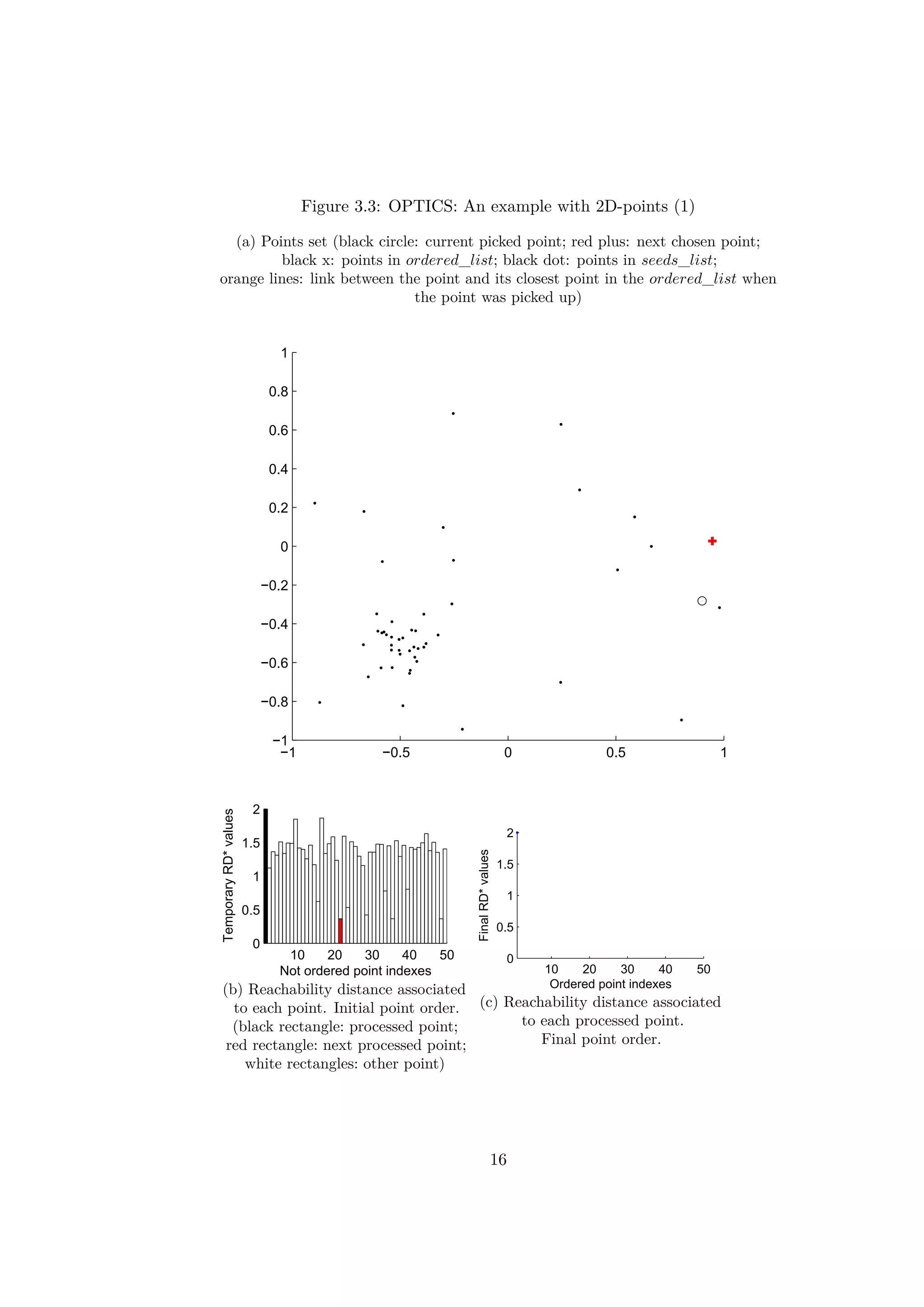
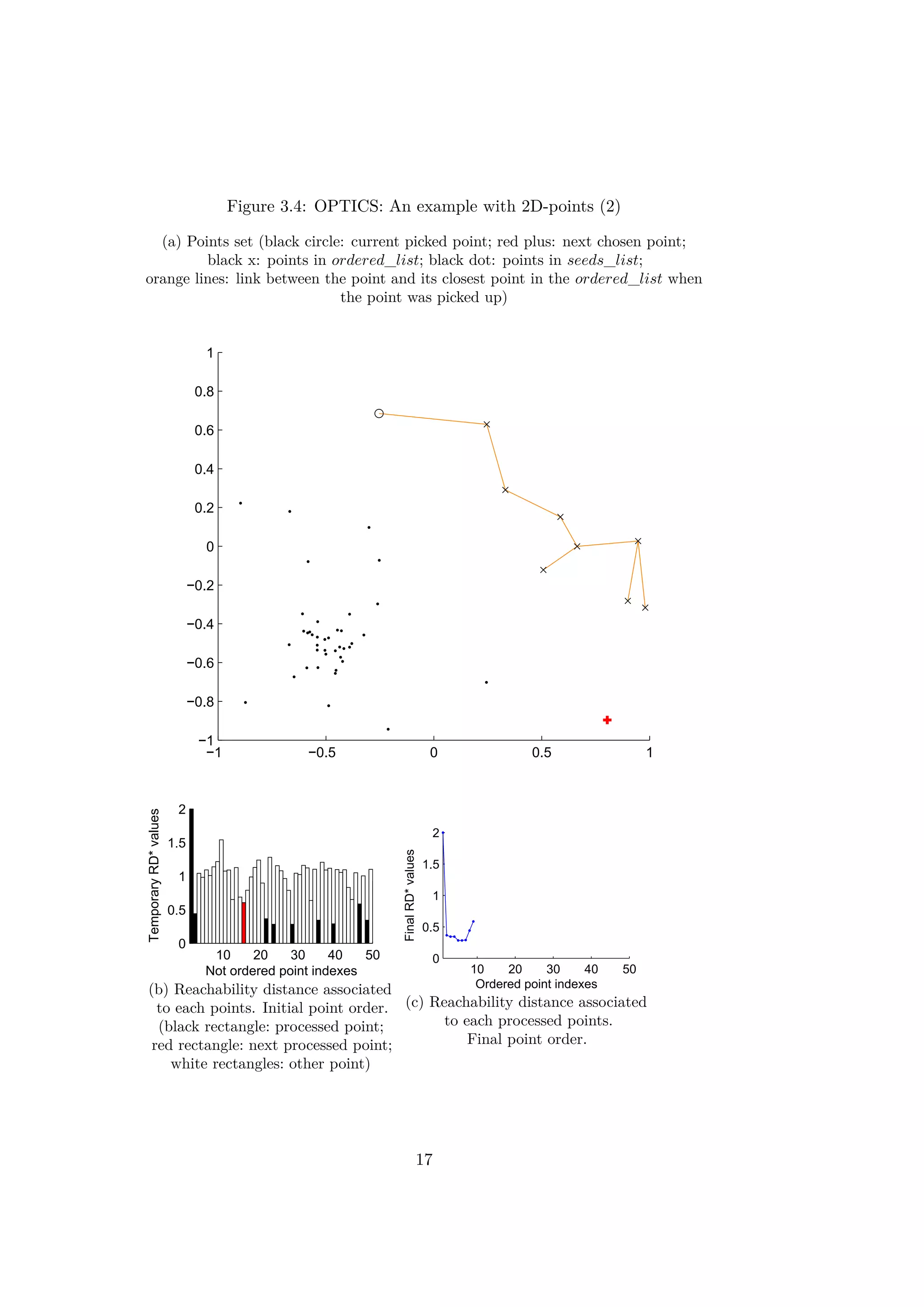
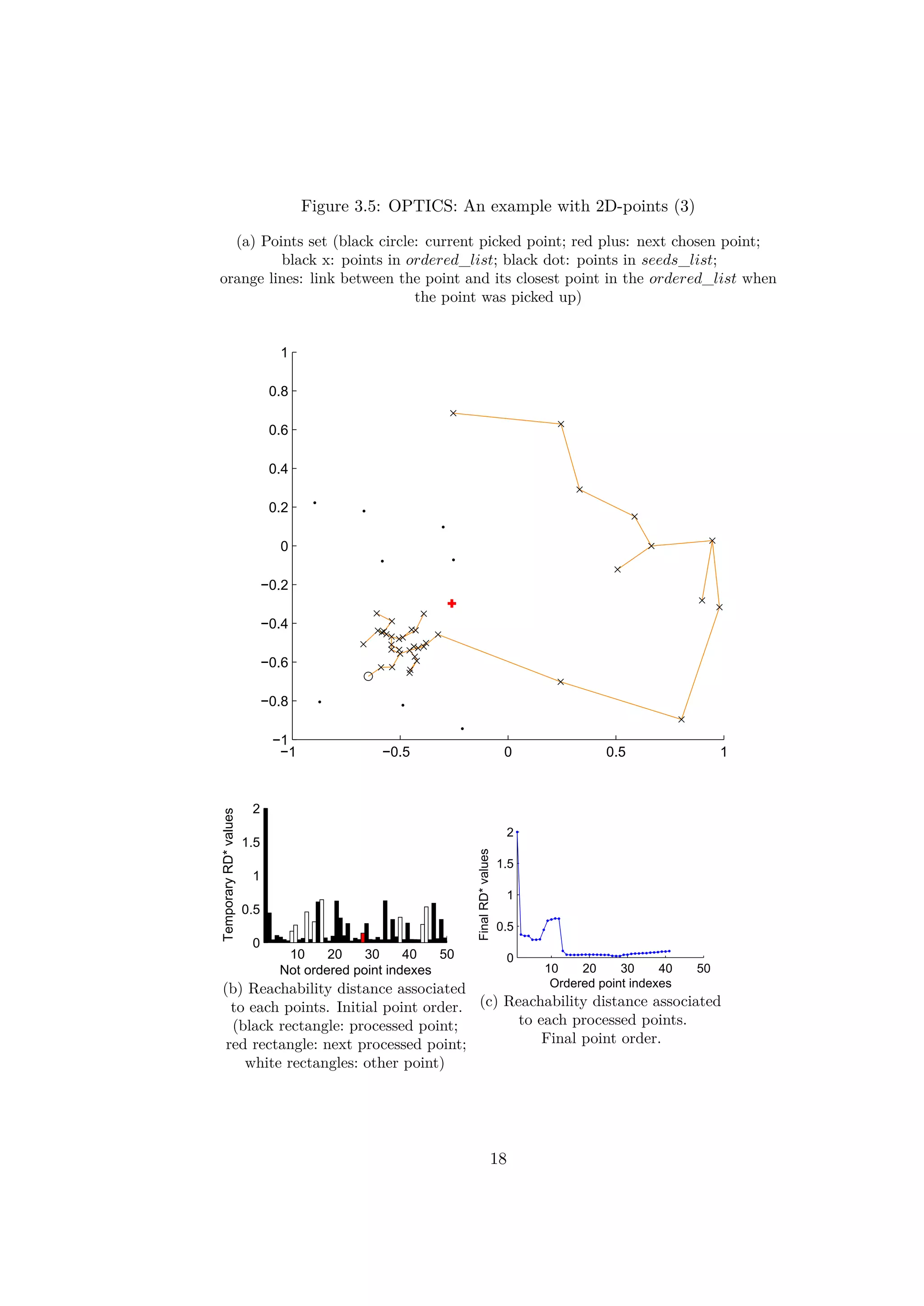
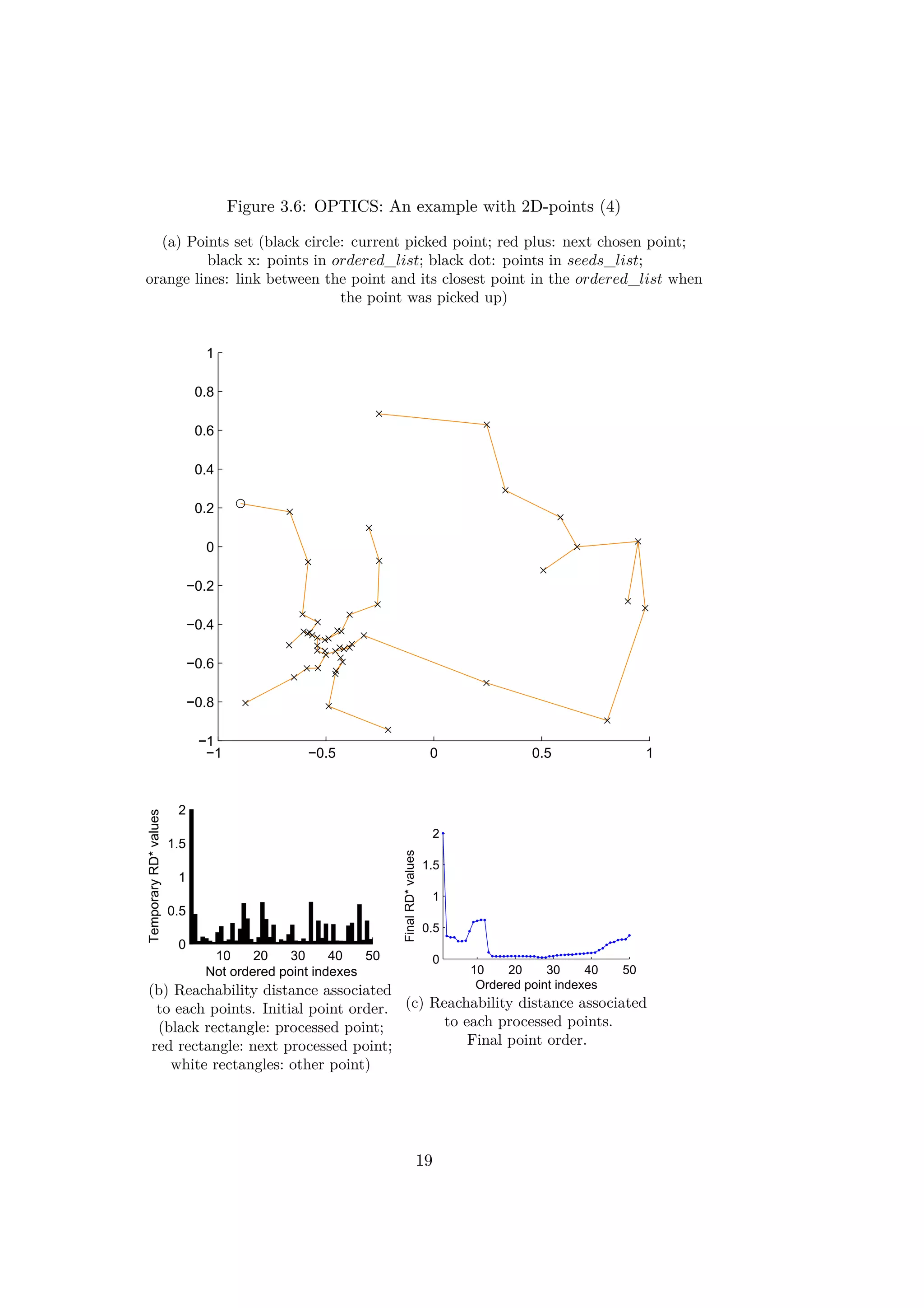
The figures 3.3, 3.4, 3.5 and 3.6 illustrate different iterations of the
algorithm for a simple example with 2d-points. At first the points are placed
in the seeds_list randomly. The rectangles in the figures 3.3b, 3.4b, 3.5b
and 3.6b represent the values of the reachability distances from previous
points. The order of the points is the initial random order.
The results of the first iteration are illustrated on the figure 3.3. One point
(represented by a circle) is picked in the seeds_list. Here, the first point has
been picked. All the reachability distances are updated on the figure 3.3b.
Previously infinity, the values are now finite except the first elements which
will never be updated. A first blue point has been placed in the graph on
the figure 3.3c.
After around ten iterations, the values of RD∗ decrease progressively as
14](https://image.slidesharecdn.com/ff3a18c7-0e8d-4852-b4ba-9bdc3c906b26-151031192058-lva1-app6892/75/Thesis_Report-23-2048.jpg)
![0 10 20 30 40 50
0
0.1
0.2
0.3
0.4
0.5
0.6
0.7
order
RD*
Figure 3.7: Reachability-Distances and Core-Distances of the 2D-points
ordered by OPTICS
(Blue for RD∗, red for CD)
3.2.3 A clustering method with OPTICS
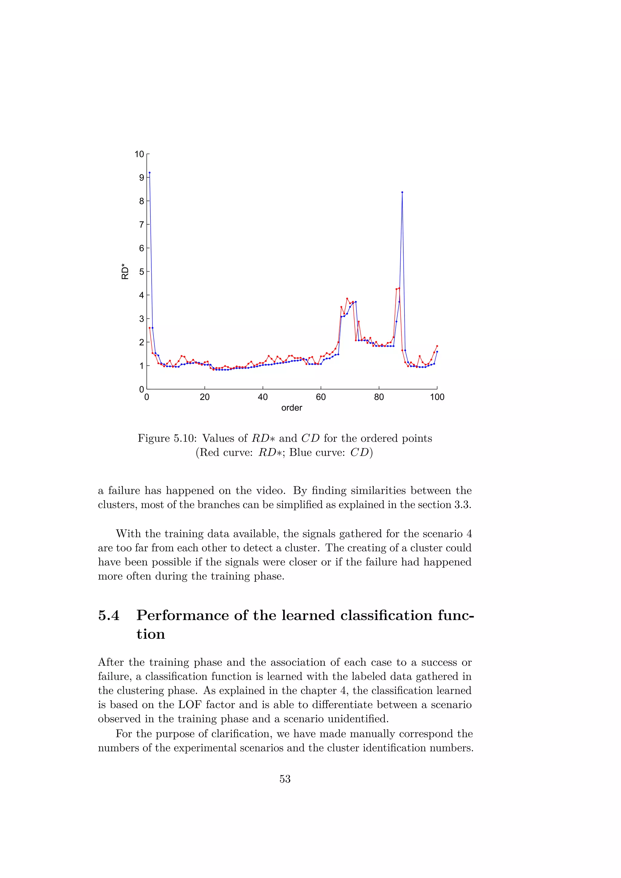
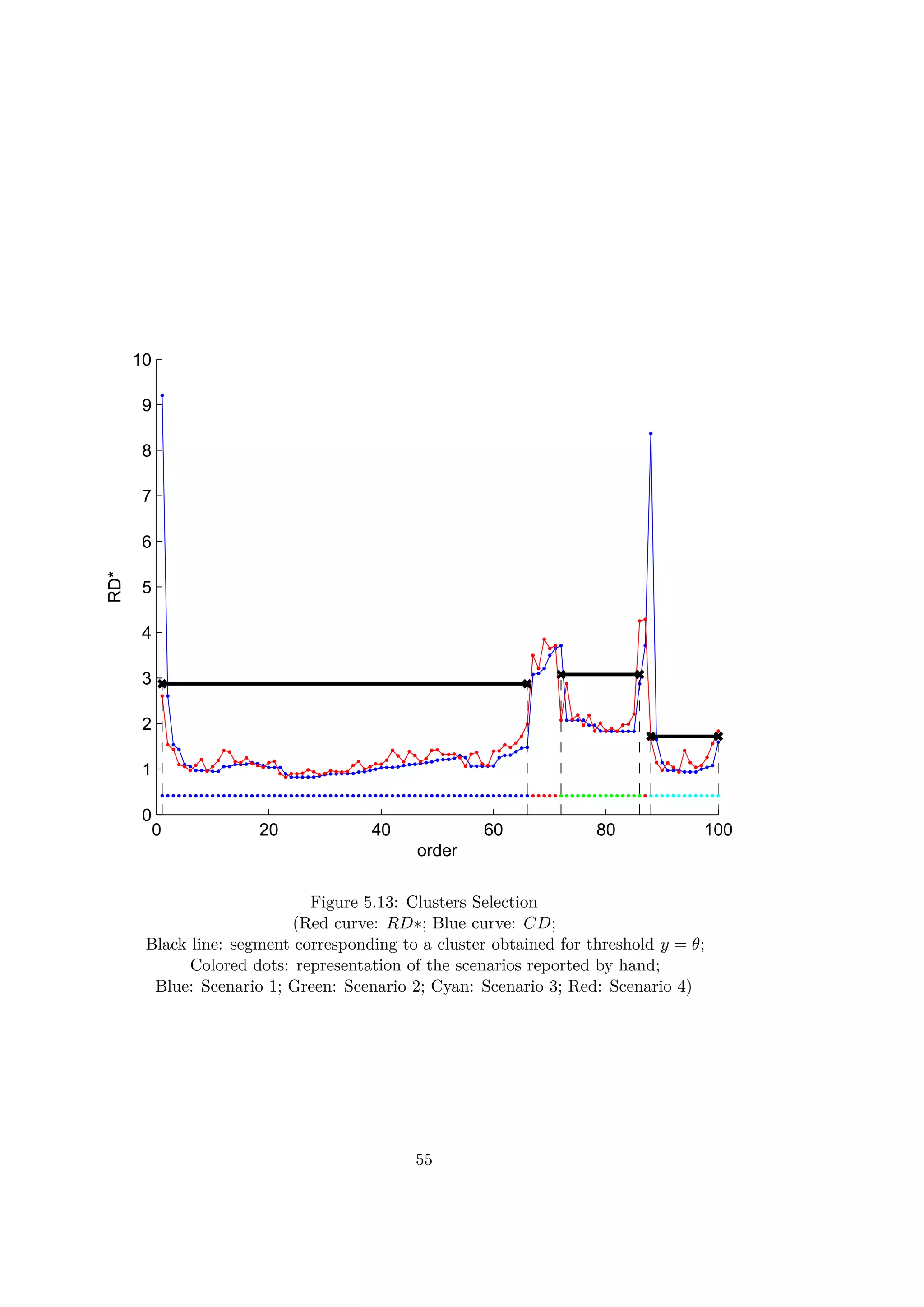
Intuitively, when a sequence of RD∗ values are locally small, the correspond-
ing objects are close to each other and can be part of the same cluster. A
rising slope means a higher distance between all the previous points and the
next ones and so the end of a cluster. A decreasing slope shows the beginning
of a new cluster. In the article [5], a method based on the values of RD∗
and CD is presented in order to find a DBSCAN equivalent clustering. The
parameter in DBSCAN can be seen as a threshold for the RD∗ curves. A
segment of consecutive indexes which have RD∗ values lower than belongs
to the same cluster. The first element of a cluster in the ordered list does not
have necessarily a low value RD∗. Indeed, as the first element of a cluster is
reached by a further point. So, the beginning of a cluster is detected by a
Core-Distance CD lower than the threshold . By this method the obtained
clusters are almost identical to those found for DBSCAN. Only some border
points of the clusters would be missed.
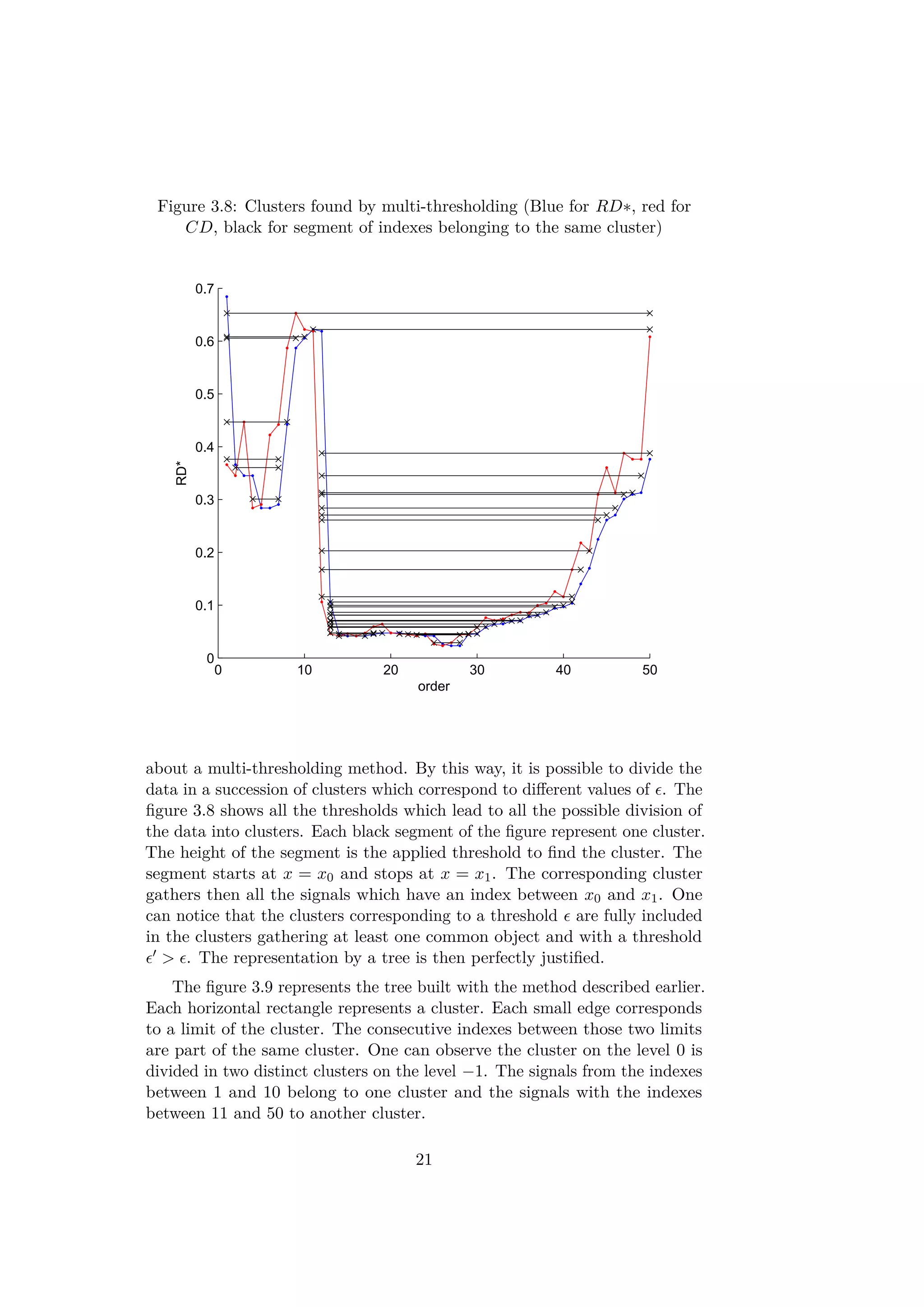
In order to find a hierarchical structure in the database, one can think
20](https://image.slidesharecdn.com/ff3a18c7-0e8d-4852-b4ba-9bdc3c906b26-151031192058-lva1-app6892/75/Thesis_Report-29-2048.jpg)


![Chapter 4
The classification function
After the acquisition of labels by the clustering algorithm and the interaction
of the operator, a classification function can be processed by the algorithm
to automatically detect and classify the failures without extra intervention
from the operator. This part explains then the classification and the learning
method used for the failure detection and classification algorithm.
4.1 Requirements
The proposed classification is created with the data provided after the clus-
tering and the acquisition of labels. Only the data corresponding to the
selected clusters is kept. All the signals considered as noise and too far from
one of the scenarios found are removed. However, even if a set of failures
might have been recorded, a new type of failure could still occur during the
process. The algorithm has to deal with novelty. Moreover, the algorithm
can have to classify between more than two classes of signal. The prob-
lem given here is thus a semi-supervised multi-class machine learning problem.
The detection of a failure for a new signal has to be online. The detection
is part of the real-time process. The response of the algorithm has to be
quick enough to be integrated in the behavior loop. The classification has to
be as accurate as possible in order to avoid some misbehaviors. Finally, the
amount of training data obtained after the clustering is rather small since
the training period must be quite short.
4.2 About semi-supervised multi-class classification
As explained in the article [4], some algorithms used for a two-class clas-
sification can be extended for a multi-class classification. These methods
include among others neural networks, naive Bayes, K-Nearest Neighbor,
27](https://image.slidesharecdn.com/ff3a18c7-0e8d-4852-b4ba-9bdc3c906b26-151031192058-lva1-app6892/75/Thesis_Report-36-2048.jpg)
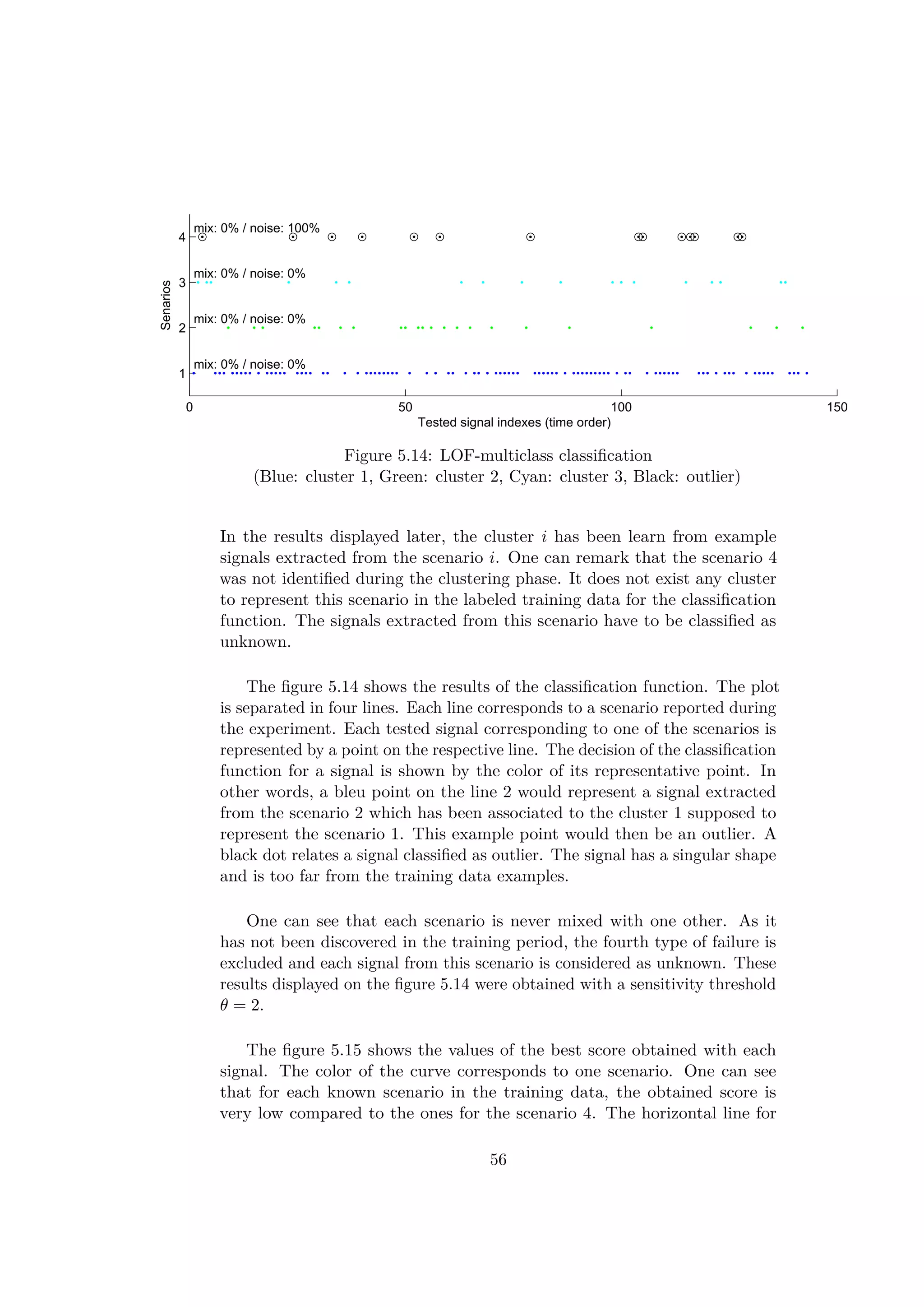
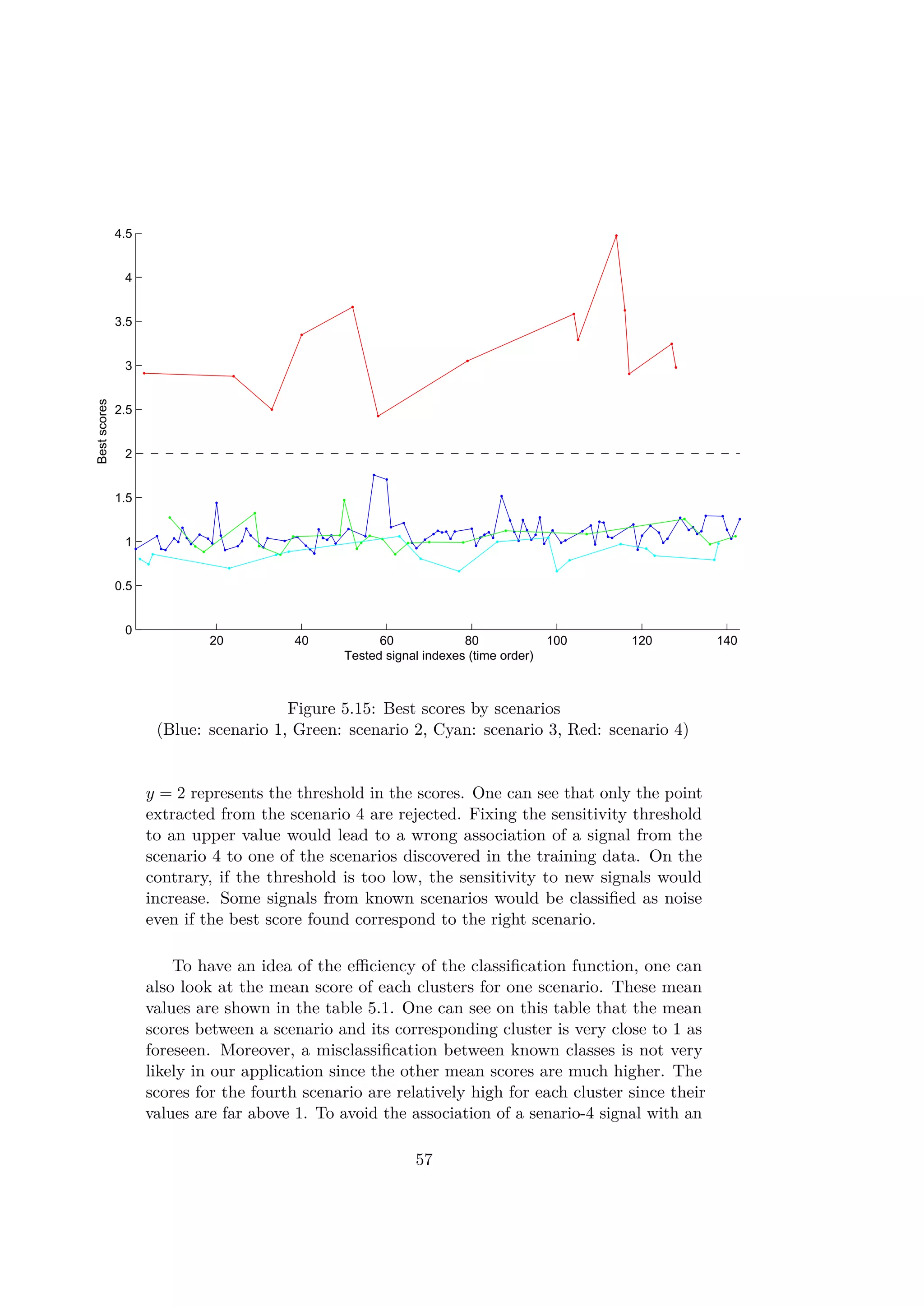
![and support vector machines. However, these algorithms can only classify
between the known classes and cannot detect a novelty.
Another solution is to decompose the problem of multiclass classification
into several binary classification tasks. It exists then two main strategies:
• Strategy One-vs-One
The principle is to define classification functions which compare pairs
of classes. Those classification functions assign a winner class for each
pair. A final vote is done taking into account the winner of each dual.
The class attributed is the one which corresponds to the highest number
of votes
• Strategy One-vs-All
A classification function is created for each class. For each class, the
classification functions answer 1 if the new object belong to their class.
To avoid several classes winning, a score is assigned to each class. The
final classification is done by comparing the scores obtained for each
class and determining the class with the best score.
The strategy one-vs-one is not possible in our case because it is not possible
to detect a possible new failure in a signal. The best strategy is the one-vs-all
because this novelty detection can simply be done by a thresholding on the
score. A too poor score would thus correspond to an outlier. The recorded
signal does not correspond to any known class.
The most standard solution for classification of several classes with the
one-vs-all strategy is the one-class SVM. This solution is however based
on features and representation of the signals in a multi-dimensional space.
As explained in the article [13], the algorithm finds a border which defines
the best the class using Support Vectors implementation. However, the
SVM methods requires a feature description of the objects. One of the most
frequent use case of the algorithm will have to deal with time-series. The
extraction of features being difficult for time-series, this particular method
and all method using feature extraction did not seem suitable for the study
case.
4.3 Local Outlier Factor
The Local Outlier Factor method of (L.O.F) is based on the same principle
as the clustering algorithm used previously. The algorithm uses the density
of the points in the data base to calculate a score (see [7]). Only a distance
function is thus needed to discriminate and classify between the cases. The
28](https://image.slidesharecdn.com/ff3a18c7-0e8d-4852-b4ba-9bdc3c906b26-151031192058-lva1-app6892/75/Thesis_Report-37-2048.jpg)


![5.2 Generic discrimination function for
multi-dimensional time-series
The objects compared by the algorithm are sequences of values mathe-
matically called time-series. Each sensor gives a temporal signal which is
windowed during a critical operation. The information consists of several
synchronous sequences of values from the different sensors. This constitutes
a multidimensional time-series. In order to find a structure or patterns in the
data bases, several techniques are used to distinguish different objects. This
chapter is dedicated to the research of an efficient and generic discrimination
method for time-series and multidimensional time-series.
5.2.1 Related work on time-series
Feature extraction
Many works about machine learning in the literature use feature extraction
to find patterns. A feature is commonly a numerical value which represents
a property of an object. Usually, a feature extraction function can be found
to transform the object into the feature space. Let ω be an object in a set of
objects Ω. One can write the feature extraction function g as:
Ω → Rd
g : ω → x
(5.1)
where x is called the feature vector associated to the object ω.
The use of features allow a vectorial representation of an object in a
d-space, d standing here for the number of features describing the object.
One can thus define borders to create areas in the space corresponding to
one class of object. Intuitively, the learning algorithm creates the borders in
the d-space. Then, the classification function retrieves the domain in which
is the new object is represented by a point.
A large number of studies about pattern recognition for time series have
as well exploited simple features. A common idea is to transform the time
series in the frequency domain by calculating the Discrete Fourier Transform
or to use the Discrete Wavelet Transform. The articles [3] and [18] use this
idea to extract features and classify signals. However to keep the essence
of the information given in the sequence, a lot of frequencies must be kept.
The main problem of such feature extractions is the curse of dimensionality.
As the number of dimensions used to describe an object is high, a large
training set is required to learn efficiently the complex data structure. Some
methods like PCA or other features selection can thus be used to reduce the
42](https://image.slidesharecdn.com/ff3a18c7-0e8d-4852-b4ba-9bdc3c906b26-151031192058-lva1-app6892/75/Thesis_Report-51-2048.jpg)
![dimensionality of the problem in some situations (see [20]). However, those
techniques can hardly be used for novelty detection. By choosing a mixture
of features, a novelty in neglected features could be missed.
Some techniques for feature extraction developed in [9] among others,
consist in finding an ARMA model which fits the behavior of the signal. The
coefficient of the model can be learned and compared. Those features would
describe the signal in a space with far fewer dimensions. Nevertheless, this
approach is more adapted to learn a behavior than a shape of signal. In
our application we are more interested in a temporal change than a general
behavior.
The thesis [19] gives a generic method to extract features from time
signals which describe shapes. Given a set of signals, it divides the time into
segments so that each segment can be represented by one simple behavior.
It can be linear, exponential, triangle, and other shapes. Each feature repre-
sents one parameter of the behavior in a segment. This approach could have
been explored. However, the procedure to calculate the feature seems heavy
and relies on a labeled dataset.
Similarity join
For some kinds of objects like the time-series, it is difficult to define proper
features and to represent them into a d-space. However, it is sometimes easier
to create a similarity function. This function retrieves a positive number,
classically a distance, which evaluates the similarity between two objects.
Let ω1 and ω2 be two objects in Ω. A similarity or distance function f can
be expressed as:
Ω × Ω → R+
f : ω1, ω2 → s
(5.2)
where s is a score evaluating the similarity between ω1 and ω2. This similarity
function is reflexive and positive.
Using the distances between the training data objects and the new un-
classified object, the classification functions find which class of objects the
new object is the most similar to.
A lot of methods used to classify time-series are based on similarity
measurement. Two ubiquitous methods are the Euclidian distance and the
Dynamic Time Warping (or DTW). It consists in evaluating how far the
signals values are in the time-domain. These methods have been explored
and compared in the articles [15, 10] among others. Those distances allow
a comparison of shape between signals by simple mathematical operation.
43](https://image.slidesharecdn.com/ff3a18c7-0e8d-4852-b4ba-9bdc3c906b26-151031192058-lva1-app6892/75/Thesis_Report-52-2048.jpg)
![−5 −4 −3 −2 −1 0 1 2 3 4 5
0
0.2
0.4
0.6
0.8
1
Speed (rad.s
−1
)
pruningfunction
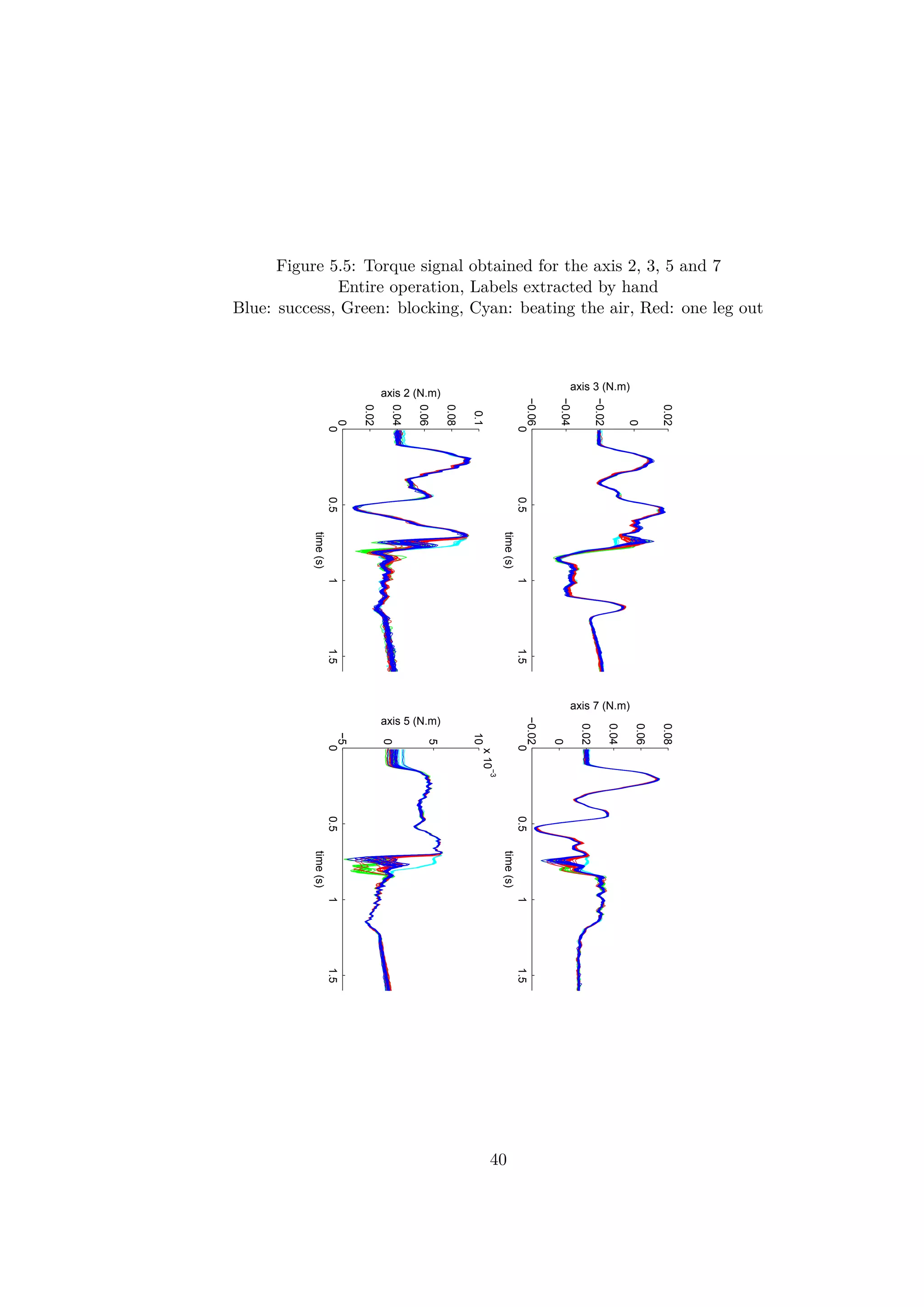
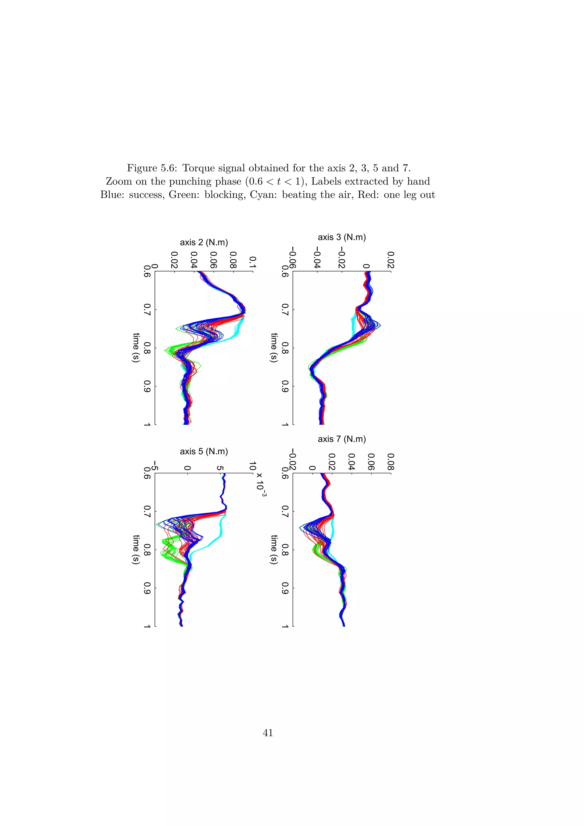
Figure 5.7: Speed pruning function
Instead of including the pruning process in the distance function, a
normalization can be done to produce the same effects as showed in 5.8. The
second step of normalization can be written as in the equation 5.9:
˜xl = Wx
l .ˆxl
where Wx
l = diag([w(xv1
l ), w(xv2
l ), . . . , w(xvK
l )])
(5.9)
The pruning function chosen is a sigmoid function. Its expression is
written in the equation 5.10 and the figure 5.7 represents its shape. The
value of the function is almost zero when the speed is low. When the speed
exceeds a threshold, the function increases and reaches 1. The parameters
has been chosen empirically trying to remove the values corresponding to
the lowest speed and keeping the general shape of the signals (vth = 2 and
λ = 10).
∀v ∈ R, w(v) =
1
1 + exp(−λ(|v| − vth))
(5.10)
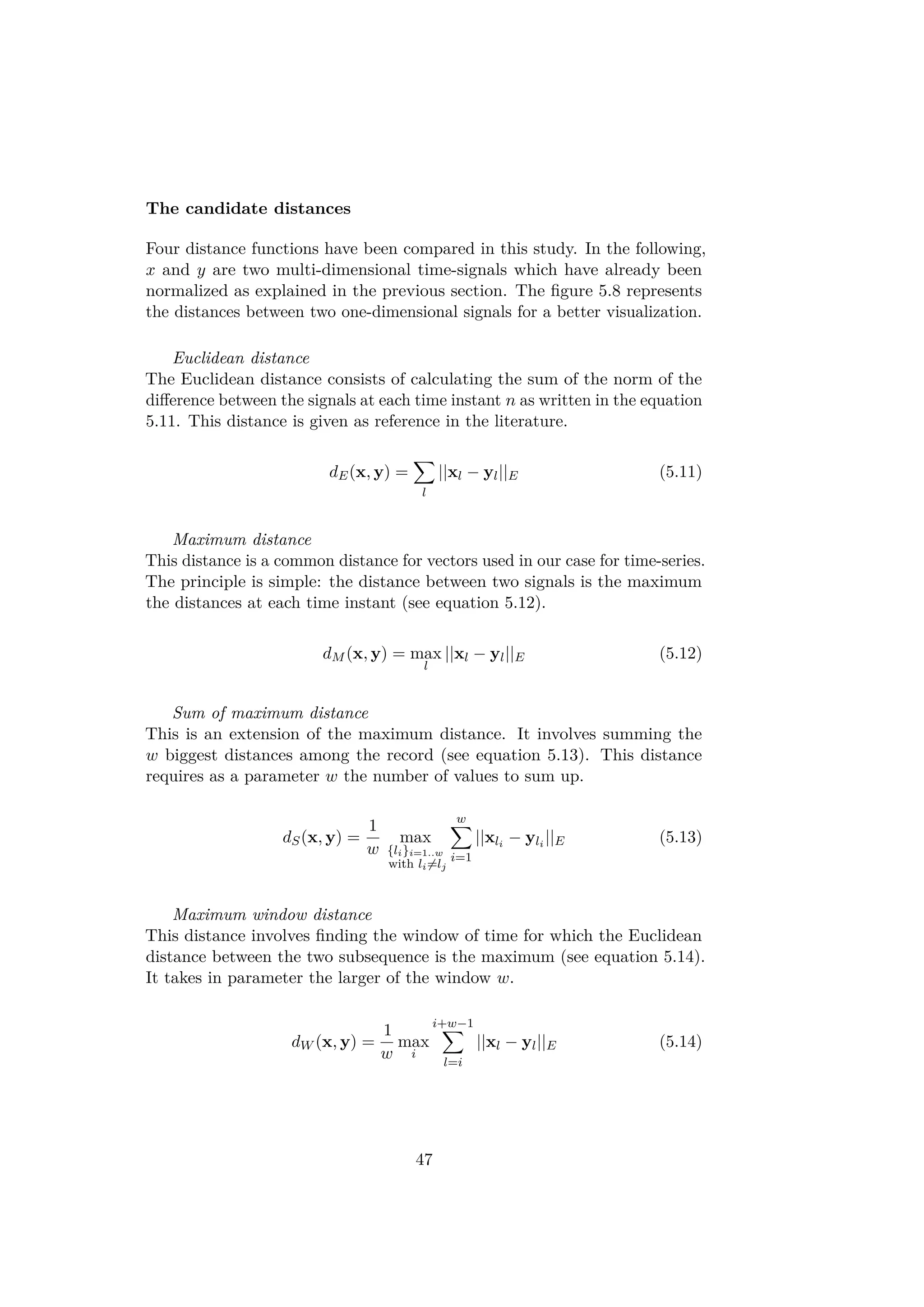
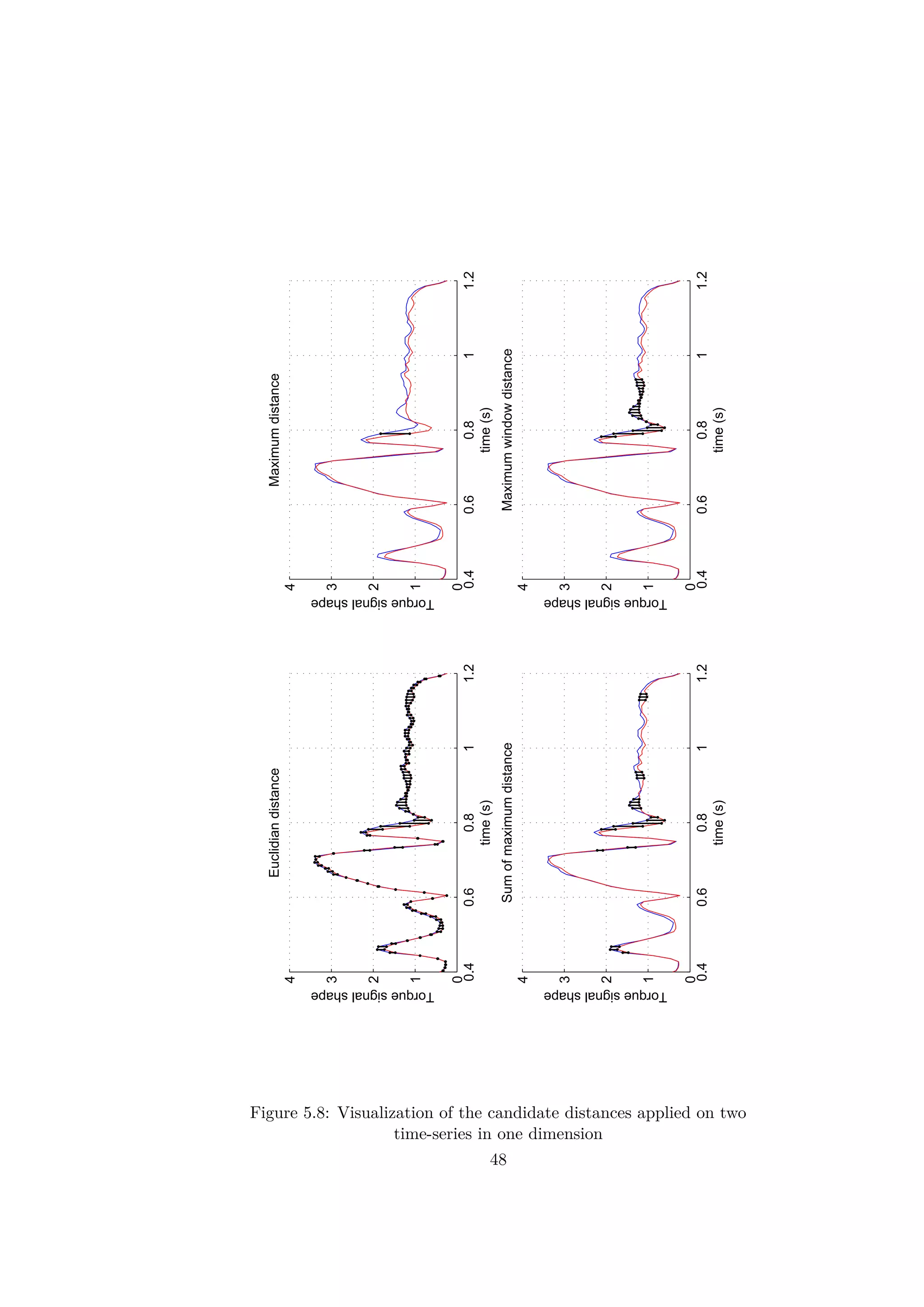
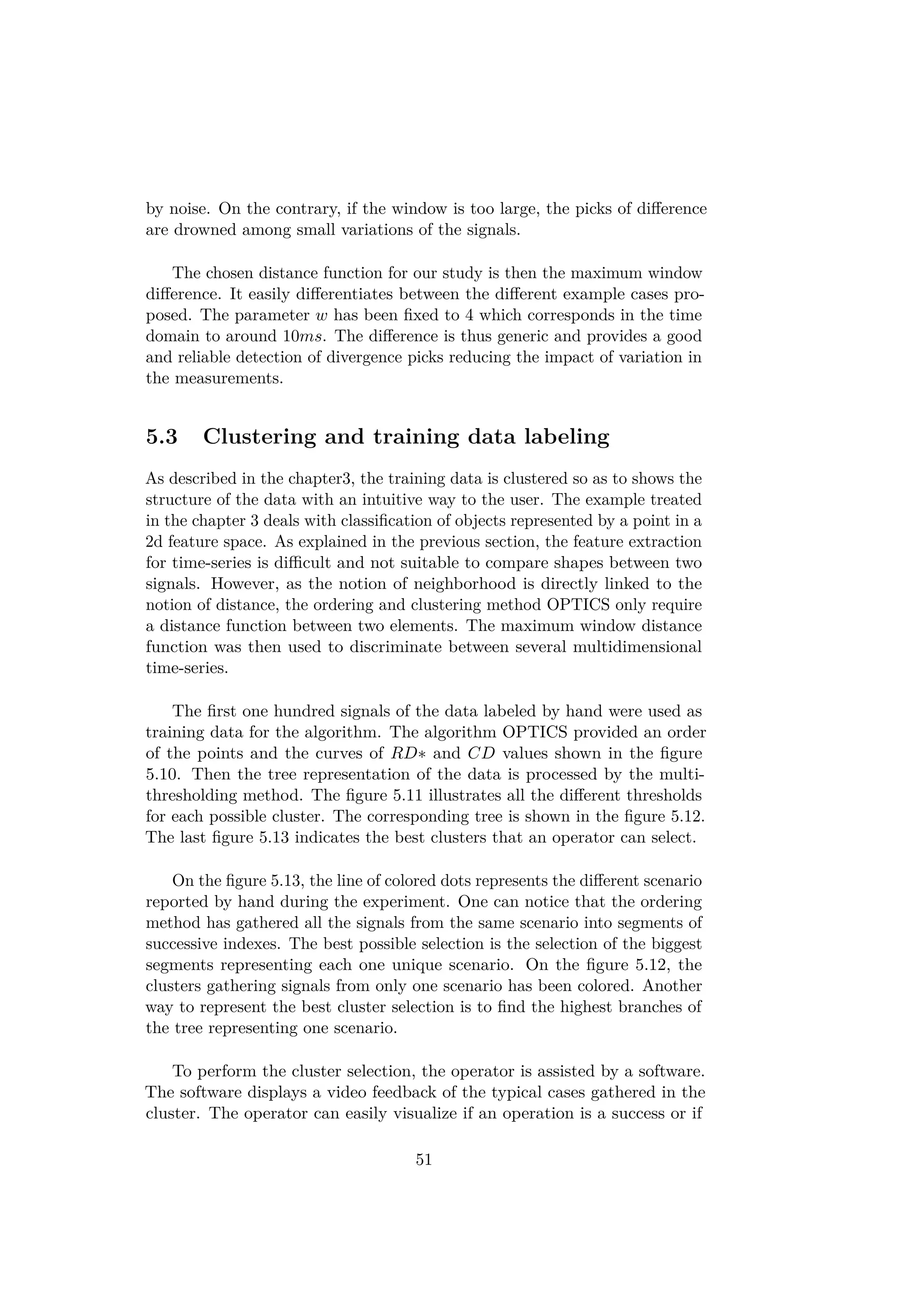
5.2.3 The distance function
To select the most adapted distance function, a comparison between a few
candidates has been made. The distance functions proposed were designed
so as to be simple and adapted for a quick processing. The choice of the
distance function is crucial since it is used to find similarities between the
signals.
46](https://image.slidesharecdn.com/ff3a18c7-0e8d-4852-b4ba-9bdc3c906b26-151031192058-lva1-app6892/75/Thesis_Report-55-2048.jpg)
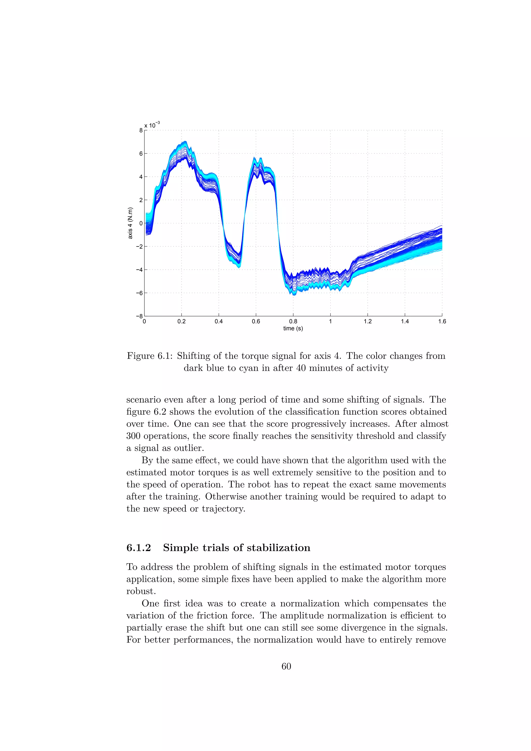
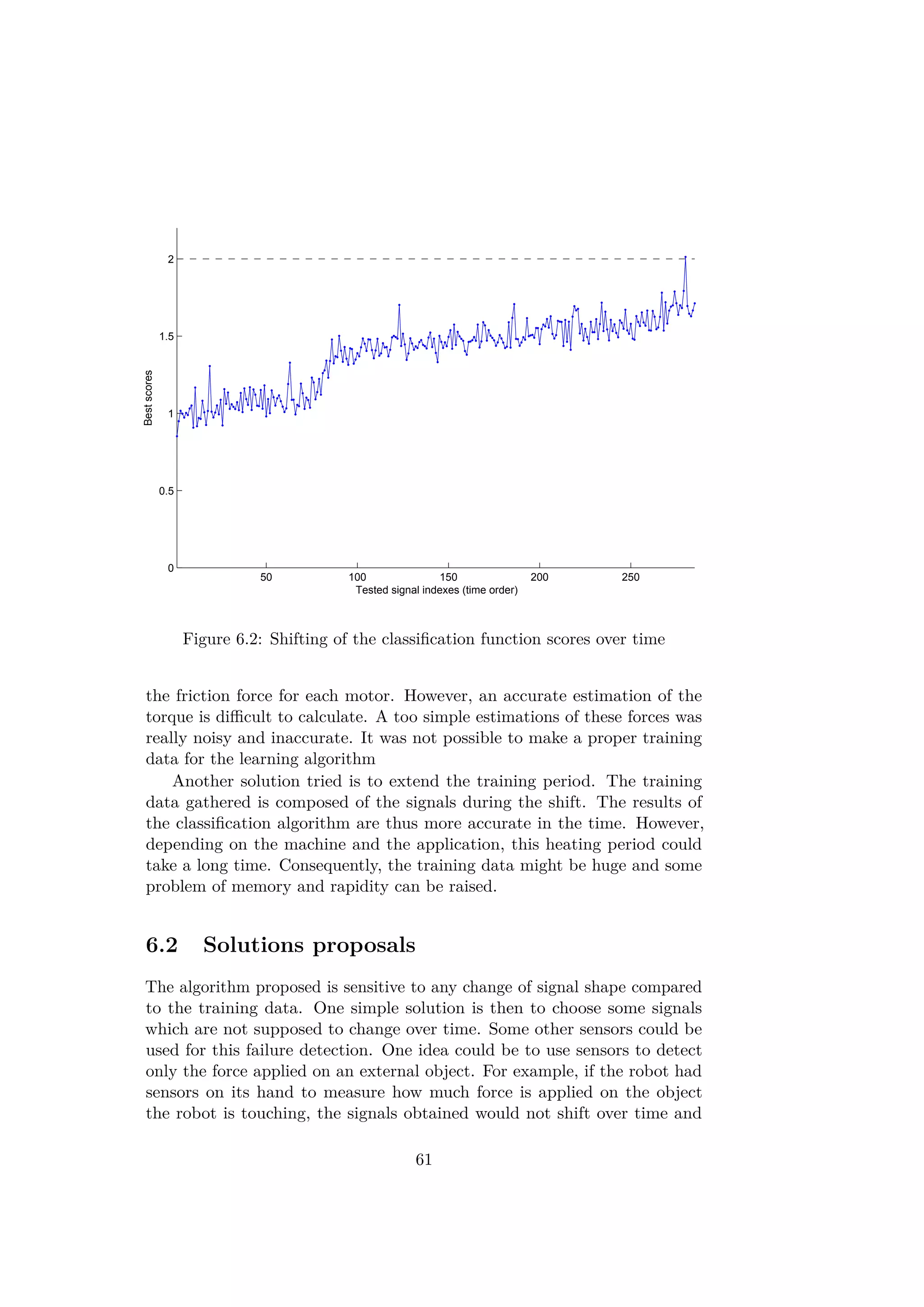
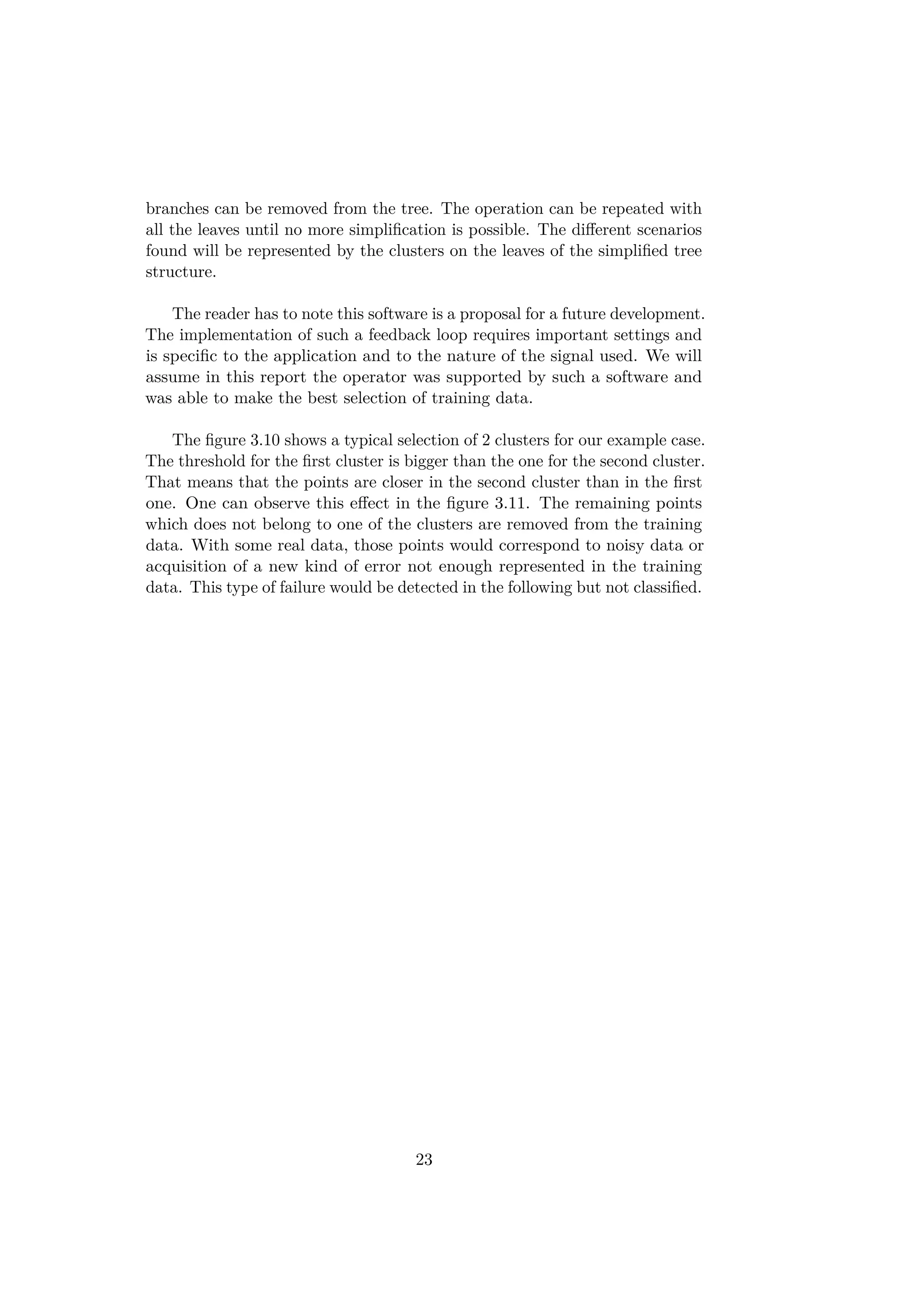
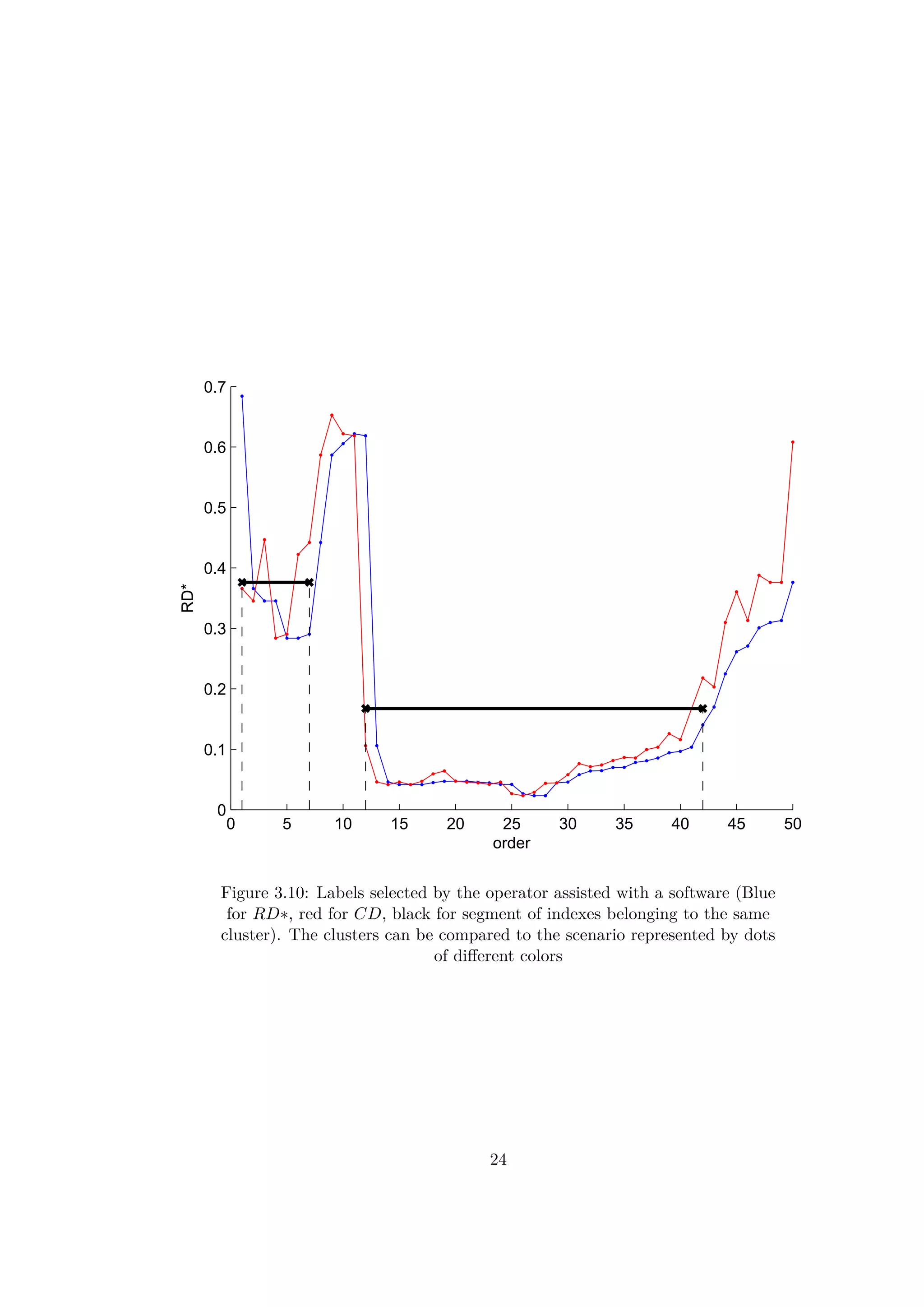
![would have similar patterns attesting the occurrence of a failure. Other
types of sensor can also be used. The operation used in the demo gener-
ates a particular "click" sound once the two parts are correctly assembled.
This sound could be recorded and analyzed in failure detection algorithm.
The sound of the operation is probably stable and would not change over time.
Another way to solve this shifting problem is to improve the machine
learning algorithm to take into account the signal variations. The clustering
algorithm OPTICS has an incremental update version derived in the article
[16]. After the first determination of the success and failures in the RD plot
provided by OPTICS, the algorithm could continuously record and store
new signals and associate them to one of the existing cases. As the shift
occurs in small increments, it could be absorbed in the self-growing training
data. In this manner the classification function could learn the shift. Then
the scenarios could be recognized even after several hours. Nevertheless,
this automatic learning cannot store every single signal for trivial memory
issues. The algorithm would have to choose automatically the most relevant
signals to store or forget some useless signals. Some other issues could as
well appear. For example, two clusters corresponding to different scenarios
could be close to each other and eventually merge together. Such situations
would have to be handled in order to ensure a good general behavior.
One recurrent problem involves the memory required to store the signals.
Indeed the method presented here needs a big quantity of memory to save
the signals encountered in the training period. To decrease the memory
requirements, one can think about a compression of the data which would
decrease the space required. Instead of using the entire signal, only the trend
or the general shape could be used and stored. The signals could be cut
for example in small parts which could be described by a standard behavior
such as linear, constant, exponential... This idea has been explored in the
article [19] to create a complex feature extraction method.
6.3 Similar subjects for further application in ma-
chine learning
Leaving the failure detection aside, this machine learning algorithm could
be used for other applications. It could be used for example to detect an
intrusion in the workspace of the robot: Using proximity sensors placed
on the wrist of the robot, the distance to the object next to the robot
would be recorded during its operation cycle. When someone enters the
robot workspace, the sensors will record a different signal that could be
automatically detected. By the same principle, an impact detection could
be implemented. A collision would generate force signals which diverge
62](https://image.slidesharecdn.com/ff3a18c7-0e8d-4852-b4ba-9bdc3c906b26-151031192058-lva1-app6892/75/Thesis_Report-71-2048.jpg)

![Bibliography
[1] ABB Robotics website. http://new.abb.com/products/robotics/yumi.
[2] Rethink robotics website. http://www.rethinkrobotics.com/.
[3] Rakesh Agrawal, Christos Faloutsos, and Arun Swami. Efficient Simi-
larity Search In Sequence Databases. 1993.
[4] Mohamed Aly. Survey on multiclass classification methods. 2005.
[5] M Ankerst, MM Breunig, HP Kriegel, and J Sander. OPTICS: Oredering
Points To Identify the Clustering Structure. 1999.
[6] J.C. Bezdek. Pattern recognition with fuzzy objective function algo-
rithms. 1987.
[7] Markus M. Breunig, Hans-Peter Kriegel, Raymond T. Ng, and Jörg
Sander. Survey on multiclass classification methods. 2000.
[8] Rodney Brooks. Why we will rely on robots.
http://www.ted.com/talks/rodney_brooks_why_we_will_rely_on_robots,
2013.
[9] Kan Deng, Andrew W. Moore, and Michael C. Nechyba. Learning to
recognize time series: Combining ARMA models with memory-based
learning. 1997.
[10] Alon Efrat, Quanfu Fan, and Suresh Venkatasuramanian. Curve match-
ing, time warping, and light fields: new algorithms for computing
similarity between curves. 2007.
[11] M Ester, Hans-Peter Kriegel, J Sander, and X Xu. A density-based
algorithm for discovering clusters in large spatial databases with noise.
1996.
[12] Sudipto Guha, Rajeev Rastogi, and Kyuseok Shim. Cure: an efficient
clustering algorithm for large databases. 2000.
[13] Chih-Wei Hsu and Chih-Jen Lin. A comparison of methods for multiclass
support vector machines. 2002.
64](https://image.slidesharecdn.com/ff3a18c7-0e8d-4852-b4ba-9bdc3c906b26-151031192058-lva1-app6892/75/Thesis_Report-73-2048.jpg)
![[14] L. Kaufman and P.J. Rousseeuw. Finding groups in data: An introduc-
tion to cluster analysis. 1990.
[15] Eamonn Keogh and Chotirat Ann Ratanamahatana. Exact indexing of
dynamic time warping. 2005.
[16] Hans-Peter Kriegel, Peer Kröger, and Irina Gotlibovich. Incremental
OPTICS: Efficient computation of updates in a hierarchical cluster
ordering. 2003.
[17] J. MacQueen. Some methods for classification and analysis of multi-
variate observations. 1967.
[18] Fabian Mörchen. Time series feature extraction for data mining using
DWT and DFT. 2003.
[19] Robert T. Olszewski. Generalized feature extraction for structural
pattern recognition in time-series data, 2001.
[20] Kiyoung Yang and Cyrus Shahabi. A PCA-based similarity measure for
multivariate time series. 2004.
65](https://image.slidesharecdn.com/ff3a18c7-0e8d-4852-b4ba-9bdc3c906b26-151031192058-lva1-app6892/75/Thesis_Report-74-2048.jpg)