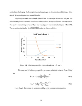
This document is a thesis submitted by Jorge Andres Navas Guzman, Sr. to the University of Texas at Austin for the degree of Master of Science in Engineering. The thesis focuses on simulating chemical enhanced oil recovery, specifically polymer flooding and surfactant polymer flooding, in a highly stratified and heterogeneous oil reservoir in Colombia. The objectives are to evaluate different scenarios of polymer flooding and surfactant polymer flooding in producer layers A and B and provide recommendations to improve oil recovery in the field. A sector model was constructed from a commercial reservoir simulator and history matched. Simulation results show that polymer flooding in layer A can increase oil recovery by up to 12% compared to waterflooding alone. Extending polymer flooding to layer


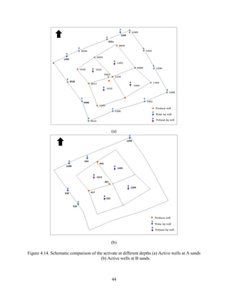
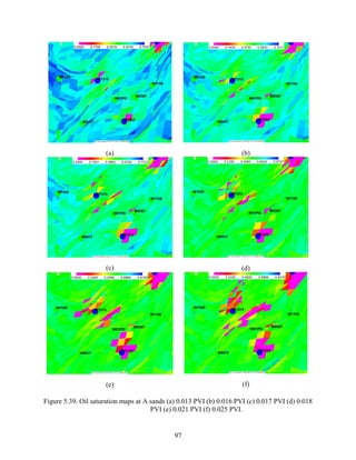
![52
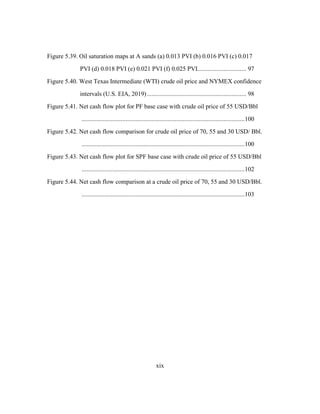
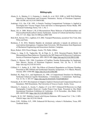
as an interpolation between the pure oil and water parameters based on the oil volume fraction in
the microemulsion phase. Therefore, the relative permeabilities model is used in this work:
( )
c c
= − +
3 23 1 23 2
1
, (4.27)
where the parameter Ψ is any of the following:
,high
r
k0
3 ,
,low
r
k0
3 ,
high
n3 ,
low
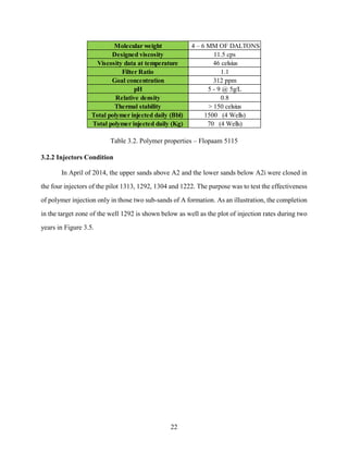
n3 ,
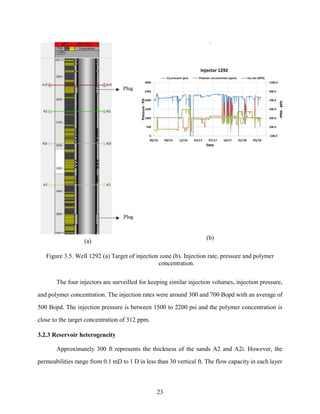
high
r
S 3 ,
low
r
S 3 , and T3
, where
,high
r
k0
3 is the microemulsion relative permeability endpoint at high trapping number,
,low
r
k0
3 is the
microemulsion relative permeability endpoint at low trapping number,
high
n3 is the microemulsion
relative permeability exponent at high trapping number,
low
n3 is the microemulsion relative
permeability exponent at low trapping number,
high
r
S 3 is the microemulsion relative permeability
residual saturation at high trapping number, and
low
r
S 3 is the microemulsion relative permeability
residual saturation at high trapping number.
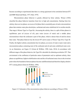
Phase Behavior Model
Effective Salinity
The effective salinity model mentioned in UTCHEMRS (2017) is represented by the next
equation:
𝐶𝑆𝐸 = 𝐶51(1 − 𝛽6𝑓6
𝑠)−1
(1 + 𝛽𝑇(𝑇 − 𝑇𝑟𝑒𝑓))
−1
(4.28)
where 𝐶51is the aqueous phase anion concentration; 𝛽6 is a positive constant; 𝑓6
𝑠
=
𝐶6
𝑠
𝐶3
𝑚 is the
fraction of the divalent cations bound to surfactant micelles; and 𝛽𝑇 is the temperature coefficient.
Binodal Curve
The phase behavior for microemulsion systems can be modelled using the extended Hand’s
rule (Pope and Nelson, 1978). The extended Hand’s rule considers the following relationship for
the binodal curves:
𝐶3𝑙
𝐶2𝑙
= 𝐴 (
𝐶3𝑙
𝐶1𝑙
)
𝐵
𝑓𝑜𝑟 𝑙 = 1,2 𝑜𝑟 3
(4.29)
the constraints for the phase compositions are
, ,..., p
c c c n
+ + = =
1 2 3 1 1 (4.30)
and B=-1 for symmetric binodal curves, 𝐶3𝑙 is denotes as
𝐶3𝑙 =
1
2
[−𝐴𝐶2𝑙 + √(𝐴𝐶2𝑙)2 + 4𝐴𝐶2𝑙(1 − 𝐶2𝑙)] 𝑓𝑜𝑟 𝑙 = 1,2 𝑜𝑟 3 (4.31)](https://image.slidesharecdn.com/thesis19navas-220523220444-9860e2a3/85/thesis19navas-pdf-71-320.jpg)


![Heinemann zoltán e[1]._-_petroleum_recovery_](https://cdn.slidesharecdn.com/ss_thumbnails/heinemannzoltne1-150111210400-conversion-gate02-thumbnail.jpg?width=640&height=640&fit=bounds)

![Heinemann zoltán e[1]._-_petroleum_recovery_](https://cdn.slidesharecdn.com/ss_thumbnails/heinemannzoltne1-150111211406-conversion-gate02-thumbnail.jpg?width=640&height=640&fit=bounds)


