2. 162 II. Sharp inequalities
s n
s= +1
p
n
1 s=
p
1
s=n −1
p
1 1
1
r p
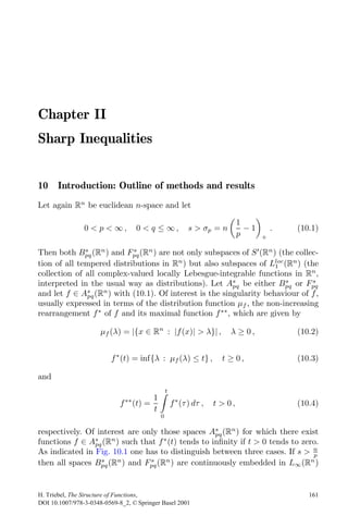
Fig. 10.1
and, hence, all functions f ∗ (t) with f ∈ As (Rn ) are bounded. This is of no
pq
interest for us (at least as far as only the growth of functions is considered).
The two remaining cases are called:
n
sub-critical if 0 < p < ∞ , 0 < q ≤ ∞ , σp < s < , (10.5)
p
and
n
critical if 0 < p < ∞ , 0 < q ≤ ∞, s= . (10.6)
p
In all spaces belonging to the sub-critical case there are essentially unbounded
functions f with f ∗ (t) → ∞ if t ↓ 0. In the critical case the situation is more
delicate. It depends on the parameters p, q and whether As is Bpq or Fpq . We
pq
s s
give in Section 11 a detailed and definitive description of the relevant scenery
surrounding the embedding of the spaces Bpq (Rn ) and Fpq (Rn ) in Lloc (Rn ),
s s
1
n s n
L∞ (R ) and other classical target spaces. Let Apq (R ) be a space which is
embedded in Lloc (Rn ) but not in L∞ (Rn ). Then (in temporarily somewhat
1
vague terms) the growth envelope function EG As is a function t → EG As (t)
pq pq
which is equivalent to
EG |As (t) = sup f ∗ (t) :
pq f |As (Rn ) ≤ 1 ,
pq 0 < t < ε, (10.7)
3. 10. Introduction: Outline of methods and results 163
where 0 < ε < 1 is a given number. The notation EG |As indicates that this
pq
function is taken with respect to a given quasi-norm · |As (Rn ) . If
pq
· |As (Rn )
pq 1 ∼ · |As (Rn )
pq 2 (10.8)
are two equivalent quasi-norms in a given space As (Rn ), then (in obvious
pq
notation)
EG |1 As (t) ∼ EG |2 As (t) ,
pq pq 0 < t ≤ ε, (10.9)
are also equivalent. Since we never distinguish between equivalent quasi-norms
of a given space As (Rn ) it is reasonable to extend this point of view to what
pq
we wish to call later on the growth envelope function EG As . By definition one
pq
has the sharp inequality
f ∗ (t)
sup ≤ c f |As (Rn ) , f ∈ As (Rn ) . (10.10)
0<t<ε EG |As (t)
pq
pq pq
One may look at the left-hand side of (10.10) as the quasi-norm L∞ (Iε , μ) for
a suitable Borel measure μ on the interval Iε = (0, ε]. We wish to strengthen
(10.10), replacing L∞ (Iε , μ) by Lu (Iε , μ). Let EG (t) be an unbounded positive,
continuous, monotonically decreasing function on Iε (this will apply in par-
ticular to all growth envelope functions with which we deal later on). Then
the associated Borel measure μ = μΨ with respect to the distribution function
Ψ(t) = − log EG (t) is the natural and distinguished choice for the above pur-
pose. If g(t) is a non-negative monotonically decreasing function on Iε (with
g = f ∗ where f ∈ As (Rn ) as a typical example) then the corresponding
pq
quasi-norms are monotone,
⎛ ε ⎞ u1
u1 1
g(t) ⎝ g(t) ⎠
sup ≤ c1 μΨ (dt)
0<t<ε EG (t) EG (t)
0
⎛ ε
⎞ u1
u0 0
g(t)
≤ c0 ⎝ μΨ (dt)⎠ , (10.11)
EG (t)
0
where 0 < u0 < u1 < ∞. We refer to Proposition 12.2. Hence by (10.10) it
makes sense to ask for the smallest number u = u(As ) with 0 < u ≤ ∞ such
pq
that
⎛ ε ⎞u1
∗ u
⎝ f (t)
μΨ (dt)⎠ ≤ c f |As (Rn ) , f ∈ As (Rn ) , (10.12)
EG (t) pq pq
0
where
EG (t) = EG As (t) and Ψ(t) = − log EG As (t) .
pq pq
4. 164 II. Sharp inequalities
We denote provisionally the couple
EG (As ) = EG As (t), u
pq pq (10.13)
as the growth envelope of As (Rn ). We calculate the growth envelopes for all
pq
relevant spaces with the typical outcome
1
EG (As ) = (t− r , u) and EG (As ) = (| log t|v , u)
pq pq (10.14)
in the sub-critical and critical case, respectively. Here r has the same meaning
as in Fig. 10.1, whereas 0 < u ≤ ∞ and 0 < v ≤ 1 are suitable numbers
s s
depending on the parameters in Bpq and Fpq . In particular, the growth en-
velope exists in all cases. It is a natural and very precise description of the
growth of functions belonging to As (Rn ). Inserting (10.14) in (10.12) one gets
pq
quasi-norms of the same type as in the Lorentz spaces Lru (Iε ) or in the special
Lorentz-Zygmund spaces L∞,u (log L)a (Iε ). However in the above outlined con-
text neither spaces of this nor any other type are prescribed as target spaces in
the course of setting up the required inequalities, and asking only afterwards
for best parameters. (Of course all the spaces Lru (log L)a (Iε ) are reasonable
refinements of classical target spaces like Lp , C, etc.) Here they emerge natu-
rally and, hence, they are at the heart of the matter of the described singularity
theory.
If s > n then all spaces As (Rn ) are embedded in L∞ (Rn ) and a singularity
p pq
theory in the above argument does not make much sense. However in the
context of continuity there is one case which has attracted special attention in
recent times and which corresponds to the line s = 1 + n in Fig. 10.1. Hence
p
we complement (10.5) and (10.6) by the case called:
n
super-critical if 0 < p < ∞ , 0 < q ≤ ∞, s=1+ . (10.15)
p
First we recall that
ω(f, t)
ω(f, t) = sup |f (x + h) − f (x)| and ω(f, t) = (10.16)
x∈Rn ,|h|≤t t
with t > 0, are the usual modulus of continuity and the divided modulus of
continuity, respectively. Then Lip(Rn ) is the collection of all complex-valued
functions in Rn such that
f |Lip(Rn ) = sup |f (x)| + sup ω(f, t) < ∞ . (10.17)
x∈Rn 0<t<1
We have the remarkable fact (explained in greater detail in Section 11) that
n
1+ n
Apq (Rn ) ⊂ L∞ (Rn ) if, and only if, Apq p (Rn ) ⊂ Lip(Rn ) .
p
(10.18)
5. 10. Introduction: Outline of methods and results 165
This makes (almost) clear that in the critical case (10.6) the growth envelope
n
function EG Apq is unbounded if, and only if, the continuity envelope function
p
1+ n
EC Apq p , defined as an equivalent function to
1+ n 1+ n
EC |Apq p (t) = sup ω(f, t) : f |Apq p (Rn ) ≤ 1 , 0 < t < ε, (10.19)
for some ε > 0, is unbounded. Obviously, we rely here on the same nota-
tional agreement as in connection with (10.7), (10.8), (10.9). Furthermore, up
to equivalences, the continuity envelope function is positive, continuous and
monotonically decreasing in the interval (0, ε]. Then one has an immediate
counterpart of (10.11), (10.12), which justifies the introduction of the continu-
ity envelope
1+ n 1+ n
EC (Apq p ) = EC Apq p (t), u (10.20)
in analogy to (10.13). We feel that the outcome is beautiful and perfect: One
has in all cases of interest, this means all cases not covered by (10.18),
n
1+ n
EG (Apq ) = EC (Apq p ) .
p
(10.21)
We shall deal first with the critical case and afterwards lift not only the in-
equalities but also some extremal functions, responsible for the sharpness, by
1 to the super-critical case. In the one-dimensional case this is based on the
simple but rather effective observation,
ω(f, t) ≤ c |f |∗∗ (t) , 0 < t < 1, (10.22)
which provides at least an understanding of the method. (We use the notation
introduced in (10.4)). There is a counterpart in Rn , but it is more complicated.
It may be found in 12.16.
The close connection between inequalities of Hardy type and rearrangement
inequalities hidden in (10.12), (10.14), is based on the well-known observation,
∞
b (x) |f (x)| dx ≤
p p
b∗p (t) f ∗p (t) dt , 0 < p < ∞, (10.23)
Rn
0
where b(x) is a non-negative compactly supported weight function. This ap-
proach to Hardy inequalities has the advantage that both the singularity be-
haviour of the fixed weight function b(x) and also of f , belonging to a given
function space, are considered on a global scale. In particular, b(x) may degen-
erate not only in points, hyper-planes, or smooth surfaces, but also on rather
6. 166 II. Sharp inequalities
irregular sets. Let, as an example, Γ be a compact d-set in Rn according to
(9.67) with 0 < d < n, and let
D(x) = dist (x, Γ) , x ∈ Rn , (10.24)
be the distance of x ∈ Rn to Γ. Then
b(x) = D(x)a | log D(x)|b , a < 0, b ∈ R, 0 < D(x) < 1 , (10.25)
is a typical weight function in our context. One obtains, for example, in the
n
critical case (10.6) for spaces Fpq (Rn ) not covered by (10.18) (this means
p
1 < p < ∞) the Hardy inequality
p
f (x) dx n
≤ c f |Fpq (Rn )
p p
(10.26)
log D(x) Dn−d (x)
D(x)<ε
where 0 < ε < 1 and 0 < q ≤ ∞. Recall that this applies in particular to the
Sobolev spaces
n n
Hpp (Rn ) = Fp,2 (Rn ) ,
p
1 < p < ∞. (10.27)
If d = 0, then one may choose Γ = {0} and gets
p
f (x) dx n
≤ c f |Fpq (Rn )
p p
, 1 < p < ∞, (10.28)
log |x| |x|n
|x|<ε
0 < q ≤ ∞, 0 < ε < 1, where again (10.27) is an outstanding example.
The indicated approach, which means the reduction of Hardy inequalities via
(10.23) to rearrangement inequalities, is universal in our context. In particular
it applies to all sub-critical cases and those critical cases which are not covered
by (10.18). However the outcome is not always satisfactory. There seems to be
a tricky interplay between weights, the geometry of Γ, and possible measures
on Γ. We will discuss this point later on, although there are no final answers.
For example, (10.26) looks better than it really is. On the other hand in case of
Γ = {0} one gets sharp assertions: The functions responsible for the sharpness
of the rearrangement inequalities are also extremal functions for the related
Hardy inequalities. Roughly speaking, these extremal functions convert the
inequality (10.23) into an equivalence.
This chapter is organized as follows. In Section 11 we set the scene and collect
(mostly without proofs) a few well-known classical embedding assertions in
all three cases. Section 12 deals both with growth and continuity envelopes.
Here we rely, at least partly, on recent work of D. D. Haroske, [Har01], where
7. 11. Classical inequalities 167
she introduced the notation of envelopes used above and studied growth and
continuity envelopes systematically and, in particular, in the context of more
general spaces. We restrict ourselves here to those properties which are more
or less of direct use for later applications to the spaces Bpq (Rn ) and Fpq (Rn ).
s s
On this basis we study in Sections 13, 14 and 15 the critical, super-critical
and sub-critical case, respectively. Hardy inequalities in the setting outlined
above, will be considered in Section 16. Finally we collect in Section 17 some
additional material and references.
11 Classical inequalities
11.1 Some notation
We use the notation introduced in the previous sections. In particular, let Rn
be again euclidean n-space where n ∈ N. The Schwartz space S(Rn ), its dual
S (Rn ), and the spaces Lp (Rn ) with 0 < p ≤ ∞ have the same meaning as
in 2.1, the latter quasi-normed by (2.1). Let Lloc (Rn ) be the collection of all
1
complex-valued locally Lebesgue-integrable functions in Rn . Any f ∈ Lloc (Rn )
1
is interpreted in the usual way as a regular distribution. Conversely, as usual,
a distribution on Rn is called regular if, and only if, it can be identified (as a
distribution) with a locally integrable function on Rn . If A(Rn ) is a collection
of distributions on Rn , then
A(Rn ) ⊂ Lloc (Rn )
1 (11.1)
simply means that any element f of A(Rn ) is a regular distribution f ∈
Lloc (Rn ). Then, in particular, the distribution function μf (λ), the rearrange-
1
ment f ∗ (t) and its maximal function f ∗∗ (t) in (10.2)–(10.4) make sense accept-
ing that they might be infinite. If A1 (Rn ) and A2 (Rn ) are two quasi-normed
spaces, continuously embedded in S (Rn ), then
A1 (Rn ) ⊂ A2 (Rn ) (11.2)
always means that there is a constant c > 0 such that
f |A2 (Rn ) ≤ c f |A1 (Rn ) for all f ∈ A1 (Rn ) , (11.3)
(continuous embedding). On the other hand we do not use the word embedding
in connection with inequalities of type (10.12).
The spaces Bpq (Rn ) and Fpq (Rn ) for the full scale of parameters
s s
0 < p ≤ ∞, 0 < q ≤ ∞, s ∈ R, (11.4)
8. 168 II. Sharp inequalities
(with p < ∞ in the F -case) were introduced in Definitions 2.6 and 3.4 or in a
more traditional (this means Fourier-analytical) way in connection with The-
orems 2.9 and 3.6. A list of special cases, including Sobolev spaces, classical
Sobolev spaces, H¨lder-Zygmund spaces, and classical Besov spaces, may be
o
found in 1.2. Although they are not special cases of the two scales Bpq (Rn )
s
and Fpq (Rn ) we need also the spaces C(Rn ), C 1 (Rn ), and Lip(Rn ). The latter
s
space, including the modulus of continuity and the divided modulus of conti-
nuity were introduced in (10.17) and (10.16), respectively. Recall that C(Rn )
is the space of all complex-valued, bounded, uniformly continuous functions in
Rn , normed by
f |C(Rn ) = sup |f (x)| , (11.5)
x∈Rn
whereas
∂f
C 1 (Rn ) = f ∈ C(Rn ) : ∈ C(Rn ) with j = 1, . . . , n (11.6)
∂xj
is the obviously normed related space of differentiable functions. Then C 1 (Rn )
is a closed subspace of Lip(Rn ) and by the mean value theorem,
f |C 1 (Rn ) ∼ f |Lip(Rn ) , f ∈ C 1 (Rn ) , (11.7)
(equivalent norms). First we clarify under what conditions Bpq (Rn ) and
s
s n
Fpq (R ) consist of regular distributions according to (11.1).
The word classical in the heading of this Section 11 has a double meaning. In
Theorems 11.2 and 11.4 we collect (mainly without proofs) sharp embeddings
in classical target spaces such as
Lloc (Rn ) ,
1 Lr (Rn ) , C(Rn ) , C 1 (Rn ) , Lip(Rn ) ,
whereas Theorem 11.7 describes those classical refined inequalities in limiting
situations (from the middle of the 1960s up to around 1980) which are the
roots of recent research and, in particular, of our further intentions in this
chapter.
11.2 Theorem
(i) Let
0 < p < ∞, 0 < q ≤ ∞, s ∈ R. (11.8)
Then
Fpq (Rn ) ⊂ Lloc (Rn )
s
1 (11.9)
9. 11. Classical inequalities 169
if, and only if,
1
either 0 < p < 1, s≥n −1 , 0 < q ≤ ∞, (11.10)
p
or 1 ≤ p < ∞, s > 0, 0 < q ≤ ∞, (11.11)
or 1 ≤ p < ∞, s = 0, 0 < q ≤ 2. (11.12)
(ii) Let
0 < p ≤ ∞, 0 < q ≤ ∞, s ∈ R. (11.13)
Then
Bpq (Rn ) ⊂ Lloc (Rn )
s
1 (11.14)
if, and only if,
1
either 0 < p ≤ ∞, s>n −1 , 0 < q ≤ ∞, (11.15)
p +
1
or 0 < p ≤ 1, s=n − 1 , 0 < q ≤ 1, (11.16)
p
or 1 < p ≤ ∞, s = 0 , 0 < q ≤ min(p, 2) . (11.17)
11.3 Remark
This theorem coincides with Theorem 3.3.2 in [SiT95], where one finds also
a proof. We refer also to [RuS96], pp. 32–35, where some of the key ideas of
the proof are outlined. This theorem clarifies in a final way for which spaces
Fpq (Rn ) and Bpq (Rn ) it makes sense to look at the distribution function μf (λ)
s s
in (10.2) and at the rearrangement f ∗ (t) in (10.3) and to ask the questions
sketched in the introduction in Section 10. We restrict ourselves in the sequel
to spaces Bpq (Rn ) and Fpq (Rn ) with (10.1). In other words we exclude all
s s
1
borderline cases covered by Theorem 11.2 where either p = ∞ or s = n( p −1)+ .
It would be of interest to have a closer look at these excluded spaces and also
at a few other spaces not treated here, for example F∞q (Rn ), including in
s
particular bmo(Rn ). Later on we return to these excluded spaces and add in
13.7 some comments and give a few references.
Next we wish to clarify the embedding of the spaces Bpq (Rn ) and Fpq (Rn ) in
s s
the sub-critical, critical, super-critical case, according to (10.5), (10.6), (10.15),
respectively, in distinguished target spaces; this means Lr (Rn ) in the sub-
critical case (where r has the same meaning as in Fig.10.1), L∞ (Rn ) and C(Rn )
in the critical case, Lip(Rn ) and C 1 (Rn ) in the super-critical case. These are
10. 170 II. Sharp inequalities
the only cases of interest for us in the context outlined in Section 10. We do
not repeat other assertions of the substantial embedding theory of the spaces
Bpq (Rn ) and Fpq (Rn ), including their special cases as Sobolev and H¨lder-
s s
o
Zygmund spaces. The classical part of this theory may be found in [Triα],
2.8, and the almost classical part in [Triβ], 2.7.1. The final clarification of this
type of embeddings goes back to [SiT95]. Descriptions of these results may
be found in [RuS96], 2.2 and in [ET96], 2.3.3. As said, we restrict ourselves
here to those special assertions which are directly related to the problems
outlined in Section 10. Recall that the spaces C(Rn ), C 1 (Rn ), and Lip(Rn )
were introduced in 11.1 and (10.17).
11.4 Theorem
(i) (Sub-critical case) Let
n n
1 < r < ∞, s > 0, s− =− , and 0 < q ≤ ∞ , (11.18)
p r
(the dashed line in Fig. 10.1). Then
Bpq (Rn ) ⊂ Lr (Rn ) if, and only if, 0 < q ≤ r ,
s
(11.19)
and
Fpq (Rn ) ⊂ Lr (Rn ) for all
s
0 < q ≤ ∞. (11.20)
(ii) (Critical case) Let
n
0 < p < ∞, 0 < q ≤ ∞, s= . (11.21)
p
Then
n
Bpq (Rn ) ⊂ C(Rn ) if, and only if, 0 < p < ∞ ,
p
0 < q ≤ 1, (11.22)
and
n
Fpq (Rn ) ⊂ C(Rn ) if, and only if, 0 < p ≤ 1 ,
p
0 < q ≤ ∞. (11.23)
In (11.22) and (11.23) one can replace C(Rn ) by L∞ (Rn ).
(iii) (Super-critical case) Let
n
0 < p < ∞, 0 < q ≤ ∞, s=1+ , (11.24)
p
11. 11. Classical inequalities 171
(the dotted line in Fig. 10.1). Then
1+ n
Bpq p
(Rn ) ⊂ C 1 (Rn ) if, and only if, 0 < p < ∞ , 0 < q ≤ 1, (11.25)
and
1+ n
Fpq p
(Rn ) ⊂ C 1 (Rn ) if, and only if, 0 < p ≤ 1 , 0 < q ≤ ∞. (11.26)
In (11.25) and (11.26) one can replace C 1 (Rn ) by Lip(Rn ).
Proof (of part (iii)) Detailed proofs of parts (i) and (ii) may be found in
[SiT95], Theorems 3.2.1 and 3.3.1, Remark 3.3.5; short descriptions are given
in [RuS96], 2.2, and in [ET96], 2.3.3. Part (iii) is essentially the lifting of part
(ii) by 1. But this is by no means obvious and must be justified. First we
remark that
1+ n n
∂f n
f ∈ Fpq p
(Rn ) if, and only if, f ∈ Fpq (Rn ) and
p
∈ Fpq (Rn )
p
∂xj
(11.27)
where j = 1, . . . , n and (equivalent quasi-norms)
n
1+ n n
∂f n
f |Fpq p (Rn ) ∼ f |Fpq (R ) +
p n
|Fpq (Rn ) .
p
(11.28)
j=1
∂xj
We refer to [Triβ], Theorem 2.3.8, pp. 58/59. Hence, the if-part of (11.26)
follows from (11.23). Conversely, assume
1+ n
Fpq p
(Rn ) ⊂ C 1 (Rn ) for some 0 < p < ∞ , 0 < q ≤ ∞. (11.29)
We construct special Fourier multipliers and introduce some cones in Rn ,
Kt = {ξ = (ξ , ξn ) ∈ Rn : ξn > 0 , |ξ | < tξn } , t > 0, (11.30)
where obviously ξ = (ξ1 , . . . , ξn−1 ) ∈ Rn−1 . Let ϕ be a C ∞ function in Rn {0}
with
ξ
ϕ(ξ) = ϕ , ϕ(ξ) = 1 if ξ ∈ Kt and supp ϕ ⊂ K2t . (11.31)
|ξ|
Let ψ(ξ) be a C ∞ function in Rn which is identically 1 if |ξ| ≥ 1 and 0 ∈ supp ψ.
Then, by [Triβ], Theorem 2.3.7 on p. 57,
−1
ϕj (ξ) = ϕ(ξ) ψ(ξ) ξj ξn , where j = 1, . . . , n , (11.32)
12. 172 II. Sharp inequalities
are Fourier multipliers in all spaces Fpq (Rn ) and Bpq (Rn ). Let
s s
n
f ∈ Fpq (Rn ) with supp f ⊂ Kt ∩ {ξ ∈ Rn : |ξ| > 1} ,
p
(11.33)
and
∨ ∨
−1 −1
g(x) = ξn f (ξ) (x) = ξn ϕn (ξ) f(ξ) (x) , x ∈ Rn , (11.34)
where we used the notation introduced in 2.8. Since ϕj (ξ) are Fourier multi-
pliers it follows by (11.28) that
1+ n ∂g
g ∈ Fpq p
(Rn ) and (x) = i f (x) . (11.35)
∂xn
Hence if we assume (11.29) for some p and q, then it follows for functions f
with (11.33) that f ∈ C(Rn ) and
n
f |C(Rn ) ≤ c f |Fpq (Rn ) .
p
(11.36)
n
An arbitrary function f ∈ Fpq (Rn ) can be decomposed in finitely many func-
p
∨
tions of type (11.33) and a harmless function (1 − ψ)f , where ψ has the
above meaning. Then we have (11.36) for those p, q with (11.29). This is the
converse we are looking for, and it proves (11.26). Finally we must show that
one can replace C 1 (Rn ) in (11.26) by Lip(Rn ). Since Lip(Rn ) is the larger
space we must disprove
1+ n
Fpq p
(Rn ) ⊂ Lip(Rn ) (11.37)
1+ n
if p > 1 and 0 < q ≤ ∞. By the monotonicity of the spaces Fpq p
(Rn ) with
1+ n
respect to q we may assume q < ∞. Then S(Rn ) is dense in Fpq p (Rn ) and
1
we have (11.7) for f ∈ S(Rn ). By completion it follows (11.37) with C (R ) in n
place of Lip(Rn ). But this contradicts (11.26) since p > 1. The proof for the
B-spaces is the same.
11.5 Remark
Usually, s − n is called the differential dimension of the spaces Bpq (Rn ) and
p
s
Fpq (Rn ). In particular, − n is the differential dimension of Lr (Rn ). This notion
s
r
can obviously be extended to the above target spaces C(Rn ), L∞ (Rn ) (differen-
tial dimension 0) and C 1 (Rn ), Lip(Rn ) (differential dimension 1). Continuous
embeddings between function spaces with the same differential dimension are
13. 11. Classical inequalities 173
often called limiting embeddings. The above theorem deals exclusively with
embeddings of this type in the indicated specific situations:
sub-critical : differential dimension − n ,
r
critical : differential dimension 0,
super-critical : differential dimension 1.
Furthermore, (10.18) is now an immediate consequence of the above theorem.
n
As explained in Section 10, in connection with the growth envelope EG (Apq ) in
p
1+ n
(10.13) for the critical case and the continuity envelope EC (Apq p ) in (10.20)
for the super-critical case, we are interested only in those spaces which are not
covered by (10.18), this means by the parts (ii) and (iii) of the above theorem
in the spaces
n
1+ n
Bpq (Rn ) ,
p
Bpq p
(Rn ) with 0 < p < ∞ , 1 < q ≤ ∞, (11.38)
and
n
1+ n
Fpq (Rn ) ,
p
Fpq p
(Rn ) with 1 < p < ∞ , 0 < q ≤ ∞. (11.39)
If q = 2 in (11.39) then we get by (1.9) the Sobolev spaces
n
1+ n
Hpp (Rn ) , Hp p
(Rn ) with 1 < p < ∞ . (11.40)
On the other hand, we have the famous Sobolev embedding
n n
Hp (Rn ) ⊂ Lr (Rn ) ,
s
1 < p < ∞, − = s − < 0, (11.41)
r p
as a special case of (11.20). But it is just the failure to extend (11.41) from the
sub-critical case 1 < r < ∞, to the critical case r = ∞, which triggered the
search for adequate substitutes. Then we are back to the 1960s. At the same
time refinements of sub-critical embeddings according to part (i) of Theorem
11.4 for the Sobolev spaces Hp (Rn ) and the classical Besov spaces Bpq (Rn )
s s
in terms of Lorentz spaces Lru have been studied (in the West inspired by
interpolation theory). Around 1980 further refinements in the critical case
and the first steps in the super-critical case for the Sobolev spaces in (11.40)
were taken. We shall describe this nowadays historical part of these refined
embeddings in Theorem 11.7 below, including in 11.8 the respective references.
Mostly for this reason we discuss in 11.6 the relevant target spaces, whereas
later on we prefer to formulate our results in terms of inequalities.
14. 174 II. Sharp inequalities
11.6 Lorentz-Zygmund spaces
For the reasons just explained we restrict ourselves to a brief description.
The standard reference for Lorentz spaces and Zygmund spaces is [BeS88].
Their combination, the Lorentz-Zygmund spaces, were introduced in [BeR80].
Let 0 < ε < 1 and let Iε = (0, ε]. We use the rearrangement f ∗ (t) of a
complex-valued measurable function f (t) on Iε as introduced in (10.2), (10.3),
temporarily with Iε in place of Rn .
(i) Lorentz spaces Let 0 < r < ∞ and 0 < u ≤ ∞. Then Lru (Iε ) is the set
of all measurable complex-valued functions f on Iε such that
ε
1 u dt
t r f ∗ (t) < ∞ if 0 < u < ∞ , (11.42)
t
0
and
1
sup t r f ∗ (t) < ∞ if u = ∞ . (11.43)
t∈Iε
Of course, Lrr (Iε ) = Lr (Iε ) with 0 < r < ∞, are the usual Lebesgue spaces.
(ii) Zygmund spaces Let 0 < r < ∞ and a ∈ R. Then Lr (log L)a (Iε ) is
the set of all measurable complex-valued functions f on Iε such that
ε
|f (t)|r logar (2 + |f (t)|) dt < ∞ . (11.44)
0
Let a < 0. Then L∞ (log L)a (Iε ) is the set of all measurable complex-valued
functions f on Iε such that there is a number λ > 0 with
ε
1
−a
exp (λ|f (t)|) dt < ∞ . (11.45)
0
When r < ∞, then this notation resembles that in [BeS88], pp. 252–253. The
alternative notation Lexp,−a (Iε ) for L∞ (log L)a (Iε ) is closer to that employed
in [BeS88]. The somewhat curious looking expression (11.45) may be justified
by the following unified alternative representation, where f ∈ Lr (log L)a (Iε )
if, and only if,
1
ε r
ar ∗r
| log t| f (t) dt < ∞, when 0 < r < ∞ , a ∈ R, (11.46)
0
and
sup | log t|a f ∗ (t) < ∞ , when r = ∞ , a < 0. (11.47)
t∈Iε
15. 11. Classical inequalities 175
We refer to [BeS88], p. 252, or [ET96], p. 66. In [ET96], 2.6.1, 2.6.2, one finds
also another unifying representation, further properties and references. This
way of looking at these spaces fits also in the scheme developed in the following
Section 12. Both (11.46) and (11.47) are quasi-norms.
(iii) Lorentz-Zygmund spaces The combination of the above Lorentz spaces
and Zygmund spaces results in the Lorentz-Zygmund spaces studied in detail
in [BeR80]. Let
0 < r < ∞, 0 < u ≤ ∞ and a ∈ R.
Then Lru (log L)a (Iε ) is the set of all measurable complex-valued functions f
on Iε such that
1
ε
1 u dt u
t r | log t|a f ∗ (t) < ∞ if 0 < u < ∞ , (11.48)
0 t
and
1
sup t r | log t|a f ∗ (t) < ∞ if u = ∞ . (11.49)
t∈Iε
Again (11.48) and (11.49) are quasi-norms. Note that
Lrr (log L)a (Iε ) = Lr (log L)a (Iε ) where 0 < r < ∞ , a ∈ R,
and
Lru (log L)0 (Iε ) = Lru (Iε ) where 0 < r < ∞ , 0 < u ≤ ∞.
For details we refer to [BeS88], p. 253, and, in particular to [BeR80]. This
reference covers also the interesting case r = ∞, hence L∞,u (log L)a (Iε ). If
r = u = ∞ then (11.49) coincides with (11.47), and one needs a < 0. If r = ∞
1
and 0 < u < ∞, then one needs in (11.48) that au < −1, hence a + u < 0.
Otherwise, if r = ∞ and au ≥ −1, then there are no non-trivial functions
f with (11.48). Some well-known embeddings between these spaces will come
out later on in 12.4 in a natural way.
We are not so much interested in the Lorentz-Zygmund spaces for their own
sake. We formulate later on our results in terms of inequalities using rear-
rangements. This will also be done in the next theorem where we collect the
historical roots of the theory outlined in the introductory Section 10, although
the original formulations looked sometimes quite different. This applies in par-
ticular when the spaces Lr (log L)a (Iε ) in the original versions (11.44), (11.45)
are involved. Not only the spaces themselves but also their equivalent char-
acterizations via (11.46), (11.47) can be traced back to Hardy-Littlewood,
16. 176 II. Sharp inequalities
Zygmund, Lorentz and Bennett. The corresponding references may be found
in the Note Sections in [BeS88], pp. 288, 180–181, and also in [BeR80], in con-
nection with Corollary 10.2 and Theorem 10.3. This resulted finally in the
Lorentz-Zygmund spaces quasi-normed by (11.48), (11.49) in [BeR80]. In par-
ticular, all the equivalent (quasi-)norms mentioned above were known around
1980 (and often long before).
Recall that Hp (Rn ) are the Sobolev spaces, 1 < p < ∞, s > 0, according to
s
(1.9) with the classical Sobolev spaces Wp (Rn ) as special cases. The classical
s
Besov spaces are normed by (1.14). The divided differences ω(f, t) are given
by (10.16). Let 0 < ε < 1.
11.7 Theorem
(Classical refined inequalities in limiting situations)
(i) (Sub-critical case, Lorentz spaces, dashed line in Fig. 10.1)
Let s > 0,
n n
1 < p < ∞, − = s − < 0, 1 ≤ q ≤ ∞. (11.50)
r p
Then there is a constant c > 0 such that
⎛ ε ⎞p
1
p dt
⎝ 1
t r f ∗ (t) ⎠ ≤ c f |Hp (Rn )
s
for all f ∈ Hp (Rn ) ,
s
(11.51)
t
0
and
⎛ ε
⎞q
1
⎝ 1 q dt ⎠
t r f ∗ (t) ≤ c f |Bpq (Rn )
s
for all f ∈ Bpq (Rn )
s
(11.52)
t
0
(with (11.43) if q = ∞).
(ii) (Sub-critical case, Zygmund spaces, dashed line in Fig. 10.1)
Let s > 0,
n n 1 1
1 < p < ∞, − = s − < 0, r < q ≤ ∞, −∞ < a < − . (11.53)
r p q r
Then there is a constant c > 0 such that
⎛ ε ⎞r1
⎝ | log t|ar f ∗r (t) dt⎠ ≤ c f |Bpq (Rn )
s
for all f ∈ Bpq (Rn ) . (11.54)
s
0
17. 11. Classical inequalities 177
(iii) (Critical case) Let
1 1
1 < p < ∞, + = 1. (11.55)
p p
Then there is a constant c > 0 such that
f ∗ (t) n n
sup 1 ≤ c f |Hpp (Rn ) for all f ∈ Hpp (Rn ) , (11.56)
0<t<ε | log t| p
and
⎛ ε
⎞p1
f ∗ (t)
p
⎝ dt ⎠ n n
≤ c f |Hpp (Rn ) for all f ∈ Hpp (Rn ) . (11.57)
| log t| t
0
(iv) (Super-critical case) Let
1 1 n
1 < p < ∞, + = 1, 1+ = k ∈ N. (11.58)
p p p
Then there is a constant c > 0 such that
ω(f, t)
sup 1 ≤ c f |Wp (Rn )
k
for all f ∈ Wp (Rn ) .
k
(11.59)
0<t<ε | log t| p
11.8 Historical references and comments
We tried to collect in the above theorem those refined inequalities which we
believe are the roots of the programme outlined in the introductory Section
10. “Refined” must be understood in comparison with Theorem 11.4 asking
for a tuning of the admissible target spaces finer than used there. The spaces
described in 11.6 may be considered as a reasonable choice for such an un-
dertaking. A balanced or even comprehensive history of inequalities of this
type seems to be rather complicated. Many mathematicians contributed to
this flourishing field of research, and parallel developments in the East (in
the Russian literature) have often passed unnoticed in the West, but also vice
versa. In a sequence of points, denoted as 11.8(i) etc., we collect related pa-
pers, comment on a few topics, and try to clarify to what extent the above
inequalities fit in our scheme. We shift more recent references to a later occa-
sion (with exception of a few surveys which in turn describe the history) and
restrict ourselves to those papers which stand for the early development of this
theory (although this covers a period of some 20 years).
11.8(i) (Sub-critical case, Lorentz spaces) The inequalities (11.51), (11.52)
came into being in the middle of the 1960s with the advent of the interpolation
18. 178 II. Sharp inequalities
theory: there was no escape, as we outline in the next point. But there are
more direct approaches, especially in connection with a wider scale of Besov
spaces (generalized moduli of continuity), vector-valued Besov spaces, and the
question about the sharpness of these inequalities. We refer to [Pee66], [Str67],
[Her68], [Bru72], [Bru76], [Gol85], [Gol86], and the surveys [Kol89], [Kol98],
[Liz86], which describe especially what has been done in the Russian literature.
11.8(ii) (Sub-critical case, interpolation) We use without further explana-
tions the real interpolation (A0 , A1 )θ,q of two (quasi-)Banach spaces A0 and
A1 , and 0 < θ < 1 , 0 < q ≤ ∞. We refer to [Triα], [BeL76] or [BeS88], where
one finds all that one needs. Recall that
1 1−θ θ
(Lr0 , Lr1 )θ,p = Lrp , 1 < r0 < r1 < ∞ , = + , 0 < p ≤ ∞,
r r0 r1
(11.60)
on Iε or on Rn , where Lrq are the Lorentz spaces from 11.6(i). Lifting of (11.60)
on Rn gives
1 1−θ θ
s s
Hp0 , Hp1 θ,p
s
= Hp , 1 < p0 < p1 < ∞ , = + , s ∈ R.
p p0 p1
(11.61)
Furthermore, again on Rn ,
s0 s1
Bp,1 , Bp,1 θ,q
s
= Bpq , 0 < s0 < s1 < ∞ , s = (1 − θ)s0 + θs1 , (11.62)
0 < q ≤ ∞. Now (11.20) with Hp = Fp,2 , and the interpolations (11.61),
s s
(11.60) give (11.51), whereas (11.19), and the interpolations (11.62), (11.60)
result in (11.52).
11.8(iii) (Sub-critical case, Zygmund spaces) The inequality (11.54) is less
satisfactory than the inequalities (11.51) and (11.52). We explain the reason
in the next point. In addition, the above Zygmund spaces are not naturally
linked with the spaces Bpq (Rn ) and Fpq (Rn ) in the reasoning of Section 10 in
s s
sub-critical situations, in contrast to the Lorentz spaces. Although we could
not find a direct formulation of (11.54) in the literature, assertions of this
type are apparently included (in a somewhat hidden way) in a larger theory
of embeddings of the form
Bpq ⊂ LΦ
ω(·)
1 ≤ p < ∞, 0 < q ≤ ∞, (11.63)
where ω is a generalized modulus of continuity and LΦ stands for an Orlicz
space. This was studied in the 1980s in great detail in the Russian literature.
In [Gol86], Theorem 5.4, one finds necessary and sufficient conditions for em-
beddings of type (11.63). A corresponding formulation may also be found in
19. 11. Classical inequalities 179
[KaL87], Theorem 8.5, p. 27. This paper surveys what has been done by the
Russian school of the theory of function spaces. With some modifications it is
the English version of [Liz86] where the same result (11.63) may be found in
D.1.8. At least in some cases Lr (log L)a can be identified with an Orlicz space.
We refer to [BeS88], p. 266, Example 8.3(e), with Φ(t) = tr | log t|a . Taking
together all these remarks then some assertions of type (11.54) for classical
Besov spaces are hidden in [Gol86], [Liz86], [KaL87].
11.8(iv) (Sub-critical case, H¨lder inequalities) As said in the previous
o
point, (11.54) with (11.53) does not fit optimally in our context. Furthermore,
this estimate follows from (11.52) and H¨lder’s inequality: Let again 0 < ε < 1,
o
1 1 1
1 < r < q ≤ ∞, = + , (11.64)
r q u
and h(t) > 0 if 0 < t ≤ ε. Then by H¨lder’s inequality,
o
⎛ ε
⎞r
1 ⎛ ε
⎞r
1
⎝
r dt ⎠
h(t)r f ∗r (t) dt⎠ = ⎝
1
t r h(t) f ∗ (t)
t
0 0
⎛ ε
⎞q ⎛
1
ε
⎞u
1
q dt ⎠ ⎝ dt ⎠
≤⎝
1
t r f ∗ (t) h(t)u . (11.65)
t t
0 0
The last factor with h(t) = | log t|a converges if, and only if, au < −1. This
proves the if-part of:
⎛ ε
⎞r
1 ⎛ ε
⎞q1
⎝
q dt ⎠
| log t|ar f ∗r (t) dt⎠ ≤ c ⎝
1
t f ∗ (t)
r (11.66)
t
0 0
if, and only if, a < 1 − 1 . To disprove (11.66) if a ≥
q r
1
q − 1
r one may choose
a = 1 − 1 and, as a counter-example,
q r
1 1
f (t) = t− r | log t|− q (log | log t|)− r ,
1
0 < t < ε, (11.67)
assuming that ε > 0 is sufficiently small. But this makes clear that | log t|a in
(11.54) is a distinguished but not natural choice. There are better functions
h(t) such that the last factor in (11.65) converges. Maybe a systematic treat-
ment in this direction would result in problems of type (11.63). Nevertheless
we return to inequalities of type (11.54) later on in Corollary 15.4.
20. 180 II. Sharp inequalities
11.8(v) (Critical case) The inequality (11.56) has a rich history reflecting
especially well parallel developments in East and West. First we recall that by
the equivalence of (11.47) and (11.45) for some λ > 0, the left-hand side of
(11.56) is finite if, and only if,
ε
p
exp (λ|f (t)|) dt < ∞ for some λ > 0 . (11.68)
0
In this version, (11.56) is due to R. S. Strichartz, [Str72], including a sharpness
assertion. Corresponding results for the classical Sobolev spaces
n
n
Wp (Rn ) = Hpp (Rn ) with 1 < p < ∞ ,
k
= k ∈ N, (11.69)
p
(especially if k = 1) in the version of (11.68) had been obtained before in
[Tru67] and may also be found in [GiT77], Theorem 7.15 and (7.40) on p. 155.
This paper by N. S. Trudinger made problems of this type widely known and
influenced further development, in terms of spaces of type (11.68) and more
general Orlicz spaces. For classical Sobolev spaces with the fixed norm (1.4),
1
especially if k = 1, hence Wn (Rn ), it makes sense to ask for the best constant λ
in (11.68). This may be found in [Mos71]. As noted above there was a parallel
and independent development in the East. We refer in particular to [Poh65]
and the even earlier forerunner [Yud61]. Best constants for the embeddings
of Sobolev spaces according to (11.69) in spaces of type (11.68), extending
[Mos71] to all k ∈ N, may be found in [Ada88]. This paper contains also a
balanced history of this subject, including the Russian literature. The natural
n
counterpart of (11.56) for classical Besov spaces Bpq (Rn ), normed by (1.14),
p
is given by
f ∗ (t) n
sup 1 ≤ c f |Bpq (Rn ) ,
p
1 < p < ∞, 1 < q ≤ ∞, (11.70)
0<t<ε | log t| q
n
and 1 + q = 1. Limiting embeddings of spaces Bpq (Rn ) in Orlicz spaces
q
1 p
were considered by J. Peetre in [Pee66]. If one takes his assertion in [Pee66],
Theorem 9.1 on p. 303, and reformulates it in terms of later developments in
the 1980s and 1990s, and which may be found in [ET96], 2.6.2, then one arrives
at (11.70) or equivalently at (11.68) with q in place of p . As for (11.57) we
first remark that
⎛ ε ⎞p1
f ∗ (t) f ∗ (t)
p
⎝ dt ⎠
sup 1 ≤ c . (11.71)
0<t<ε | log t| p | log t| t
0
21. 12. Envelopes 181
This is an assertion of type (10.11) and will be considered in detail in 12.4,
especially (12.28). Hence (11.57) is sharper than (11.56). This improvement
goes back to [Has79] and [BrW80] (as a consequence of Theorem 2 on p.
781), including sharpness assertion in [Has79]. We refer in this context also to
[Zie89], 2.10.5, 2.10.6, pp.100–103, where one finds improved and more detailed
versions of the arguments in [BrW80].
11.8(vi) (Super-critical case) The first direct proof of (11.59) may be found
in [BrW80], Corollary 5, p. 786. On the other hand, accepting (10.22), its n-
dimensional counterpart, and that in (11.51), (11.52), (11.56), (11.57), f ∗ can
be replaced by f ∗∗ , then all the inequalities in the super-critical case can be
obtained by lifting from the critical case, in particular (11.59) by lifting of a
special case of (11.56), and a stronger and more general version of (11.59) by
lifting of (11.57), an inequality which has also been proved in [BrW80]. Maybe
this connection passed unnoticed not only at that time but also in recent
research dealing separately with the critical and super-critical case. This close
interdependence is also well reflected by the parts (ii) and (iii) in Theorem
11.4, and by its short version (10.18).
12 Envelopes
12.1 Rearrangement and the growth of functions
In this section we introduce the concept of growth envelopes and continuity
envelopes as outlined in the introductory Section 10. We restrict ourselves to
those spaces Bpq (Rn ) and Fpq (Rn ) which are of interest for us. On this basis we
s s
prove in the subsequent Sections 13–16 the main results of this chapter. The
new notion of growth and continuity envelopes makes sense for a much wider
range of function spaces and has been introduced and studied recently by D.
D. Haroske in [Har01]. We take over a few results obtained there, including
the relevant notation of envelopes and envelope functions.
First we recall again what is meant by rearrangement. For our purpose it is
sufficient to assume that f ∈ Lr (Rn ) with 1 ≤ r < ∞. Then as in (10.2),
(10.3), the distribution function μf and the non-increasing rearrangement f ∗
of f are given by
μf (λ) = |{x ∈ Rn : |f (x)| > λ}| , λ ≥ 0, (12.1)
and
f ∗ (t) = inf{λ : μf (λ) ≤ t} , t ≥ 0. (12.2)
We wish to measure the growth of functions f belonging to Bpq (Rn ) and
s
s n
Fpq (R ) either in the sub-critical situation according to Theorem 11.4(i) or in
22. 182 II. Sharp inequalities
the critical situation for those parameters p, q not covered by Theorem 11.4(ii).
Let As (Rn ) be such a space and let f ∈ As (Rn ). Then the behaviour of the
pq pq
rearrangement f ∗ (t) if t ↓ 0 indicates how singular the function f might be
on the global scale, the whole of Rn . Inspired by the spaces in 11.6 we try to
measure the possible growth of f in terms of
⎛ ε ⎞u1
⎝ (f ∗ (t) w(t))u dt ⎠
(12.3)
t
0
for some fixed 0 < ε < 1, 0 < u ≤ ∞ (appropriately modified if u = ∞) and
some positive continuous monotonically increasing weight functions w(t) on
[0, ε) with w(0) = 0, w(t) > 0 if 0 < t < ε, and
w(2−j−1 ) ∼ w(2−j ) , j ∈ N, j ≥ J(ε) . (12.4)
Recall that we use the equivalence sign “∼” as explained before, for example
in (7.10). Then we have
⎛ ε ⎞u ⎛
1 ⎞u
1
⎝ (f ∗ (t) w(t))u dt ⎠ ∼ ⎝ f ∗ (2−j ) w(2−j ) ⎠ ,
u
(12.5)
t j
0
where the equivalence constants are independent of f . Hence (12.3) behaves
like a sequence space u , including the well-known monotonicity with respect
to u.
The following reformulation of this type of singularity measurement might be
helpful for a better understanding. We assume that the reader is familiar with
the basic facts concerning rearrangement. They may be found in [BeS88]. In
particular, rearrangement is measure-preserving,
|{t > 0 : τ0 ≥ f ∗ (t) ≥ τ1 }| = |{x ∈ Rn : τ0 ≥ |f (x)| ≥ τ1 }| , (12.6)
where 0 ≤ τ1 ≤ τ0 < ∞. We refer also to [Triα], p. 132. Here “τ0 ≥” and/or
“≥ τ1 ” can be replaced by “τ0 >” and/or “> τ1 ”, respectively. Furthermore,
the Lebesgue measure on Rn is divisible: If M is a Lebesgue-measurable set in
Rn with 0 < |M | < ∞ and if λ is a positive number with 0 < λ < |M |, then
there is a Lebesgue-measurable set Mλ with
Mλ ⊂ M and |Mλ | = λ . (12.7)
Let again f ∈ As (Rn ) as above. By (12.6), (12.7) there is a set M with
pq
|M | = 1 and
M ⊂ {x ∈ Rn : |f (x)| ≥ f ∗ (1)} , Rn M ⊂ {x ∈ Rn : |f (x)| ≤ f ∗ (1)} .
(12.8)
23. 12. Envelopes 183
The set M can be decomposed by
∞
M= Mj , Mj ∩ Mk = ∅ if j = k , |Mj | = 2−j if j ∈ N , (12.9)
j=1
such that
Mj ⊂ {x ∈ Rn : f ∗ (2−j+1 ) ≤ |f (x)| ≤ f ∗ (2−j )} , j ∈ N. (12.10)
In other words, if (12.3), (12.4) or (12.5) is finite for all f ∈ As (Rn ), then we
pq
get some information on how rapidly |f (x)| might grow on a sequence of sets
Mj or M j with |Mj | = 2−j or |M j | = 2−j+1 where M j = ∪∞ Ml . l=j
For a closer look at (12.3) and (12.5) in connection with the above spaces
As (Rn ) and inspired by the rearrangement formulations of Lorentz-Zygmund
pq
spaces according to 11.6, we adopt a slightly more general point of view. Let
ψ be a real continuous monotonically increasing function on the interval [0, ε],
where 0 < ε < 1, with
ψ(0) = 0 and ψ(t) > 0 if 0 < t ≤ ε . (12.11)
Let Ψ(t) = log ψ(t) and let μΨ be the associated Borel measure. We refer to
[Lan93], especially p. 285, for details of this notation. In particular, all the
integrals below with respect to the distribution function Ψ(t), but also with
respect to the other distribution functions needed below, can be interpreted
as Riemann-Stieltjes integrals (defined in the usual way via Riemann-Stieltjes
sums). If, in addition, ψ(t) is differentiable in (0, ε) then
ψ (t)
μΨ (dt) = dt in (0, ε). (12.12)
ψ(t)
Let ψ1 (t) and ψ2 (t) be two real continuous monotonically increasing functions
on [0, ε] with the counterpart of (12.11). Then, again, ψ1 and ψ2 are said to
be equivalent, ψ1 ∼ ψ2 , if there are positive numbers c1 and c2 with
c1 ψ1 (t) ≤ ψ2 (t) ≤ c2 ψ1 (t) , 0 ≤ t ≤ ε. (12.13)
12.2 Proposition
(i) Let ψ be a real continuous monotonically increasing function on the inter-
val [0, ε] with (12.11). Let 0 < u0 < u1 < ∞. There are two positive numbers
24. 184 II. Sharp inequalities
c0 and c1 such that
⎛ ε
⎞ u1
1
sup ψ(t) g(t) ≤ c1 ⎝ μΨ (dt)⎠
u1
(ψ(t) g(t))
0<t≤ε
0
⎛ ε
⎞ u1
0
≤ c0 ⎝ μΨ (dt)⎠
u0
(ψ(t) g(t)) (12.14)
0
for all non-negative monotonically decreasing functions g on (0, ε].
(ii) Let ψ1 and ψ2 be two such functions which are equivalent according to
(12.13), and let Ψj (t) = log ψj (t) and μΨj be the corresponding distribution
functions and measures (j = 1, 2). Let 0 < u ≤ ∞. Then
⎛ ε ⎞u ⎛ ε
1 ⎞u 1
⎝ (ψ1 (t) g(t)) μΨ1 (dt)⎠ ∼ ⎝
u
(ψ2 (t) g(t))) μΨ2 (dt)⎠
u
(12.15)
0 0
(with the sup-norm if u = ∞) for all non-negative monotonically decreasing
functions g on (0, ε], where the equivalence constants are independent of g.
Proof Step 1 We begin with some preparation. Let 0 < u < ∞. We claim
t
ψ (t) ∼
u
ψ u (τ ) μΨ (dτ ) , 0 < t ≤ ε, (12.16)
0
where the equivalence constants are independent of t and of all admitted ψ
according to (i). Let ψ(t) be fixed and let
2−l < ψ(t) ≤ 2−l+1 for some l ∈ Z (12.17)
(where, as in 2.1, Z is the collection of all integers). Let aj be a decreasing
sequence of positive numbers, tending to zero with ψ(aj ) = 2−j . Then
al < t ≤ al−1 (12.18)
(with the replacement of al−1 by ε if ψ(ε) < 2−l+1 ). Since Ψ(aj )−Ψ(aj+1 ) = 1
it follows that
al aj
∞
ψ u (τ ) μΨ (dτ ) = ψ u (τ ) μΨ (dτ )
0 j=l a
j+1
∞
∼ 2−ju ∼ 2−lu ∼ ψ u (t) . (12.19)
j=l
25. 12. Envelopes 185
Similarly with al−1 (respectively ε) in place of al on the left-hand side. This
proves (12.16).
Step 2 We prove (i). Let 0 < u < ∞. By (12.16) and the monotonicity of
the non-negative function g it follows that
⎛ t ⎞u1
ψ(t) g(t) ≤ c ⎝ g u (τ ) ψ u (τ ) μΨ (dτ )⎠
0
⎛ ε
⎞u
1
≤ c⎝ g u (τ ) ψ u (τ ) μΨ (dτ )⎠ , 0 < t ≤ ε. (12.20)
0
This is even sharper than the first estimate in (12.14). Let 0 < u0 < u1 < ∞.
Then
ε
ε u1 −u0
u1 u0
(ψ(t) g(t)) μΨ (dt) ≤ (ψ(t) g(t)) μΨ (dt) · sup ψ(τ ) g(τ ) .
0 0<τ ≤ε
0
(12.21)
Using (12.20) with u0 in place of u we get the second inequality in (12.14).
Step 3 We prove (ii). This is obvious if u = ∞ (it is the left-hand side
of (12.14)). Let 0 < u < ∞. We begin with some preparation. Let H(t) be a
continuous monotonically increasing distribution function on [0, ε] with H(0) =
0. Let μH be the associated measure. Let G(t) be a bounded non-negative
monotonically decreasing function on [0, ε]. Then the Riemann-Stieltjes sums
N −1 N −1
G(bj )(H(bj+1 ) − H(bj )) = H(bj )(G(bj−1 ) − G(bj )) + H(ε)G(bN −1 )
j=0 j=1
(12.22)
tend for suitable subdivisions
0 = b0 < b1 < · · · < bN −1 < bN = ε (12.23)
of [0, ε] to the Riemann-Stieltjes integral
ε
G(t) μH (dt) . (12.24)
0
If one has two such distribution functions H1 (t) and H2 (t) and related mea-
sures μH1 and μH2 which are equivalent, then by (12.22) and G(t) ≥ 0 the cor-
responding Riemann-Stieltjes sums are also equivalent (with the same equiva-
lence constants, independently of G) and this extends to the integrals (12.24).
26. 186 II. Sharp inequalities
With these facts established, one can prove the equivalence (12.15) as follows.
We put G(t) = g u (t) (so far assumed to be bounded) and
u
μH (dt) = ψ1 (t) μΨ1 (dt) .
The corresponding distribution function H(t) is the right-hand side of (12.16)
with ψ1 , Ψ1 in place of ψ , Ψ. By (12.16) this distribution function is equivalent
u
to the distribution function ψ1 (t). Hence the corresponding integrals of type
(12.24) are also equivalent. Since ψ1 ∼ ψ2 this assertion extends to ψ2 and we
obtain (12.15). Unbounded functions g(t) can be approximated by bounded
ones.
12.3 Discussion
The monotonicity (12.14) is the refined and more systematic version of what
follows from (12.5). In the applications in the following sections we identify
ψ −1 (t) with
the growth envelope function EG |As (t) or
pq
1+ n
the continuity envelope function EC |Apq p (t)
from (10.7) or (10.19), respectively. They have essentially the required prop-
erties. However by our general point of view we do not distinguish between
equivalent quasi-norms in a given space As (Rn ). With a few exceptions such
pq
as Lp (Rn ) or, to a lesser extent, the classical Sobolev spaces Wp (Rn ), there is
k
no primus inter pares among the equivalent quasi-norms. The situation is much
the same as in the final slogan in G. Orwell’s novel, Animal Farm, [Orw51], p.
114, which reads, adapted to our situation, as follows,
All equivalent quasi-norms are equal
but some equivalent quasi-norms are more
equal than others.
In other words, any notation of relevance must be checked to see what happens
when a quasi-norm is replaced by an equivalent one. This is the reason why
we included part (ii) in the above proposition.
12.4 Examples
We discuss a few examples which, on the one hand, will be useful for our later
considerations, and, on the other hand, shed new light on the Lorentz-Zygmund
spaces mentioned in 11.6.
27. 12. Envelopes 187
1
Example 1 Let 0 < r < ∞ and ψ(t) = t r . By (12.12) we have
1 dt
μΨ (dt) = , 0 < t ≤ ε. (12.25)
r t
Let 0 < u0 < u1 < ∞. Then (12.14) results in
⎛ ε
⎞ u1 ⎛ ε
⎞ u1
1 0
u1 dt ⎠ u0 dt ⎠
sup t r g(t) ≤ c1 ⎝ ≤ c0 ⎝
1 1 1
t r g(t) t r g(t)
0<t≤ε t t
0 0
(12.26)
for all non-negative monotonically decreasing functions g on (0, ε]. With g(t) =
f ∗ (t) we have the Lorentz spaces Lru (Iε ) introduced in 11.6(i), and the well-
known monotonicity with respect to u (for fixed r), [BeS88], p. 217.
Example 2 Let b > 0 and ψ(t) = | log t|−b where 0 < t ≤ ε < 1. By (12.12)
we have
dt
μΨ (dt) = b , 0 < t ≤ ε < 1. (12.27)
t| log t|
Let 0 < u0 < u1 < ∞. Then (12.14) results in
1
ε u1
g(t) g(t) dt u1
sup ≤ c1
0<t<ε | log t|b 0 | log t|b t| log t|
1
ε u0
g(t) dt u0
≤ c0 (12.28)
0 | log t|b t| log t|
for all non-negative monotonically decreasing functions g on (0, ε]. Let a = −b
and g(t) = f ∗ (t). Then the left-hand side of (12.28) coincides with (11.47). As
mentioned there the corresponding spaces L∞ (log L)a (Iε ) can be equivalently
described by (11.45). The right-hand side of (12.28), say, with u = u1 , fits in
the scheme of the special Lorentz-Zygmund spaces L∞u (log L)a (Iε ) in 11.6(iii)
1
with a = −b − u . Then the requirement mentioned there, au < −1, coincides
with b > 0, and looks more natural. Inequalities of type (12.28) in terms of
L∞u (log L)a (Iε ) may be found in [BeR80], Theorem 9.5, where the notation
1
diagonal comes from the natural combination a + u = −b. As stated above,
we are not so much interested in the spaces Lru (log L)a (Iε ) for their own sake.
We formulate our assertions in terms of inequalities of the same type as in
Theorem 11.7. In particular, (11.71) follows from (12.28) with u1 = p and
1
b= p .
28. 188 II. Sharp inequalities
1
Example 3 Let 0 < r < ∞, a ∈ R and ψ(t) = t r | log t|a . By (12.12),
dt
μΨ (dt) ∼ , 0 < t ≤ ε, (12.29)
t
where ε > 0 is chosen so small that ψ(t) is monotone in the interval [0, ε]. Let
0 < u0 < u1 < ∞. Then (12.14) results in
1
ε
1 1 u1 dt u1
sup t | log t| g(t) ≤ c1
r a
t | log t| g(t)
r a
0<t<ε 0 t
1
ε
1 u0 dt u0
≤ c0 t | log t| g(t)
r a
(12.30)
0 t
for all non-negative monotonically decreasing functions g on (0, ε].
With g = f ∗ we have (11.48), (11.49), and hence the Lorentz-Zygmund spaces
Lru (log L)a (Iε ) introduced there. The inequality (12.30) is known and may be
found in [BeR80], Theorem 9.3.
12.5 Growth envelope functions
The concept of growth envelope functions EG |As (outlined so far in (10.7),
pq
(10.9) modulo equivalences) makes sense for all spaces As (Rn ) (where
pq
As (Rn ) always means either Bpq (Rn ) or Fpq (Rn )) which are covered by The-
pq
s s
1
orem 11.2. But we exclude borderline cases where p = ∞ or s = n( p − 1)+ .
Hence we always assume
1
0 < p < ∞, 0 < q ≤ ∞, s > σp = n −1 . (12.31)
p +
Furthermore the growth envelope function EG |As is designed to be a sharp in-
pq
strument to measure on a global scale how singular (with respect to its growth)
a function belonging to As (Rn ) can be. Hence it is reasonable to restrict the
pq
considerations to those spaces As (Rn ) with (12.31) which are, in addition, not
pq
embedded in L∞ (Rn ). To make clear which spaces are meant one must com-
plement Theorem 11.4 by non-limiting embeddings. Since by Theorem 11.4(ii)
one has in the critical case both embeddings and non-embeddings in C(Rn ),
one can combine this assertion with elementary embeddings for As (Rn ) with
pq
fixed p and variable s, q of type as in [Triβ], Proposition 2 on p. 47, to get a
final answer. This results in all spaces in sub-critical situations (11.18) and in
those spaces in critical situations s = n which are not covered by (11.22) and
p
(11.23). To avoid any misunderstanding we give a precise formulation which
spaces we wish to exclude:
29. 12. Envelopes 189
Under the assumption (12.31) the following three assertions (i), (ii), (iii) are
equivalent to each other:
12.5(i) As (Rn ) ⊂ L∞ (Rn ) ,
pq
12.5(ii) As (Rn ) ⊂ C(Rn ) ,
pq
12.5(iii)
n
either s> ,
p
n
or As (Rn ) = Bpq (Rn ) with 0 < p < ∞, s = , 0 < q ≤ 1 ,
pq
s
p
n
or Apq (R ) = Fpq (R ) with 0 < p ≤ 1 , s = , 0 < q ≤ ∞ .
s n s n
p
A full proof of this assertion has been given in [SiT95], Theorem 3.3.1. A short
description may be found in [RuS96], 2.2.4, p. 32 - 33.
Obviously, the concept of growth envelope functions makes sense for a much
larger scale of function spaces than considered here. It has been studied re-
cently in [Har01]. We do not go into detail, but we have a brief look at Lr (Rn )
with 1 ≤ r < ∞, obviously normed by (2.1) (we recall the Orwellian confession
at the end of 12.3) and put
EG |Lr (t) = sup{f ∗ (t) : f |Lr (Rn ) ≤ 1} , 0 < t < ε. (12.32)
Then
1
EG |Lr (t) ∼ t− r , 0 < t < ε. (12.33)
1
The estimate of EG |Lr (t) from above by t− r follows from (12.26) with u1 =
r and g = f ∗ . For the estimate from below one can choose the function
1
t− r χM (x), where χM (x) is the characteristic function of a set M with |M | = t.
As far as the growth envelope function EG |As for one of the spaces As (Rn )
pq pq
of interest is concerned, we have first a closer look at EG |As with respect to
pq
a given quasi-norm · |As (Rn ) .
pq
12.6 Proposition
(B) Let either
n n
1 < r < ∞, s > 0, s− =− , 0 < q ≤ ∞, (12.34)
p r
(sub-critical case, dashed line in Fig. 10.1) or
n
0 < p < ∞, s = , 1 < q ≤ ∞, (12.35)
p
(critical case) for the spaces Bpq (Rn ) .
s
30. 190 II. Sharp inequalities
(F) Let either s, p, q be as in (12.34) or
n
1 < p < ∞, s= , 0 < q ≤ ∞, (12.36)
p
(critical case) for the spaces Fpq (Rn ).
s
Let As (Rn ) be either Bpq (Rn ) with (B) or Fpq (Rn ) with (F). Let, by definition,
pq
s s
EG |Apq ,
s
EG |As (t) = sup{f ∗ (t) :
pq f |As (Rn ) ≤ 1} ,
pq 0 < t < ε, (12.37)
where ε is a given number. Then EG |As is a positive, monotonically decreas-
pq
ing, unbounded function on the interval (0, ε] with
EG |As (2−j ) ∼ EG |As (2−j+1 ) ,
pq pq j = J, J + 1, . . . , (12.38)
(where the equivalence constants are independent of j). Furthermore, in the
sub-critical case given by (12.34) we have
1
EG |As (t) ≤ c t− r ,
pq 0 < t ≤ ε, (12.39)
for some c > 0, and in the critical case given by (12.35) or (12.36),
EG |As (t) ≤ cη t−η ,
pq 0 < t ≤ ε, (12.40)
for any η > 0 and a suitable constant cη > 0.
Proof Step 1 Obviously, EG |As (t) is monotonically decreasing (this means
pq
non-increasing) and positive for all t > 0. Assume that EG |As (t) is bounded.
pq
By (12.2) we have
f |L∞ (Rn ) = f ∗ (0) ≤ sup EG |As (t)
pq (12.41)
0<t<ε
for all f ∈ As (Rn ) with f |As (Rn ) = 1, and hence
pq pq
f |L∞ (Rn ) ≤ sup EG |As (t)
pq f |As (Rn ) ,
pq f ∈ As (Rn ) .
pq (12.42)
0<t<ε
However (B) and (F) collect just those cases with (12.31) which are not covered
by 12.5(i)–12.5(iii). Hence EG |As (t) is unbounded if t ↓ 0.
pq
Step 2 Let s, p, q be given by (12.34). We prove (12.39). As remarked in
11.8(ii), the inequality (11.52) with q = ∞, hence
1
sup t r f ∗ (t) ≤ c f |Bp∞ (Rn ) ≤ c f |As (Rn ) ,
s
pq (12.43)
0<t<ε
31. 12. Envelopes 191
is very classical, and taken for granted here. The second inequality is an el-
ementary embedding, [Triβ], Proposition 2 on p. 47. This proves (12.39) in
all sub-critical cases. As for the critical cases (12.35) and (12.36) we note the
elementary non-limiting embedding
n
Apq (Rn ) ⊂ Lr (Rn ) for any
p
max (p, 1) < r < ∞ . (12.44)
Now (12.40) follows from (12.33) and, as a consequence of (12.44),
n
EG |Apq (t) ≤ c EG |Lr (t) .
p
(12.45)
Step 3 We prove (12.38). Let
f ∈ As (Rn ) with
pq f |As (Rn ) ≤ 1
pq
1
and let g(x) = f (2− n x) where x ∈ Rn . By (12.1) we have
1
μg (λ) = |{x ∈ Rn : |f (2− n x)| > λ}| (12.46)
= 2|{x ∈ Rn : |f (x)| > λ}| = 2μf (λ) , λ > 0.
Hence, by (12.2) (and by (12.39), (12.40) ),
f ∗ (2−j ) = g ∗ (2−j+1 ) , j = J + 1, . . . . (12.47)
Furthermore with some c > 0 (independent of f )
c g |As (Rn ) ≤ f |As (Rn ) ≤ 1 .
pq pq (12.48)
Now, by (12.37), and (12.47), (12.48), it follows that
EG |As (2−j+1 ) ≥ c EG |As (2−j ) ,
pq pq j = J + 1, . . . , (12.49)
with the same c as in (12.48). Since the converse inequality is obvious we obtain
(12.38).
12.7 Equivalence classes of growth envelope functions
If one puts
1
w(t) = , 0 < t ≤ ε, (12.50)
EG |As (t)
pq
then (12.38) coincides with (12.4) and we have (12.5). This was one of our mo-
tivations. The refinement of this point of view at the end of 12.1, which resulted
32. 192 II. Sharp inequalities
in Proposition 12.2 and in the discussion in 12.3, requires for the underlying
monotonically increasing distribution function w(t) = ψ(t) with (12.11) that it
is in addition continuous. However one can circumvent the possibly somewhat
delicate question as to whether or not EG |As (t) is continuous. First we remark
pq
that for two equivalent quasi-norms,
· |As (Rn )
pq 1 ∼ · |As (Rn )
pq 2 , (12.51)
of a given space As (Rn ) we have (in obvious notation)
pq
EG |1 As (t) ∼ EG |2 As (t) ,
pq pq 0 < t ≤ ε, (12.52)
as an immediate consequence of (12.37). Equivalence must always be under-
stood according to (12.13) adapted to the above situation. This fits in our
Orwellian point of view confessed at the end of 12.3.
The collection of all positive unbounded monotonically decreasing functions
on the interval (0, ε] can be subdivided into equivalence classes, where a class
consists of all those admitted functions which are equivalent to one (and hence
to all) functions in the given class.
By (12.52) all growth envelope functions for a space As (Rn ) covered by Propo-
pq
sition 12.6 belong to the same equivalence class, denoted by [EG As ]. This class
pq
contains also representatives which are continuous on (0, ε] (in addition to the
other required properties). For example, one can start with a fixed growth enve-
lope function EG |As and define EG As (without the midline) as the polygonal
pq pq
line with
EG As (2−j ) = EG |As (2−j ) ,
pq pq j = J, J + 1, . . . , (12.53)
and linear in the intervals 2−j−1 ≤ t ≤ 2−j (modification at ε). Then one can
apply Proposition 12.2 with
ψ(t) = EG As (t)−1 ,
pq 0 < t ≤ ε.
One can even use (12.12).
12.8 Definition
Let As (Rn ) be either Bpq (Rn ) with (B) or Fpq (Rn ) with (F) according to
pq
s s
Proposition 12.6. Let [EG Apq ] be the equivalence class associated to As (Rn )
s
pq
according to 12.7. Let
EG As ∈ [EG As ] be a continuous representative.
pq pq (12.54)