The document discusses the Norwegian Governmental Project Risk Assessment Scheme which requires quality assurance for public investment projects over NOK 750 million. It analyzes data from 85 projects that underwent the scheme. The analysis finds that: 1) The P85 and P50 cost percentiles for projects were nearly perfectly correlated, suggesting the cost distributions used were nearly symmetric. 2) The cost distributions were likely normal, gamma, or Erlang distributions, implying an unrealistic assumption that costs were estimated with high precision. 3) Event uncertainties did not seem to be properly incorporated. It concludes the scheme may not have meaningfully improved cost estimates beyond a simple P85=P50*1.1 rule and questions whether the

1. Page 1 of 8
The implementation of the Norwegian Governmental Project Risk
Assessment Scheme
Introduction
In Norway all public investment projects with an expected budget exceeding NOK 750 million
have to undergo quality assurance1. The oil and gas sector, and state-owned companies with
responsibility for their own investments, are exempt.
The quality assurance scheme2 consists of two parts: Quality assurance of the choice of
concept (QA1, Norwegian: KS1)3 and Quality assurance of the management base and cost
estimates, including uncertainty analysis for the chosen project alternative (QA2, Norwegian:
KS2)4.
This scheme is similar too many other countries’ efforts to create better cost estimates for
public projects. One such example is Washington State Department of Transportations’ Cost
Risk Assessment (CRA) and Cost Estimate Validation Process (CEVP®) (WSDOT, 2014).
One of the main purposes of QA2 is to set a cost frame for the project. This cost frame is to
be approved by the government and is usually set to the 85% percentile (P85) of the
estimated cost distribution. The cost frame for the responsible agency is usually set to the
50% percentile (P50). The difference between P50 and P85 is set aside as a contingency
reserve for the project. This is reserves that ideally should remain unused.
The Norwegian TV program “Brennpunkt” an investigative program sponsored by the state
television channel NRK put the light on the effects of this scheme5:
The investigation concluded that the Ministry of Finance quality assurance scheme
had not resulted in reduced project cost overruns and that the process as such had
been very costly.
This conclusion has of course been challenged.
The total cost for doing the risk assessments of the 85 projects was estimated to approx.
NOK 400 million or more that $60 million. In addition, in many cases, comes the cost of the
quality assurance of choice of concept, a cost that probably is much higher.
The Data
The data was assembled during the investigation and consists of six setts where five have
information giving the P50 and P85 percentiles. The last set gives data on 29 projects
1
The hospital sector has its own QA scheme.
2
See. The Norwegian University of Science and Technology (NTNU): The Concept Research Programme:
http://www.concept.ntnu.no/qa-scheme/description
3
The one page description for QA1 (Norwegian: KS1) have been taken from: NTNU’s Concept Research
Programme: http://www.concept.ntnu.no/attachments/186_QA1%20on%20one%20page%20v2.pdf
4
The one page description for QA2 (Norwegian: KS2) have been taken from: NTNU’s Concept Research
Programme: http://www.concept.ntnu.no/attachments/186_QA2%20on%20one%20page%20v2.pdf
5
The article also contains the data used here: http://www.nrk.no/fordypning/tvilsomt-om-kvalitetssikring-
virker-1.11936733

2. Page 2 of 8
finished before the QA2 regime was implemented (the data used in this article can be found as
an XLSX.file here):
# Project Group Number of projects
1 Large governmental projects 2000-2008 40
2 NTNU6
report (2014) 11
3 NRK’s investigation 9
4 Unfinished projects (Final cost estimated) 25
Total projects with known P50 and P85 percentiles 85
5 Projects with unknown P85 3
Total projects with P50 and or P85 percentiles 88
6 Large governmental projects in the Nineties 29
All Projects 117
The P85 and P50 percentiles
The first striking feature of the data is the close relation between the P85 and P50
percentiles:
In the graph above we have only used 83 of the 85 projects with known P50 and P85. The
two that are omitted are large military projects. If they had been included, all the details in
the graph had disappeared. We will treat these two projects separately later in the article.
A regression gives the relationship between P85 and P50 as:
P85 = (+/- 0.0113+1.1001)* P50, with R= 0.9970
The regression gives an exceptionally good fit. Even if the graph shows some projects
deviating from the regression line, most falls on or close to the line.
With 83 projects this can’t be coincidental, even if the data represents a wide variety of
government projects spanning from railway and roads to military hardware like tanks and
missiles.
6
Norwegian University of Science and Technology (NTNU)

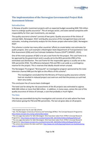
3. Page 3 of 8
The Project Cost Distribution
There is not much else to be inferred about the type of cost distribution from the graph. We
do not know whether those percentiles came from fitted distributions or from estimated
Pdf’s. This close relationship however leads us to believe that the individual projects cost
distributions are taken from the same family of distributions.
If this family of distributions is a two-parameter distribution, we can use the known P50 and
P85 percentiles to fit7 a number of distributions to the data.
This use of quantiles to estimate the parameters of an a priori distribution have been
described as "quantile maximum probability estimation" (Heathcote & al., 2004). This can be
done by fitting a number of different a priori distributions and then compare the sum log
likelihoods of the resulting best fits for each distribution, to find the “best” family of
distributions.
Using this we anticipate finding cost distributions with the following properties:
1. Nonsymmetrical, with a short left and a long right tail i.e. being positive skewed and
looking something like the distribution below (taken from a real life project):
2. The left tail we would expect to be short after the project has been run through the full
QA1 and QA2 process. After two such encompassing processes we would believe that
most, even if not all, possible avenues for cost reduction and grounds for miscalculations
have been researched and exhausted – leaving little room for cost reduction by chance.
3. The right tail we would expect to be long taking into account the possibility of adverse
price movements, implementation problems, adverse events etc. and thus the possibility
of higher costs. This is where the project risk lies and where budget overruns are born.
4. The middle part should be quite steep indicating low volatility around “most probable
cost”.
Estimating the Projects Cost Distribution
To simplify we will assume that the above relation between P50 and P85 holds, and that it
can be used to describe the resulting cost distribution from the projects QA2 risk assessment
work. We will hence use the P85/P50 ratio8 to study the cost distributions. This implies that
7
Most two-parameter families have sufficient flexibility to fit the P50 and P85 percentiles.
8
If costs is normally distributed: C ∼ N (m, s2
), then Z = C/m ∼ N (1, s2
/ m2). If costs is gamma distributed: C ∼ Γ
(a, λ) then Z = C/m ∼ Γ (1, λ).

4. Page 4 of 8
we are looking for a family of distributions that have the probability of (X<1) =0.5 and the
probability of (x<1.1) =0.85 and being positive skewed. This change of scale will not change the
shape of the density function, but simply scale the graph horizontally.
Fortunately the MD Anderson Cancer Centre has a program – Parameter Solver9 - that can
solve for the distribution parameters given the P50 and P85 percentiles (Cook, 2010). We
can then use this to find the distributions that can replicate the P50 and P85 percentiles.
We find that distributions from the Normal, Log Normal, Gamma, Inverse Gamma and
Weibull families will fit to the percentiles. All the distributions however are close to being
symmetric with the exception of the Weibull distribution that has a left tail. A left tail in a
budgeted cost distribution usually indicates over budgeting with the aim of looking good
after the project has been finished. We do not think that this would have passed the QA2
process – so we don’t think that it has been used.
We believe that it is most likely that the distributions used are of the Normal, Gamma or of
the Gamma derivative Erlang10 type, due to their convolution properties11. That is, sums of
independent identically distributed variables having one of these particular distributions
come from the same distribution family. This makes it possible to simplify risk models of the
cost only variety by just summing up the parameters12 of the cost elements to calculate the
parameters of the total cost distribution.
This have the benefit of giving the closed form for the total cost distribution compared to
Monte Carlo simulation where the closed form of the distribution, if it exists, only can be
found thru the exercise we have done here.
This property can as well be a trap, as the adding up of cost items quickly gives the
distribution of the sum symmetrical properties before it finally ends up as a Normal
distribution13.
The figures in the graph below give the shapes for the Gamma and Normal distribution with
the percentiles P50=1. and P85 = 1.1:
9
The software can be downloaded from:
https://biostatistics.mdanderson.org/SoftwareDownload/SingleSoftware.aspx?Software_Id=6
10
The Erlang distribution is a Gamma distribution with integer shape parameter.
11
For the Gamma and Erlang distribution the convolution property is restricted to distributions having the
same scale parameter.
12
For the Normal, Gamma and Erlang distributions this implies summing up the shape parameters of the
individual cost elements distribution:
If X and Y are normally distributed: X ∼ N (a, b2
) and Y∼ N (d, e2
) and X is independent of Y, then Z=X +
Y is N (a + d, b2
+ e2
), and if k is a strictly positive constant then Z=k*X is N (k*a, k2
* b2
).
If X and Y are gamma distributed: X ∼ Γ (a, λ) and Y∼ Γ (b, λ) and X is independent of Y, then X + Y is Γ
(a +b, λ), and if k is a strictly positive constant then c*X is Γ (k*a, λ).
13
The Central Limit Theorem gives the error in a normal approximation to the gamma distribution as n-1/2
as
the shape parameter n grows large. For large k the gamma distribution X ∼ Γ (k, θ) converges to a normal
distribution with mean µ = k*θ and variance s2
= k*θ2
. In practice it will approach a normal distribution with the
shape parameter > 10.

5. Page 5 of 8
The Normal distribution is symmetric and the Gamma distribution is also for all practical
purposes symmetric. We therefore can conclude that the distributions for total project cost
used in the 83 projects have been symmetric or close to symmetric distributions.
This result is quite baffling; it is difficult to understand why the project cost distributions
should be symmetric.
The only economic explanation have to be that the expected cost of the projects are
estimated with such precision that any positive or negative deviations are mere
flukes and chance outside foreseeability and thus not included in the risk
calculations.
But is this possible?
The two Large Military Projects
The two projects omitted from the regression above: new fighter planes and frigates have
values of the ratio P85/P50 as 1.19522 and 1.04543, compared to the regression estimate of
1.1001 for the 83 other projects. They are however not atypical, other among the 83
projects have both smaller (1.0310) and larger (1.3328) values for the P85/P50 ratio. Their
sheer size however with a P85 of respective 68 and 18 milliard NOK, gives them a too high
weight in a joint regression compared to the other projects.
Never the less, the same comments made above for the other 83 projects apply for these
two projects. A regression with the projects included would have given the relationship
between P85 and P50 as:
P85 = (+/- 0.0106+1.1751)* P50, with R= 0.9990.
And as shown in the graph below:

6. Page 6 of 8
This graph again depicts the surprisingly low variation in all the projects P85/P50 ratios:
The ratios have in point of fact a coefficient of variation of only 4.7% and a standard
deviation of 0.052 - for the all the 85 projects.
Conclusions
The Norwegian quality assurance scheme is obviously a large step in the direction of reduced
budget overruns in public projects14.
Even if the final risk calculation somewhat misses the probable project cost distribution will
the exercises described in the quality assurance scheme heighten both the risk awareness
and the uncertainty knowingness. All, contributing to the common goal – reduced budget
under- and overruns and reduced project cost.
It is nevertheless important that all elements in the quality assurance process catches the
project uncertainties15 in a correct way, describing each projects specific uncertainty and its
possible effects on project cost and implementation.
From what we have found: widespread use of symmetric cost distributions and possibly the
same type of distributions across the projects, we are a little doubtful about the methods
used for the risk calculations. The grounds for this are shown in the next two tables:
Cost estimates having a Gamma distribution
Project P85/P50 Shape Scale Mean Variance Skewnes Kurtosis
The 83 Projects 1.1000 114.8 0.0087 1.0029 0.0088 0.1867 0.0523
Minimum ratio 1.0310 1131.8 0.0009 1.0003 0.0009 0.0592 0.0053
Maximum ratio 1.3328 12.1 0.0851 1.0282 0.0875 0.5750 0.4959
Fighter Project 1.1952 32.1 0.0315 1.0105 0.0318 0.3530 0.1869
Frigates Project 1.0454 536.5 0.0019 1.0006 0.0019 0.0863 0.0112
The skewness16 given in the table above depends only on the shape parameter. The Gamma
distribution will approach a normal distribution when the parameter larger than ten. In this
case all projects’ cost distributions approach a normal distribution - that is a symmetric
distribution with zero skewness.
To us, this indicates that the projects’ cost distribution reflects more the engineer’s normal
calculation “errors” than the real risk for budget deviations due to implementation risk.
The kurtosis (excess kurtosis) indicates the form of the peak of the distribution. Normal
distributions have zero kurtosis (mesocurtic) while distributions with a high peak have a
positive kurtosis (leptokurtic).
14
See: Public Works Projects, http://www.strategy-at-risk.com/2009/09/03/public-works-projects/
15
See: Project Management under Uncertainty, http://www.strategy-at-risk.com/2014/08/01/project-
management-under-uncertainty/ .
16
The skewness is equal to two divided by the square root of the shape parameter.

7. Page 7 of 8
Cost estimates as having a Normal distribution
Project P85/P50 Mean Variance
The 83 Projects 1.1000 1.00 0.0093
Minimum ratio 1.0310 1.00 0.0099
Maximum ratio 1.3328 1.00 0.1031
Fighter Project 1.1952 1.00 0.0354
Frigates Project 1.0454 1.00 0.0019
It is stated in the QA2 that the uncertainty analysis shall have “special focus on … Event
uncertainties represented by a binary probability distribution” If this part had been
implemented we would have expected at least more flat-topped curves (platycurtic) with
negative kurtosis or better not only unimodal distributions. It is hard to see traces of this in
the material.
So, what can we so far deduct that the Norwegian government gets from the effort they
spend on risk assessment of their projects?
First, since the cost distributions most probably are symmetric or near symmetric,
expected cost will probably not differ significantly from the initial project cost
estimate (the engineering estimate) adjusted for reserves and risk margins. We
however need more data to substantiate this further.
Second, the P85 percentile could have been found by multiplying the P50 percentile
by 1.1. Finding the probability distribution for the projects’ cost has for the purpose
of establishing the P85 cost figures been unnecessary.
Third, the effect of event uncertainties seems to be missing.
Fourth, with such a variety of projects, it seems strange that the distributions for
total project cost ends up being so similar. There have to be differences in project risk
from building a road compared to a new Opera house.
Based on these findings it is pertinent to ask what went wrong in the implementation of
QA2. The idea is sound, but the result is somewhat disappointing.
The reason for this can be that the risk calculations are done just by assigning
probability distributions to the “aggregated and adjusted engineering “cost estimates
and not by developing a proper simulation model for the project, taking into
consideration uncertainties in all factors like quantities, prices, exchange rates,
project implementation etc.
We will come back in a later article to the question if the risk assessment never the less
reduces the budgets under- and overrun.
REFERENCES
Cook, John D. (2010), Determining distribution parameters from quantiles.
http://www.johndcook.com/quantiles_parameters.pdf

8. Page 8 of 8
Heathcote, A., Brown, S.& Cousineau, D. (2004). QMPE: estimating Lognormal, Wald, and
Weibull RT distributions with a parameter-dependent lower bound. Journal of Behavior
Research Methods, Instruments, and Computers (36), p. 277-290.
Washington State Department of Transportation (WSDOT), (2014), Project Risk Management Guide,
Nov 2014. http://www.wsdot.wa.gov/projects/projectmgmt/riskassessment