This pdf include basics of data Structure and algorithms

1. DATA STRUCTURE
Prof Vibhavari Pandit

2. 1. Arrays/List: (Weightage in % 15)
1. Introduction & Definition of an Array
2. Memory Allocation & Indexing
3. Operations on 1-D & 2D Arrays / Lists
4. Arrays and Their Applications
5. Sparse Matrices
6. String manipulation using arrays
7. Implementation of Polynomial using
Array
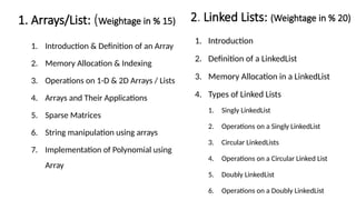
2. Linked Lists: (Weightage in % 20)
1. Introduction
2. Definition of a LinkedList
3. Memory Allocation in a LinkedList
4. Types of Linked Lists
1. Singly LinkedList
2. Operations on a Singly LinkedList
3. Circular LinkedLists
4. Operations on a Circular Linked List
5. Doubly LinkedList
6. Operations on a Doubly LinkedList

3. 3. Stacks and Queues (Weightage is % 20)
• IntroductionandDefinitionofa Stack
• ImplementationofaStack
• Implementation of Stacks Using Arrays
• Implementation of Stacks Using LinkedLists
• Applications of Stacks:
• Conversion of an expression(Infix,Prefix,Postfix)
• Evaluation of Expression
• String Reversal
• Introduction and Definition of a Queue
• Implementation of a Queue
• ImplementationofQueuesUsingArrays
• ImplementationofQueuesUsingLinkedLists
• ApplicationsofQueues
4. Tree & Graph (Weightage is % 25)
• TreeDefinition,representation
• BinarySearchTreeanditsoperations
• TreeTraversal
• Insertion
• Deletion
• Search
• AVLTreeanditsoperations
• Insertion
• Deletion
• Rotations
• DirectedandUndirectedGraph
• GraphRepresentations
• AdjacencyMatrix
• AdjacencyList
• GraphTraversals
• BFS
• DFS

4. Unit 5. Searching and Sorting
(Weightage is % 20)
• LinearSearchorSequential Search
• BinarySearch
• InterpolationSearch
• IntroductiontoSorting
• Merge Sort
• QuickSort
• BubbleSort
• Heap
• MinheapandMaxheap
• Hashing
• HashTable
• HashFunctions

5. What is Data Structure?
• Data structures are a specific way of organizing data in a specialized format on
a computer so that the information can be organized, processed, stored, and
retrieved quickly and effectively.
• They are a means of handling information, rendering the data for easy use.

6. Introduction of data structure
• The study of data structures helps to understand the basic concepts involved in
organizing and storing data as well as the relationship among the data sets. This in
turn helps to determine the way information is stored, retrieved and modified in a
computer’s memory.
• This in turn helps to determine the way information is stored, retrieved and
modified in a computer’s memory.

7. • Data structure is the structural representation of logical relationship between data
elements. This means that a data structure organizes data items based on the relationship
between the data elements.
Example:
A house can be identified by the house name, location, number of floors and so on.
These structured set of variables depend on each other to identify the exact house.
• Similarly, data structure is a structured set of variables that are linked to each other, which
forms the basic component of a system

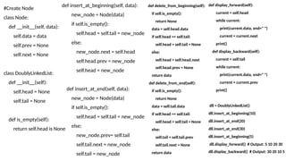
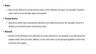
8. • Data:
• Data can be defined as an elementary value or the collection of values, for example, student's
name and its id are the data about the student.
• Group Items:
• Data items which have subordinate data items are called Group item, for example, name of a
student can have first name and the last name.
• Record:
• Record can be defined as the collection of various data items, for example, if we talk about the
student entity, then its name, address, course and marks can be grouped together to form the
record for the student.

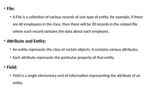
9. • File:
• A File is a collection of various records of one type of entity, for example, if there
are 60 employees in the class, then there will be 20 records in the related file
where each record contains the data about each employee.
• Attribute and Entity:
• An entity represents the class of certain objects. it contains various attributes.
• Each attribute represents the particular property of that entity.
• Field:
• Field is a single elementary unit of information representing the attribute of an
entity.

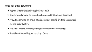
10. Need for Data Structure
• It gives different level of organization data.
• It tells how data can be stored and accessed in its elementary level.
• Provide operation on group of data, such as adding an item, looking up
highest priority item.
• Provide a means to manage huge amount of data efficiently.
• Provide fast searching and sorting of data.

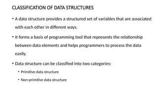
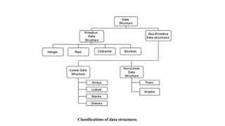
11. CLASSIFICATION OF DATA STRUCTURES
• A data structure provides a structured set of variables that are associated
with each other in different ways.
• It forms a basis of programming tool that represents the relationship
between data elements and helps programmers to process the data
easily.
• Data structure can be classified into two categories:
• Primitive data structure
• Non-primitive data structure

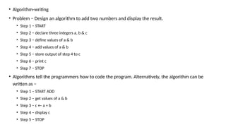
13. • Algorithm-writing
• Problem − Design an algorithm to add two numbers and display the result.
• Step 1 − START
• Step 2 − declare three integers a, b & c
• Step 3 − define values of a & b
• Step 4 − add values of a & b
• Step 5 − store output of step 4 to c
• Step 6 − print c
• Step 7 − STOP
• Algorithms tell the programmers how to code the program. Alternatively, the algorithm can be
written as −
• Step 1 − START ADD
• Step 2 − get values of a & b
• Step 3 − c ← a + b
• Step 4 − display c
• Step 5 − STOP

14. Classifications of data structures.

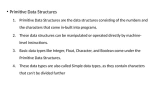
15. • Primitive Data Structures
1. Primitive Data Structures are the data structures consisting of the numbers and
the characters that come in-built into programs.
2. These data structures can be manipulated or operated directly by machine-
level instructions.
3. Basic data types like Integer, Float, Character, and Boolean come under the
Primitive Data Structures.
4. These data types are also called Simple data types, as they contain characters
that can't be divided further

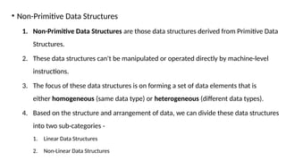
16. • Non-Primitive Data Structures
1. Non-Primitive Data Structures are those data structures derived from Primitive Data
Structures.
2. These data structures can't be manipulated or operated directly by machine-level
instructions.
3. The focus of these data structures is on forming a set of data elements that is
either homogeneous (same data type) or heterogeneous (different data types).
4. Based on the structure and arrangement of data, we can divide these data structures
into two sub-categories -
1. Linear Data Structures
2. Non-Linear Data Structures

17. • Linear Data Structures
• A data structure that preserves a linear connection among its data elements is
known as a Linear Data Structure. The arrangement of the data is done linearly,
where each element consists of the successors and predecessors except the first
and the last data element. However, it is not necessarily true in the case of
memory, as the arrangement may not be sequential.
• Based on memory allocation, the Linear Data Structures are further classified into
two types:
1. Static Data Structures:
2. Dynamic Data Structures:

18. 1. Static Data Structures: The data structures having a fixed size are known as Static Data
Structures. The memory for these data structures is allocated at the compiler time, and
their size cannot be changed by the user after being compiled; however, the data stored in
them can be altered.
The Array is the best example of the Static Data Structure as they have a fixed size, and its
data can be modified later.
2. Dynamic Data Structures: The data structures having a dynamic size are known as Dynamic
Data Structures. The memory of these data structures is allocated at the run time, and their
size varies during the run time of the code. Moreover, the user can change the size as well
as the data elements stored in these data structures at the run time of the code.
Linked Lists, Stacks, and Queues are common examples of dynamic data
structures

19. • Types of Linear Data Structures
The following is the list of Linear Data Structures that we generally use:
1. Arrays
2. Linked Lists
3. Stacks
4. Queues

20. • Non-Linear Data Structures
• Non-Linear Data Structures are data structures where the data elements are not
arranged in sequential order. Here, the insertion and removal of data are not
feasible in a linear manner. There exists a hierarchical relationship between the
individual data items.
• Types of Non-Linear Data Structures
1. Trees
2. Graphs

21. • Basic Operations of Data Structures
1. Traversal
2. Search
3. Insertion
4. Deletion
5. Sorting
6. Merge
7. Create
8. Selection
9. Update

22. Array
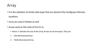
• It is the collection of similar data types that are stored in the Contiguous Memory
Locations.
• Array are used in Python as well.
• Arrays work on the scale of 0 to (n-1),
• where ‘n’ denotes the size of the array. Arrays are of two types. They are:
1. One-dimensional Array
2. Multi-dimensional Array

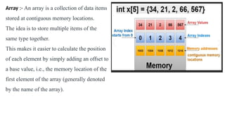
23. Array :- An array is a collection of data items
stored at contiguous memory locations.
The idea is to store multiple items of the
same type together.
This makes it easier to calculate the position
of each element by simply adding an offset to
a base value, i.e., the memory location of the
first element of the array (generally denoted
by the name of the array).

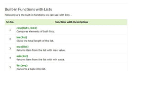
24. Python Array
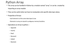
• The array can be handled in Python by a module named “array” or can be created by
importing an array module
• They can be useful when we have to manipulate only specific data type values.
• Properties of Arrays
- Each element is of the same data types & size
- Elements in array are stored in contiguous memory locations.
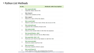
- Operations on Array in python :-
- Append()
- Insert()
- Pop()
- Remove()
- Index()
- Reverse()

25. • Syntax:-
• array(data_type, value list)
example
1) import array as arr
array1=arr.array('i' , [1,2,3])
print ("the new created array is:")
for i in range(0,3):
print (array1[ i ])
Output= the new created array is:
1
2
3
2)import array as arr
array1 = arr.array('i', [10,20,30,40,50])
print (array1[0])
print (array1[2])
Output = 10
30

26. 1) Append () :
To add a new element to an array, use the append() method.
It accepts a single item as an argument and append it at the end of given array.
import array as arr
array1=arr.array( ‘i’ , [1, 2 ,3] )
print (“The element of array is:”)
for i in range(0,3):
print (array1[ i ]) [1, 2, 3]
array1.append(4)
print (“Appended array is :”)
for i in range(len(array1))
print(array1[i]) [1, 2, 3,4]

27. 2) insert (i , x ) where i is the position and x is value
Example1:
import array as arr
array1=arr.array( ‘i’ , [1, 2 ,3,4] )
array1.insert(2,5)
Print (“Array after inserting 5 at 2nd
position is:”, end= “ “)
for i in range( len ( array1 ) )
print (array1[ i ])
3) Remove Items from Specific Indices
pop(i) where i is the position
import array as arr
array1=arr.array( ‘i’ , [1, 2 ,3, 4, 5] )
Print (“New Array is : ” , end = “ “)
for i in range( len ( array1 ) )
print (array1[ i ], end = “ “)
print (array1.pop(2)) pop element 3
for i in range( len ( array1 ) )
print (array1[ i ]) [1, 2, ,4, 5]
Example 2:
import array as arr
array1 =arr. array('i', [10,20,30,40,50])
array1.insert(1,60)
for x in array1:
print(x)

28. 4) array remove (a) where a is value
To remove the first occurrence of a given value from the array, use remove() method. This method accepts an element and removes it if the
element is available in the array.
import array as arr
array1=arr.array( ‘i’ , [1, 2 ,3, 1, 4, 5 ] )
array1.remove(1) output is[ 2, 3, 1, 4, 5 ]
for x in array1:
print(x)
5) Search Operation : Search a data element in an array & return index.
index(a) where a is value
import array as arr
array1=arr.array( ‘i’ , [1, 2 ,3, 1, 2, 5 ] )
print(array1.index(2)) output is 1
6) reverse()
import array as arr
array1=arr.array( 'i' , [1, 2, 3, 1, 4, 5 ] )
array1.reverse()
for i in range( len ( array1 ) ):
print (array1[ i ] ) [ 5, 4, 1, 3, 2, 1 ]
array1 =arr. array('i', [10,20,30,40,50])
array1.remove(40)
for x in array1:
print(x)

29. 7) Array Typecode function
( ‘i’ , [1, 2, 3, 4] )
print (array1.typecode)
Returns type of array elements output is i
8) Itemsize where a is value
( ‘i’ , [1, 2, 3, 4] )
array1=arr.array( ‘i’ , [1, 2 ,3, 1, 2, 5 ] ) return the size of elements in currency all are integer
print (array1.itemsize) output is 4
9) buffer_info()
( ‘i’ , [1, 2, 3, 4] )
print (array1.buffer_info() return (1404912603686813, 4)
10) count(4) where 4 is value
count the no. of occurrences of argument mentioned in array.

30. 11) extend()
array1=arr.array( ‘i’ , [1, 2 ,3 ] )
array2=arr.array( ‘i’ , [4,5,6 ] )
array1.extend(array2)
for i in range(len(array1)):
print(array1)
12) fromlist(add the list at the end of array)
array1=arr.array( ‘i’ , [1, 2 ,3] )
li=[1, 2, 3]
array1=fromlist(li)
for i in range( len ( array1 ) )
print (array1) [ 1, 2, 3, 1, 2, 3]
13) tolist(transform any array to list)
array1=arr.array( ‘i’ , [1, 2 ,3,4] )
li=aaray1.tolist()
Output is [ 1, 2, 3, 4 ]

31. • Update Operation
import array as arr
array1=arr.array('i', [10,20,30,40,50])
array1[2] = 80
for x in array1:
print(x)
Output : 10
20
80
40
50

32. • Sorting of array :
• import array as arr a = arr.array('i', [10,5,15,4,6,20,9])
• for i in range(0, len(a)):
• for j in range(i+1, len(a)):
• if(a[i] > a[j]):
• temp = a[i];
• a[i] = a[j];
• a[j] = temp;
• print (a)

33. • Sort Arrays Using sort() Method of List
• import array as arr
• # creating array
• orgnlArray = arr.array('i', [10,5,15,4,6,20,9])
• print("Original array:", orgnlArray)
• # converting to list
• sortedList = orgnlArray.tolist()
• # sorting the list
• sortedList.sort()
• # creating array from sorted list
• sortedArray = arr.array('i', sortedList)
• print("Array after sorting:",sortedArray)

34. List
• List is one of the built-in data types in Python. A Python list is a sequence of comma separated items, enclosed in square
brackets [ ]. The items in a Python list need not be of the same data type.
• List is an ordered collection of items. Each item in a list has a unique position index, starting from 0.
• List=[] -> creates blank list
• List = [10, 20, 14]
print("nList of numbers: ") output = List of numbers:
print(List) [10, 20, 14]
• list1 = ["Rohan", "Physics", 21, 69.75]
• list2 = [1, 2, 3, 4, 5]
• list3 = ["a", "b", "c", "d"]
• list4 = [25.50, True, -55, 1+2j]
• list5 = [1,2,'raj','komal',78]
print(list4[3]) output = komal

35. • list1 = ['physics', 'chemistry', 1997, 2000];
• list2 = [1, 2, 3, 4, 5, 6, 7 ];
• print ("list1[0]: ", list1[0])
• print ("list2[1:5]: ", list2[1:5])
• Output :
• list1[0]: physics
• list2[1:5]: [2, 3, 4, 5]

36. Multidimensional List
List=[['Ram','Sham'],['Sita','Gita']]
print (List[0][1]) output = Sham
print(List[1][0]) output = Sita

37. • Updating Lists :
• list = ['physics', 'chemistry', 1997, 2000];
• print ("Value available at index 2 : ")
• print (list[2])
• list[2] = 2001;
• print ("New value available at index 2 : ")
• print (list[2])
Output
Value available at index 2 :
1997
New value available at index 2 :
2001

38. • Delete List Elements:-
list1 = ['physics', 'chemistry', 1997, 2000];
print (list1)
del list1[2];
print ("After deleting value at index 2 : ")
print (list1)
Output
['physics', 'chemistry', 1997, 2000]
After deleting value at index 2 :
['physics', 'chemistry', 2000]

39. Append :-
• List=[]
Print(List)
• List.append(10)
List.append(20)
List.append(30)
print(List) output=[10,20,30]
Adding elements to the list using iterator
• List=[10,20,30]
for i in range(1,4)
List.append(i)
print(List) output=[10,20,30,1,2,3]
Adding list to the list
• List=[1,2,3]
List2=["for","is"]
List.append(List2)
print(List) output= [1, 2, 3, ['for', 'is']]

40. • Insert Operation
Syntax - insert(index,value)
• List=[1,2,3]
• List2=["for","is"]
• List.append(List2)
• print(List)
• List.insert(3,13)
• print(List)
Output = [1, 2, 3, ['for', 'is']]
[1, 2, 3, 13, ['for', 'is']]

41. Extend Function (Adding multiple elements at the end)
• List=[1,2,3]
• List.extend([7,'ram','sham'])
• print(List) Output = [1, 2, 3, 7, 'ram', 'sham']
Reversed Function
• Mylist=[4,5,6]
• Rev_list=list(reversed(Mylist))
• print(Rev_list) Output = [6, 5, 4]
Remove Function
• Mylist=[4,5,6,7,8]
• Mylist.remove(4)
• print(Mylist) Output = [5, 6, 7, 8]

42. • Python List Methods

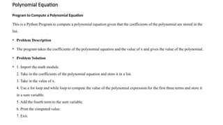
44. Polynomial Equation
Program to Compute a Polynomial Equation
This is a Python Program to compute a polynomial equation given that the coefficients of the polynomial are stored in the
list.
• Problem Description
• The program takes the coefficients of the polynomial equation and the value of x and gives the value of the polynomial.
• Problem Solution
• 1. Import the math module.
2. Take in the coefficients of the polynomial equation and store it in a list.
3. Take in the value of x.
4. Use a for loop and while loop to compute the value of the polynomial expression for the first three terms and store it
in a sum variable.
5. Add the fourth term to the sum variable.
6. Print the computed value.
7. Exit.

45. Program/Source Code
import math
print("Enter the coefficients of the form ax^3 + bx^2 + cx + d")
lst=[]
for i in range(0,4):
a=int(input("Enter coefficient:"))
lst.append(a)
x=int(input("Enter the value of x:"))
sum1=0
j=3
for i in range(0,3):
while(j>0):
sum1=sum1+(lst[i]*math.pow(x,j))
break
j=j-1
sum1=sum1+lst[3]
print("The value of the polynomial is:",sum1)
Program Explanation
1. The math module is imported.
2. User must enter the coefficients of the polynomial which is
stored in a list.
3. User must also enter the value of x.
4. The value of i ranges from 0 to 2 using the for loop which is
used to access the coefficients in the list.
5. The value of j ranges from 3 to 1, which is used to determine
the power for the value of x.
6. The value of the first three terms is computed this way.
7. The last term is added to the final sum.
8. The final computed value is printed.

46. • def eval(poly, n, x):
• result = poly[0]
• for i in range(1, n):
• result = result*x + poly[i]
• return result
• poly = [2, 0, 3, 1]
• x = 2
• n = len(poly)
• print("Value of polynomial is " , eval(poly, n, x))

47. • Polynomial Addiontion
• def add_polynomials(poly1, poly2):
•
• max_len = max(len(poly1), len(poly2))
•
•
• result = [0] * max_len
•
• for i in range(len(poly1)):
• result[i] += poly1[i]
• for i in range(len(poly2)):
• result[i] += poly2[i]
•
• return result
• poly1 = [3,0,0, 2, 5] # Represents 3 + 2x + 5x^2
• poly2 = [5, 1, 2, 4] # Represents 5 + x + 2x^2 + 4x^3
• result = add_polynomials(poly1, poly2)
• print("Resultant polynomial coefficients:", result)

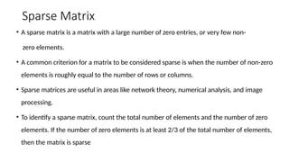
48. Sparse Matrix
• A sparse matrix is a matrix with a large number of zero entries, or very few non-
zero elements.
• A common criterion for a matrix to be considered sparse is when the number of non-zero
elements is roughly equal to the number of rows or columns.
• Sparse matrices are useful in areas like network theory, numerical analysis, and image
processing.
• To identify a sparse matrix, count the total number of elements and the number of zero
elements. If the number of zero elements is at least 2/3 of the total number of elements,
then the matrix is sparse

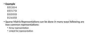
49. • Example
0 0 3 0 4
0 0 5 7 0
0 0 0 0 0
0 2 6 0 0
• Sparse Matrix Representations can be done in many ways following are
two common representations:
• Array representation
• Linked list representation

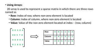
50. • Using Arrays:
2D array is used to represent a sparse matrix in which there are three rows
named as
• Row: Index of row, where non-zero element is located
• Column: Index of column, where non-zero element is located
• Value: Value of the non zero element located at index – (row, column)

51. • Advantage over simple matrix
1. Storage :- there are lesser non-zero elements than zeros and thus
lesser memory can be used to store only those elements.
2. Computing time: Computing time can be saved by logically designing a
data structure traversing only non-zero elements..

52. • dense_matrix = [
• [0, 0, 3, 0],
• [4, 0, 0, 5],
• [0, 6, 0, 0],
• [0, 0, 0, 0]
• ]
• # Initialize an empty list to hold the sparse matrix representation
• sparse_matrix = []
• print(len(dense_matrix))
• # Iterate through the dense matrix
• for i in range(len(dense_matrix)):
• for j in range(len(dense_matrix[i])):
• # If the element is non-zero, store its row index, column index, and value
• if dense_matrix[i][j] != 0:
• sparse_matrix.append((i, j, dense_matrix[i][j]))
• # Output the sparse matrix
• print("Sparse Matrix Representation (row, column, value):")
• for item in sparse_matrix:
• print(item)
Output :
4
Sparse Matrix Representation (row, column, value):
(0, 2, 3)
(1, 0, 4)
(1, 3, 5)
(2, 1, 6)

53. Link List
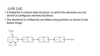
• A linked list is a linear data structure, in which the elements are not
stored at contiguous memory locations.
• The elements in a linked list are linked using pointers as shown in the
below image:

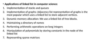
54. • Applications of linked list in computer science:
1. Implementation of stacks and queues
2. Implementation of graphs: Adjacency list representation of graphs is the
most popular which uses a linked list to store adjacent vertices.
3. Dynamic memory allocation: We use a linked list of free blocks.
4. Maintaining a directory of names
5. Performing arithmetic operations on long integers
6. Manipulation of polynomials by storing constants in the node of the
linked list
7. Representing sparse matrices

55. • Applications of linked list in the real world:
1. Image viewer – Previous and next images are linked and can be accessed
by the next and previous buttons.
2. Previous and next page in a web browser – We can access the previous
and next URL searched in a web browser by pressing the back and next
buttons since they are linked as a linked list.
3. Music Player – Songs in the music player are linked to the previous and
next songs. So you can play songs either from starting or ending of the list.
4. GPS navigation systems- Linked lists can be used to store and manage a list
of locations and routes, allowing users to easily navigate to their desired
destination.
5. Robotics- Linked lists can be used to implement control systems for
robots, allowing them to navigate and interact with their environment.

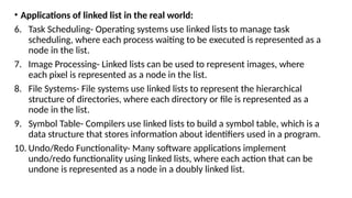
56. • Applications of linked list in the real world:
6. Task Scheduling- Operating systems use linked lists to manage task
scheduling, where each process waiting to be executed is represented as a
node in the list.
7. Image Processing- Linked lists can be used to represent images, where
each pixel is represented as a node in the list.
8. File Systems- File systems use linked lists to represent the hierarchical
structure of directories, where each directory or file is represented as a
node in the list.
9. Symbol Table- Compilers use linked lists to build a symbol table, which is a
data structure that stores information about identifiers used in a program.
10. Undo/Redo Functionality- Many software applications implement
undo/redo functionality using linked lists, where each action that can be
undone is represented as a node in a doubly linked list.

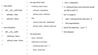
57. • class Node:
• def __init__(self, data):
• self.data = data
• self.next = None
•
• class LinkedList:
• def __init__(self):
• self.head = None
• self.last_node = None
•
• def append(self, data):
• if self.last_node is None:
• self.head = Node(data)
• self.last_node = self.head
• else:
• self.last_node.next = Node(data)
• self.last_node = self.last_node.next
•
• def display(self):
• temp = self.head
• while temp is not None:
• print(temp.data, end = ' ')
• temp = temp.next
•
• list1 = LinkedList()
• n = int(input('How many elements would
you like to add? '))
• for i in range(n):
• data = int(input('Enter data item: '))
• list1.append(data)
• print('The linked list: ', end = '')
• list1.display()

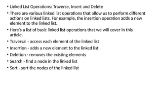
58. • Linked List Operations: Traverse, Insert and Delete
• There are various linked list operations that allow us to perform different
actions on linked lists. For example, the insertion operation adds a new
element to the linked list.
• Here's a list of basic linked list operations that we will cover in this
article.
• Traversal - access each element of the linked list
• Insertion - adds a new element to the linked list
• Deletion - removes the existing elements
• Search - find a node in the linked list
• Sort - sort the nodes of the linked list

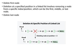
59. • Delete first node
• Deletion at a specified position in a linked list involves removing a node
from a specific index/position, which can be the first, middle, or last
node.
• Delete last node

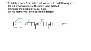
60. • To delete a node from linked list, we need to do following steps.
1) Find previous node of the node to be deleted.
2) Change the next of previous node.
3) Free memory for the node to be deleted.

61. Insertion in singly linked list at beginning
Algorithm
Step 1: IF PTR = NULL
Write OVERFLOW
Go to Step 7
[END OF IF]
Step 2: SET NEW_NODE = PTR
Step 3: SET PTR = PTR → NEXT
Step 4: SET NEW_NODE → DATA = VAL
Step 5: SET NEW_NODE → NEXT = HEAD
Step 6: SET HEAD = NEW_NODE
Step 7: EXIT
Deletion algorithm
1. If the head node has the given key,
make the head node points to the second node and free its memory.
2. Otherwise,
From the current node, check whether the next node has the given key
if yes, make the current->next = current->next->next and free the memory.
else, update the current node to the next and do the above process (from step 2) till the last node.

62. • class Node:
• def __init__(self, data):
• self.data = data
• self.next = None
•
• class LinkedList:
• def __init__(self):
• self.head = None
• self.last_node = None
•
• def append(self, data):
• if self.last_node is None:
• self.head = Node(data)
• self.last_node = self.head
• else:
• self.last_node.next = Node(data)
• self.last_node = self.last_node.next
• def display(self):
• temp = self.head
• while temp is not None:
• print(temp.data, end = ' ')
• temp = temp.next
•
• a_llist = LinkedList()
• n = int(input('How many elements would you like to add?
'))
• for i in range(n):
• data = int(input('Enter data item: '))
• a_llist.append(data)
• print('The linked list: ', end = '')
• a_llist.display()
• a_llist.remove_first_node()
• print('nThe linked list: ', end = '')
• a_llist.display()
• a_llist.remove_last_node()
• print('nThe linked list: ', end = '')
• a_llist.display()
• a_llist.insert(79,2)
• print('The linked list: ', end = '')
• a_llist.display()
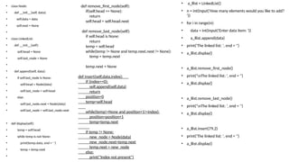
def remove_first_node(self):
if(self.head == None):
return
self.head = self.head.next
def remove_last_node(self):
if self.head is None:
return
temp = self.head
while(temp != None and temp.next.next != None):
temp = temp.next
temp.next = None
def insert(self,data,index):
if (index==0):
self.append(self,data)
return
position=0
temp=self.head
while(temp!=None and position+1!=index):
position=position+1
temp=temp.next
if temp != None:
new_node = Node(data)
new_node.next=temp.next
temp.next = new_node
else:
print("Index not present")

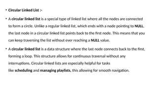
63. • Circular Linked List :-
• A circular linked list is a special type of linked list where all the nodes are connected
to form a circle. Unlike a regular linked list, which ends with a node pointing to NULL,
the last node in a circular linked list points back to the first node. This means that you
can keep traversing the list without ever reaching a NULL value.
• A circular linked list is a data structure where the last node connects back to the first,
forming a loop. This structure allows for continuous traversal without any
interruptions. Circular linked lists are especially helpful for tasks
like scheduling and managing playlists, this allowing for smooth navigation.

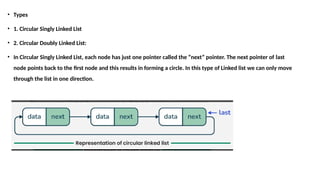
64. • Types
• 1. Circular Singly Linked List
• 2. Circular Doubly Linked List:
• In Circular Singly Linked List, each node has just one pointer called the “next” pointer. The next pointer of last
node points back to the first node and this results in forming a circle. In this type of Linked list we can only move
through the list in one direction.

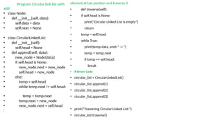
65. Program Circular link list with
add
• class Node:
• def __init__(self, data):
• self.data = data
• self.next = None
• class CircularLinkedList:
• def __init__(self):
• self.head = None
• def append(self, data):
• new_node = Node(data)
• if self.head is None:
• new_node.next = new_node
• self.head = new_node
• else:
• temp = self.head
• while temp.next != self.head:
• temp = temp.next
• temp.next = new_node
• new_node.next = self.head
•
•
element at last position and traverse it
• def traverse(self):
• if self.head is None:
• print("Circular Linked List is empty")
• return
• temp = self.head
• while True:
• print(temp.data, end=" -> ")
• temp = temp.next
• if temp == self.head:
• break
• # Driver Code
• circular_list = CircularLinkedList()
• circular_list.append(1)
• circular_list.append(2)
• circular_list.append(3)
• print("Traversing Circular Linked List:")
• circular_list.traverse()

66. • Program Circular link list
• class Node:
• def __init__(self, data):
• self.data = data
• self.next = None
• class CircularLinkedList:
• def __init__(self):
• # Initialize an empty circular linked
list with head pointer pointing to None
• self.head = None
#Append the Node
def append(self, data):
# Append a new node with data to the end of the circular linked list
new_node = Node(data)
if self.head is None:
# If the list is empty, make the new node point to itself
new_node.next = new_node
self.head = new_node
else:
temp = self.head
while temp.next != self.head:
# Traverse the list until the last node
temp = temp.next
# Make the last node point to the new node
temp.next = new_node
# Make the new node point back to the head
new_node.next = self.head
# Traverse the List
def traverse(self):
# Traverse and display the elements of the circular linked list
if self.head is None:
print("Circular Linked List is empty")
return
temp = self.head
while True:
print(temp.data, end=" -> ")
temp = temp.next
if temp == self.head:
# Break the loop when we reach the head again
break
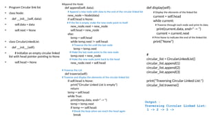
def display(self):
# Display the elements of the linked list
current = self.head
while current:
# Traverse through each node and print its data
print(current.data, end=" -> ")
current = current.next
# Print None to indicate the end of the linked list
print("None")
#
circular_list = CircularLinkedList()
circular_list.append(1)
circular_list.append(2)
circular_list.append(3)
print("Traversing Circular Linked List:")
circular_list.traverse()
Output :
Traversing Circular Linked List:
1 -> 2 -> 3 ->

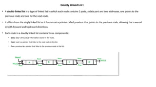
67. Doubly Linked List :
• A doubly linked list is a type of linked list in which each node contains 3 parts, a data part and two addresses, one points to the
previous node and one for the next node.
• It differs from the singly linked list as it has an extra pointer called previous that points to the previous node, allowing the traversal
in both forward and backward directions.
• Each node in a doubly linked list contains three components:
• Data: data is the actual information stored in the node.
• Next: next is a pointer that links to the next node in the list.
• Prev: previous is a pointer that links to the previous node in the list.

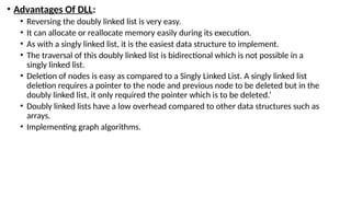
68. • Advantages Of DLL:
• Reversing the doubly linked list is very easy.
• It can allocate or reallocate memory easily during its execution.
• As with a singly linked list, it is the easiest data structure to implement.
• The traversal of this doubly linked list is bidirectional which is not possible in a
singly linked list.
• Deletion of nodes is easy as compared to a Singly Linked List. A singly linked list
deletion requires a pointer to the node and previous node to be deleted but in the
doubly linked list, it only required the pointer which is to be deleted.’
• Doubly linked lists have a low overhead compared to other data structures such as
arrays.
• Implementing graph algorithms.

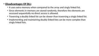
69. • Disadvantages Of DLL:
• It uses extra memory when compared to the array and singly linked list.
• Since elements in memory are stored randomly, therefore the elements are
accessed sequentially no direct access is allowed.
• Traversing a doubly linked list can be slower than traversing a singly linked list.
• Implementing and maintaining doubly linked lists can be more complex than
singly linked lists.

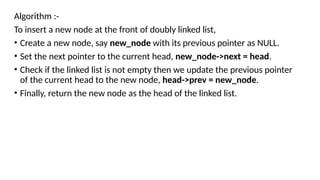
70. Algorithm :-
To insert a new node at the front of doubly linked list,
• Create a new node, say new_node with its previous pointer as NULL.
• Set the next pointer to the current head, new_node->next = head.
• Check if the linked list is not empty then we update the previous pointer
of the current head to the new node, head->prev = new_node.
• Finally, return the new node as the head of the linked list.

71. #Create Node
class Node:
def __init__(self, data):
self.data = data
self.prev = None
self.next = None
class DoublyLinkedList:
def __init__(self):
self.head = None
self.tail = None
def is_empty(self):
return self.head is None
def insert_at_beginning(self, data):
new_node = Node(data)
if self.is_empty():
self.head = self.tail = new_node
else:
new_node.next = self.head
self.head.prev = new_node
self.head = new_node
def insert_at_end(self, data):
new_node = Node(data)
if self.is_empty():
self.head = self.tail = new_node
else:
new_node.prev= self.tail
self.tail.next = new_node
self.tail = new_node
def delete_from_beginning(self):
if self.is_empty():
return None
data = self.head.data
if self.head == self.tail:
self.head = self.tail = None
else:
self.head = self.head.next
self.head.prev = None
return data
def delete_from_end(self):
if self.is_empty():
return None
data = self.tail.data
if self.head == self.tail:
self.head = self.tail = None
else:
self.tail = self.tail.prev
self.tail.next = None
return data
def display_forward(self):
current = self.head
while current:
print(current.data, end=" ")
current = current.next
print()
def display_backward(self):
current = self.tail
while current:
print(current.data, end=" ")
current = current.prev
print()
dll = DoublyLinkedList()
dll.insert_at_beginning(10)
dll.insert_at_end(20)
dll.insert_at_end(30)
dll.insert_at_beginning(5)
dll.display_forward() # Output: 5 10 20 30
dll.display_backward() # Output: 30 20 10 5