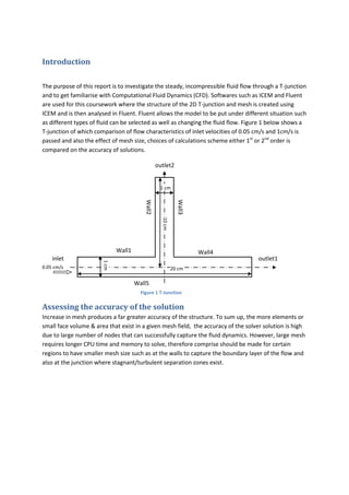
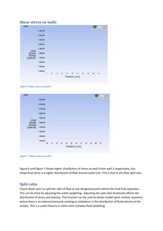
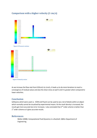
Introduction

The purpose of this report is to investigate the steady, incompressible fluid flow through a T-junction
and to get familiarise with Computational Fluid Dynamics (CFD). Softwares such as ICEM and Fluent
are used for this coursework where the structure of the 2D T-junction and mesh is created using
ICEM and is then analysed in Fluent. Fluent allows the model to be put under different situation such
as different types of fluid can be selected as well as changing the fluid flow. Figure 1 below shows a
T-junction of which comparison of flow characteristics of inlet velocities of 0.05 cm/s and 1cm/s is
passed and also the effect of mesh size, choices of calculations scheme either 1st or 2nd order is
compared on the accuracy of solutions.

                                                  outlet2


                                                   1 cm
                                          Wall2


                                                              Wall3
                                                    10 cm


                              Wall1                                   Wall4
    inlet                                                                           outlet1
                       1 cm


0.05 cm/s                                                   20 cm

                                      Wall5
                                        Figure 1 T-Junction

Assessing the accuracy of the solution
Increase in mesh produces a far greater accuracy of the structure. To sum up, the more elements or
small face volume & area that exist in a given mesh field, the accuracy of the solver solution is high
due to large number of nodes that can successfully capture the fluid dynamics. However, large mesh
requires longer CPU time and memory to solve, therefore comprise should be made for certain
regions to have smaller mesh size such as at the walls to capture the boundary layer of the flow and
also at the junction where stagnant/turbulent separation zones exist.
Increasing/Reducing the mesh density in ICEM
Increasing mesh density reduces cell size, this effectively increases accuracy however due to
truncation error this is not always the case. The reduction in cell size allows convergence to be
reached earlier but this requires a lot of memory and also requires higher processing abilities. For a
2D t-junction the shapes components are not complex so simple meshes will be sufficient to show
flow and velocity gradients.


                                    Figure 2 mesh size 50
Figure 3 mesh size 30


Influence of 2nd and 1st order
The choice of calculation scheme (1st or 2nd order upwind) also affects the accuracy of the results. As
discussed above the flow through the 2D structure is largely viscous flow which involves second
order differentials compared to inviscid flows where only first order differentials are involved. Using
higher order scheme also reduces the truncation errors, but requires increased CPU time and
memory. Therefore the second order scheme is more accurate than the first order results. I
personally used 1st order scheme as a lot a precision isn’t required in this report.


Unstructured and structured grid
Structured grid has a more uniform mesh for simpler shapes which have no irregularities for this
specific problem. Where a t-junction is concerned a structured grid gives better results due to its
rectangular components in complex shapes. Using an unstructured grid would be a better option as
the mesh will be more flexible and cells will be appropriately placed.
Flow visualization


Figure 4 pressure contour for mesh size 30


 Figure 5 velocity vector plot for mesh size 30

 Static pressure contour shows high pressure at the inlet where velocity profile is developing,
 pressure reduces as the flow reaches the outlet. Velocity vector field shows that the no slip
 boundary condition has been met and velocity reduce before splitting up. It also shows velocity to be
 maximum on the centre at any point.
Shear stress on walls


Figure 6 Shear stress on wall 3


Figure 7 Shear stress on wall 4


Figure 6 and Figure 7 shows higher distribution of stress on wall 4 than wall 3 respectively, this
shows that there is a higher distribution of flow around outlet one. This is due to the flow split ratio.


Split ratio
Fluent allow users to split the ratio of flow at any designated point where the fluid flow separates.
This can be done by adjusting the outlet weighting. Adjusting the split ratio drastically affects the
distribution of stress and velocity. This function can be used to better model some realistic scenarios
where there is an external pressure creating an imbalance in the distribution of fluid velocity at the
outlets. This is a useful feature in some more complex fluid modelling.
Comparison with a higher velocity (1 cm/s)


  Figure 8 Pressure contour


 Figure 9 Velocity vector


As we increase the flow rate from 0.05cm/s to 1cm/s, it leads us to do more iterations to reach a
convergence of residual values and also the shear stress at wall 3 and 4 is greater when compared to
lower velocities.


Conclusion
Softwares which were used i.e. ICEM and Fluent can be used to see a lot of details within an object
which normally cannot be visualised by experimental means. As the mesh density is increased, the
results get more accurate but error increases. I also concluded that 2nd order scheme is better than
1st order scheme as it gives accurate results.


References
         Müller (2008). Computational Fluid Dynamics in a Nutshell. QMUL Department of
         Engineering.

T junction report

  • 1.
    Introduction The purpose ofthis report is to investigate the steady, incompressible fluid flow through a T-junction and to get familiarise with Computational Fluid Dynamics (CFD). Softwares such as ICEM and Fluent are used for this coursework where the structure of the 2D T-junction and mesh is created using ICEM and is then analysed in Fluent. Fluent allows the model to be put under different situation such as different types of fluid can be selected as well as changing the fluid flow. Figure 1 below shows a T-junction of which comparison of flow characteristics of inlet velocities of 0.05 cm/s and 1cm/s is passed and also the effect of mesh size, choices of calculations scheme either 1st or 2nd order is compared on the accuracy of solutions. outlet2 1 cm Wall2 Wall3 10 cm Wall1 Wall4 inlet outlet1 1 cm 0.05 cm/s 20 cm Wall5 Figure 1 T-Junction Assessing the accuracy of the solution Increase in mesh produces a far greater accuracy of the structure. To sum up, the more elements or small face volume & area that exist in a given mesh field, the accuracy of the solver solution is high due to large number of nodes that can successfully capture the fluid dynamics. However, large mesh requires longer CPU time and memory to solve, therefore comprise should be made for certain regions to have smaller mesh size such as at the walls to capture the boundary layer of the flow and also at the junction where stagnant/turbulent separation zones exist.
  • 2.
    Increasing/Reducing the meshdensity in ICEM Increasing mesh density reduces cell size, this effectively increases accuracy however due to truncation error this is not always the case. The reduction in cell size allows convergence to be reached earlier but this requires a lot of memory and also requires higher processing abilities. For a 2D t-junction the shapes components are not complex so simple meshes will be sufficient to show flow and velocity gradients. Figure 2 mesh size 50 Figure 3 mesh size 30 Influence of 2nd and 1st order The choice of calculation scheme (1st or 2nd order upwind) also affects the accuracy of the results. As discussed above the flow through the 2D structure is largely viscous flow which involves second order differentials compared to inviscid flows where only first order differentials are involved. Using higher order scheme also reduces the truncation errors, but requires increased CPU time and memory. Therefore the second order scheme is more accurate than the first order results. I personally used 1st order scheme as a lot a precision isn’t required in this report. Unstructured and structured grid Structured grid has a more uniform mesh for simpler shapes which have no irregularities for this specific problem. Where a t-junction is concerned a structured grid gives better results due to its rectangular components in complex shapes. Using an unstructured grid would be a better option as the mesh will be more flexible and cells will be appropriately placed.
  • 3.
    Flow visualization Figure 4pressure contour for mesh size 30 Figure 5 velocity vector plot for mesh size 30 Static pressure contour shows high pressure at the inlet where velocity profile is developing, pressure reduces as the flow reaches the outlet. Velocity vector field shows that the no slip boundary condition has been met and velocity reduce before splitting up. It also shows velocity to be maximum on the centre at any point.
  • 4.
    Shear stress onwalls Figure 6 Shear stress on wall 3 Figure 7 Shear stress on wall 4 Figure 6 and Figure 7 shows higher distribution of stress on wall 4 than wall 3 respectively, this shows that there is a higher distribution of flow around outlet one. This is due to the flow split ratio. Split ratio Fluent allow users to split the ratio of flow at any designated point where the fluid flow separates. This can be done by adjusting the outlet weighting. Adjusting the split ratio drastically affects the distribution of stress and velocity. This function can be used to better model some realistic scenarios where there is an external pressure creating an imbalance in the distribution of fluid velocity at the outlets. This is a useful feature in some more complex fluid modelling.
  • 5.
    Comparison with ahigher velocity (1 cm/s) Figure 8 Pressure contour Figure 9 Velocity vector As we increase the flow rate from 0.05cm/s to 1cm/s, it leads us to do more iterations to reach a convergence of residual values and also the shear stress at wall 3 and 4 is greater when compared to lower velocities. Conclusion Softwares which were used i.e. ICEM and Fluent can be used to see a lot of details within an object which normally cannot be visualised by experimental means. As the mesh density is increased, the results get more accurate but error increases. I also concluded that 2nd order scheme is better than 1st order scheme as it gives accurate results. References Müller (2008). Computational Fluid Dynamics in a Nutshell. QMUL Department of Engineering.