Download as PDF, PPTX

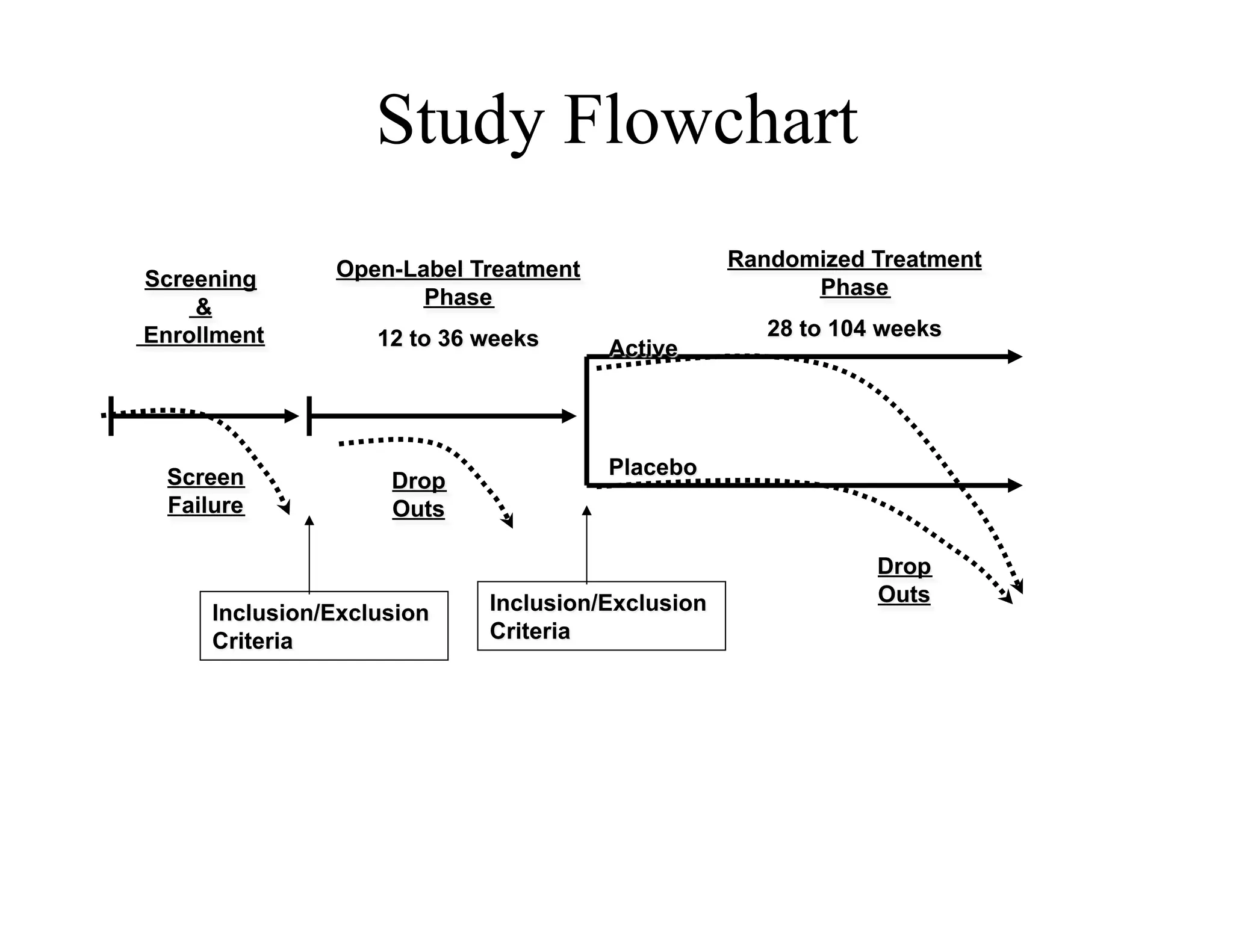
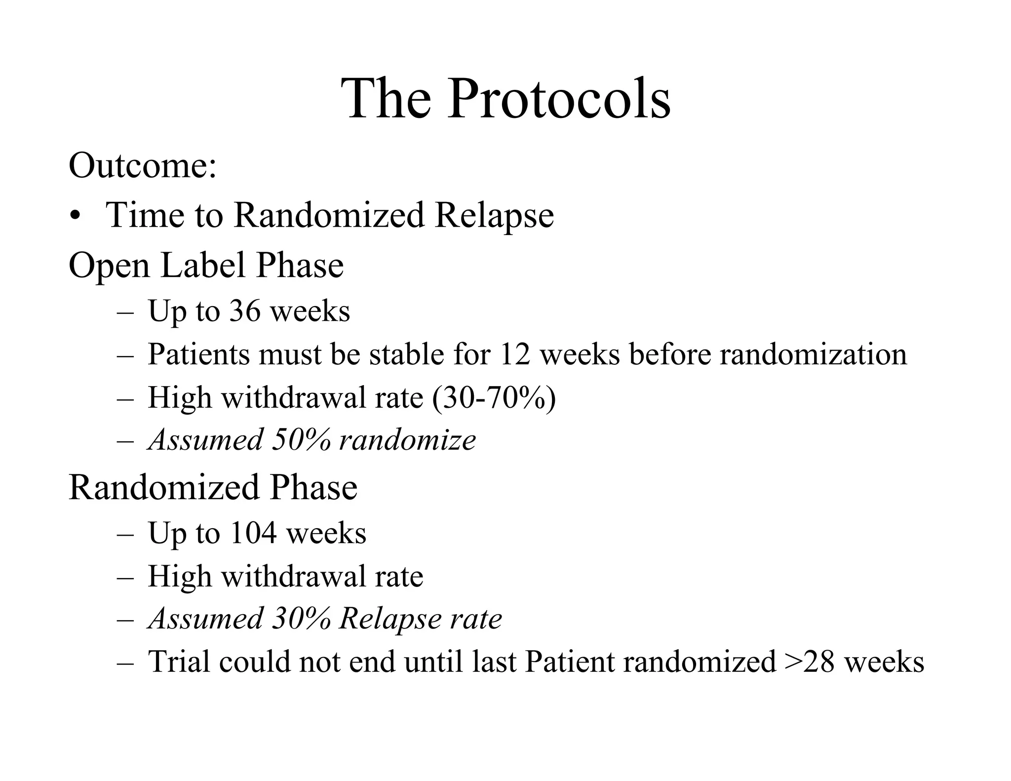
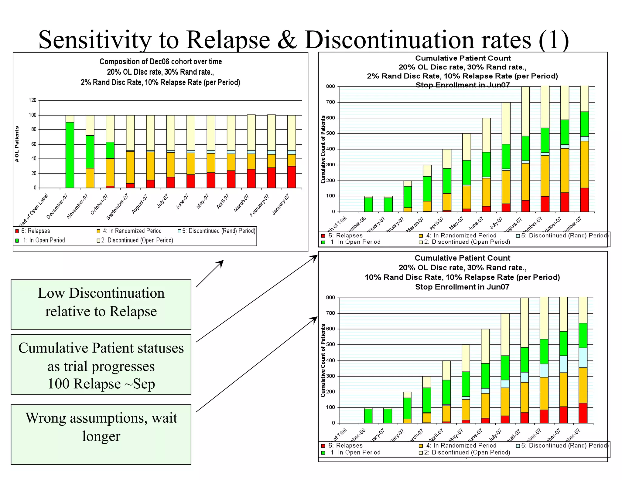
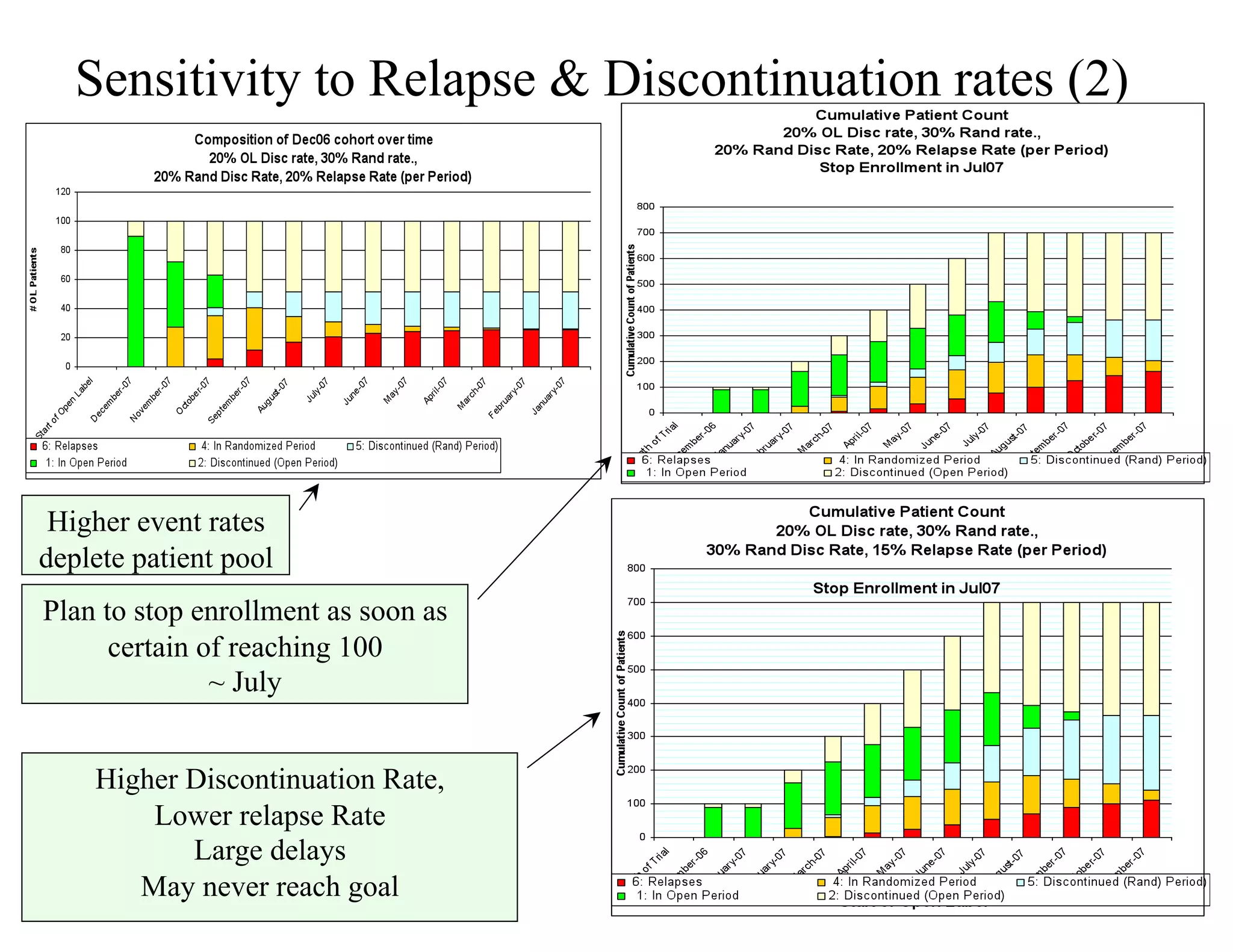
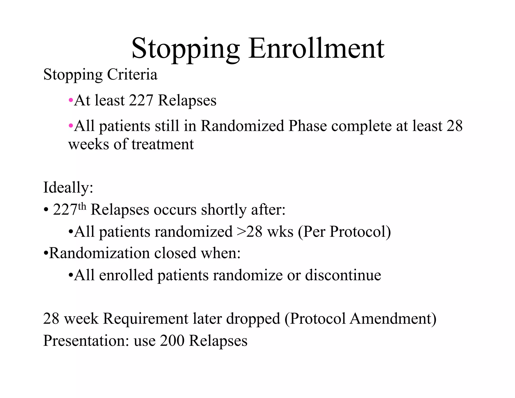
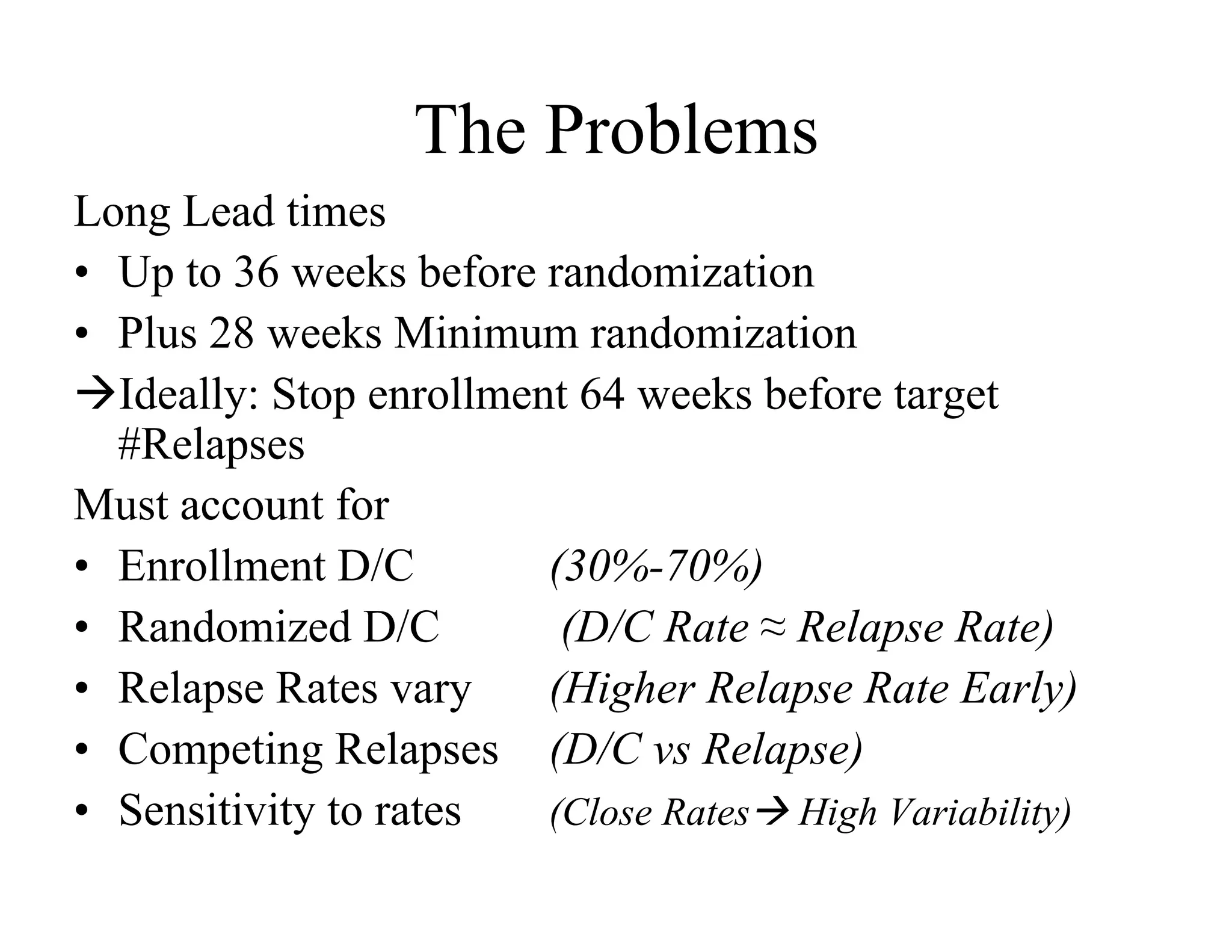
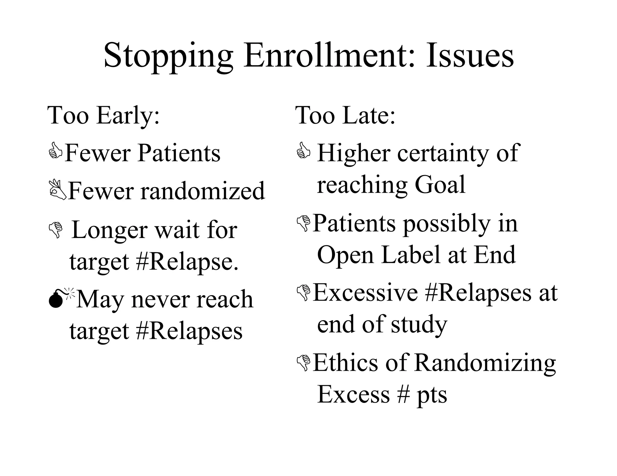
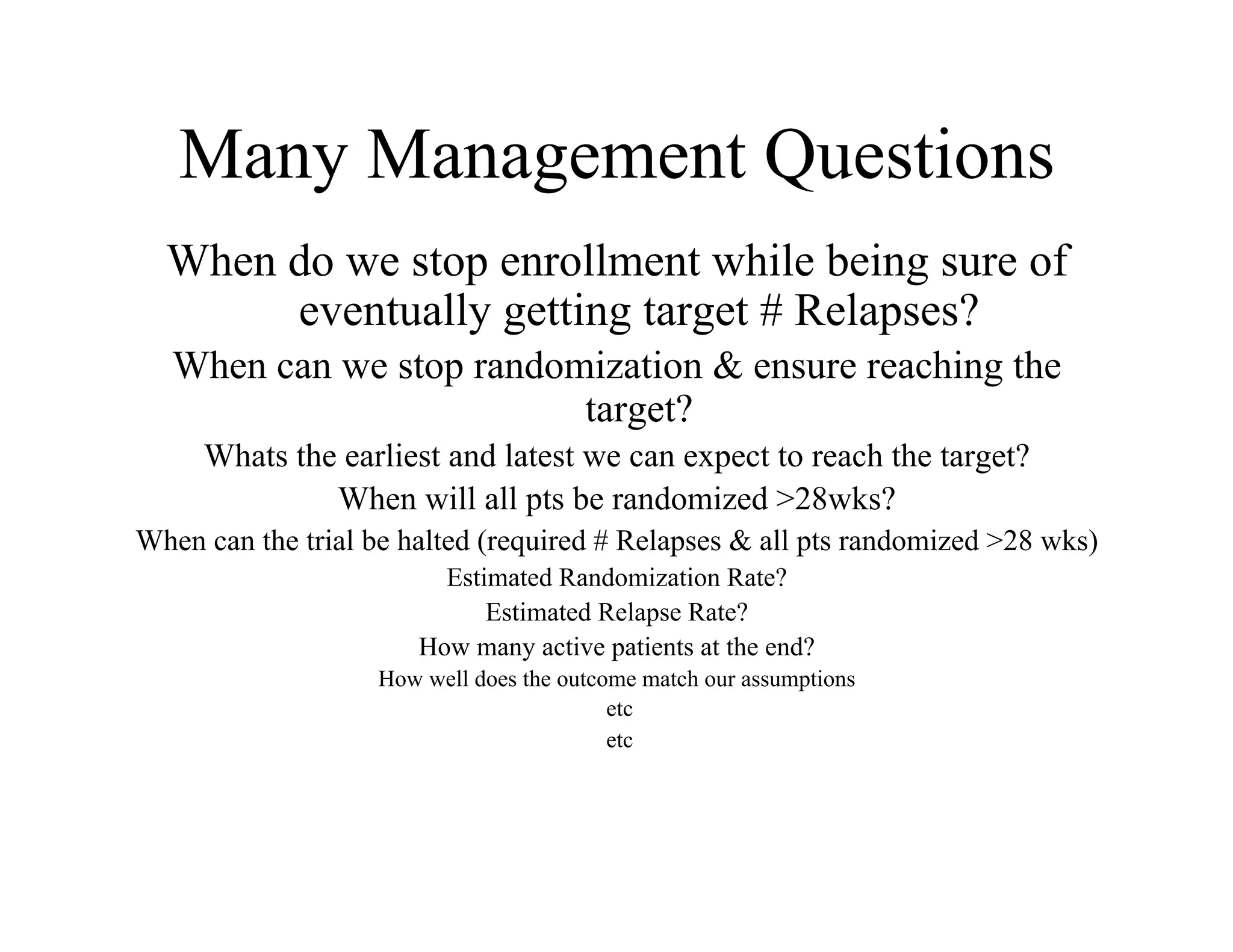
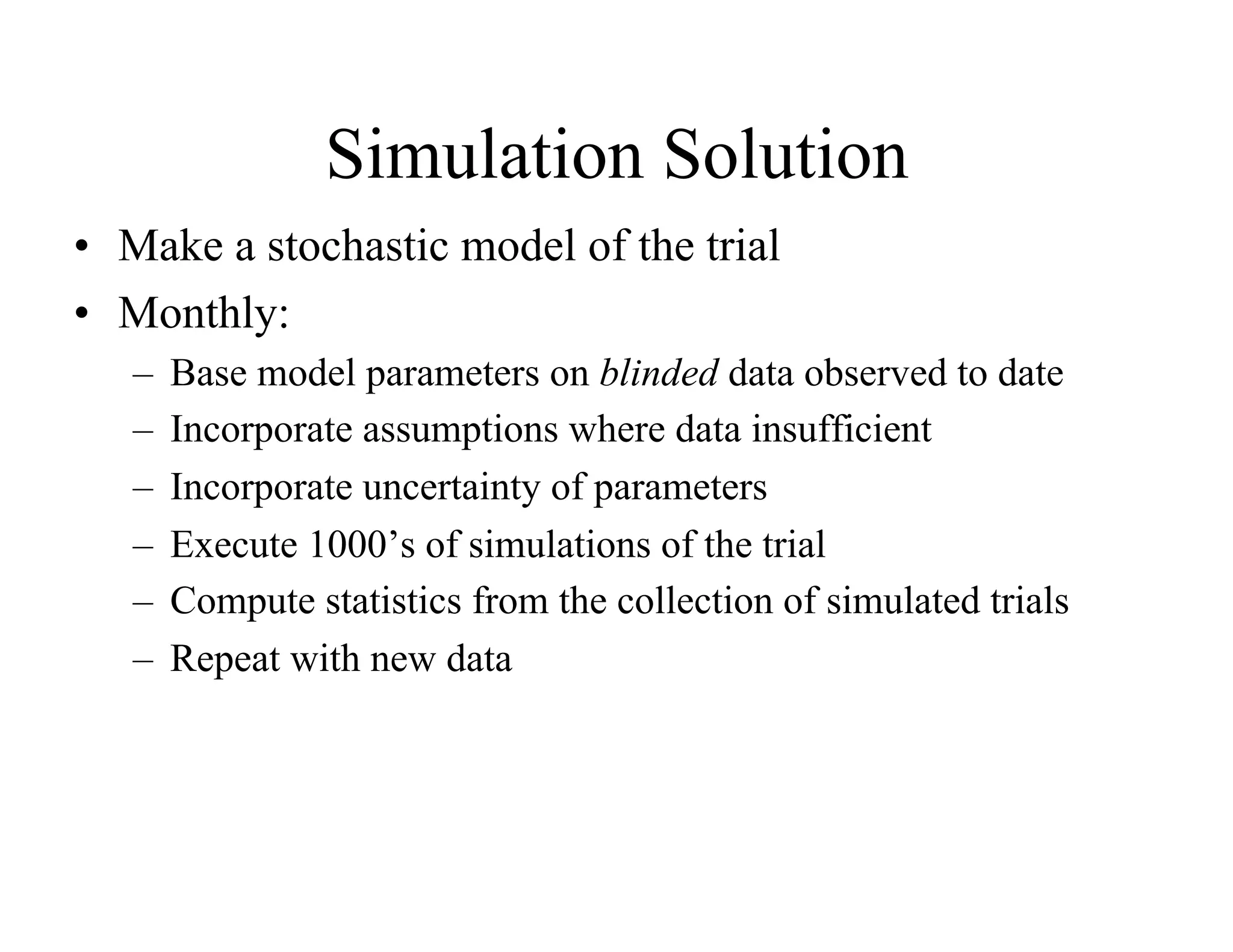
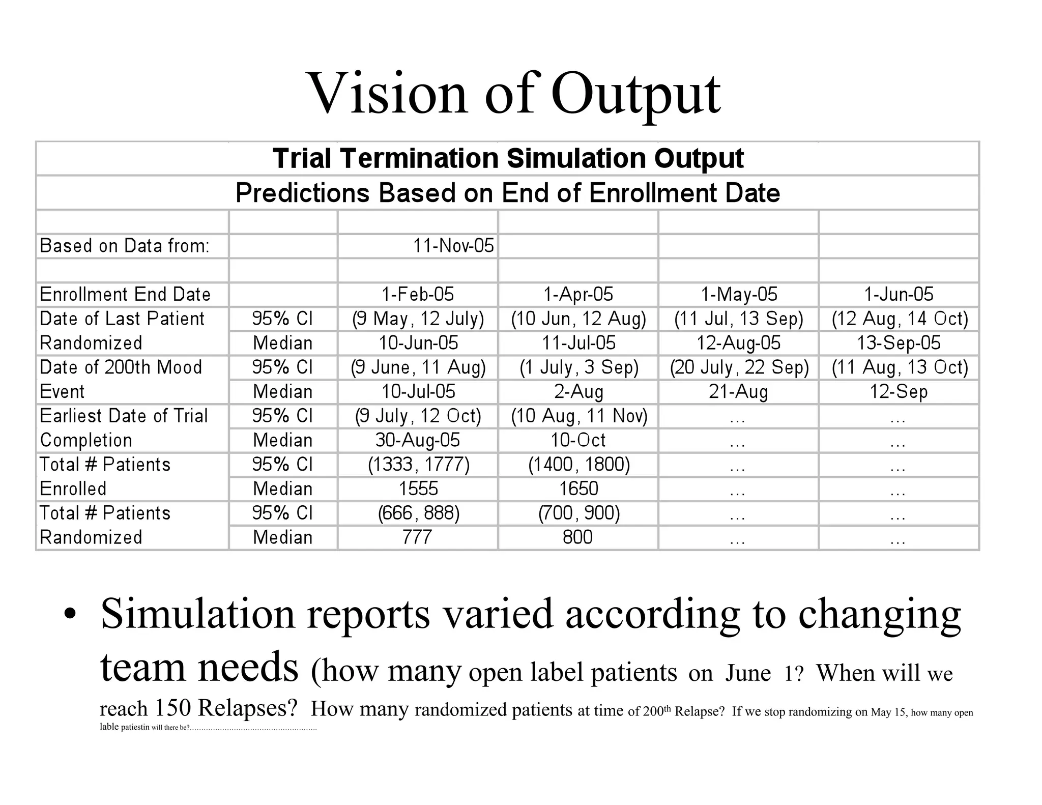
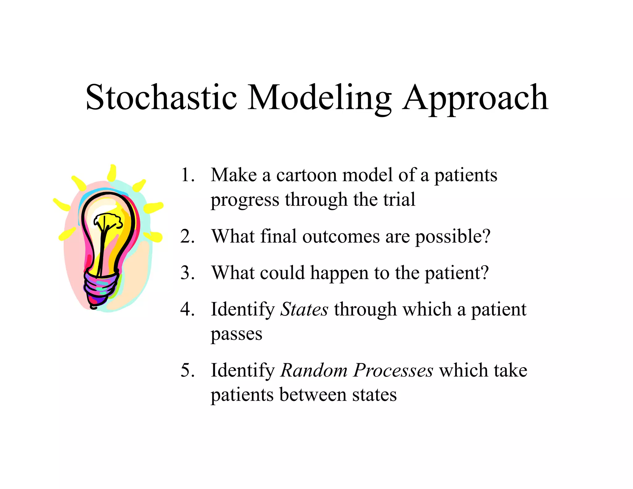

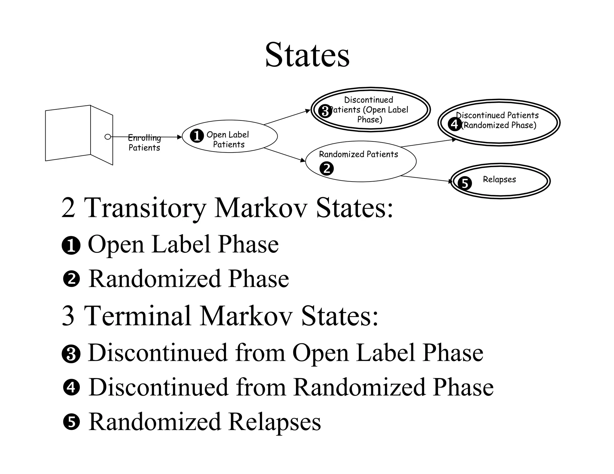
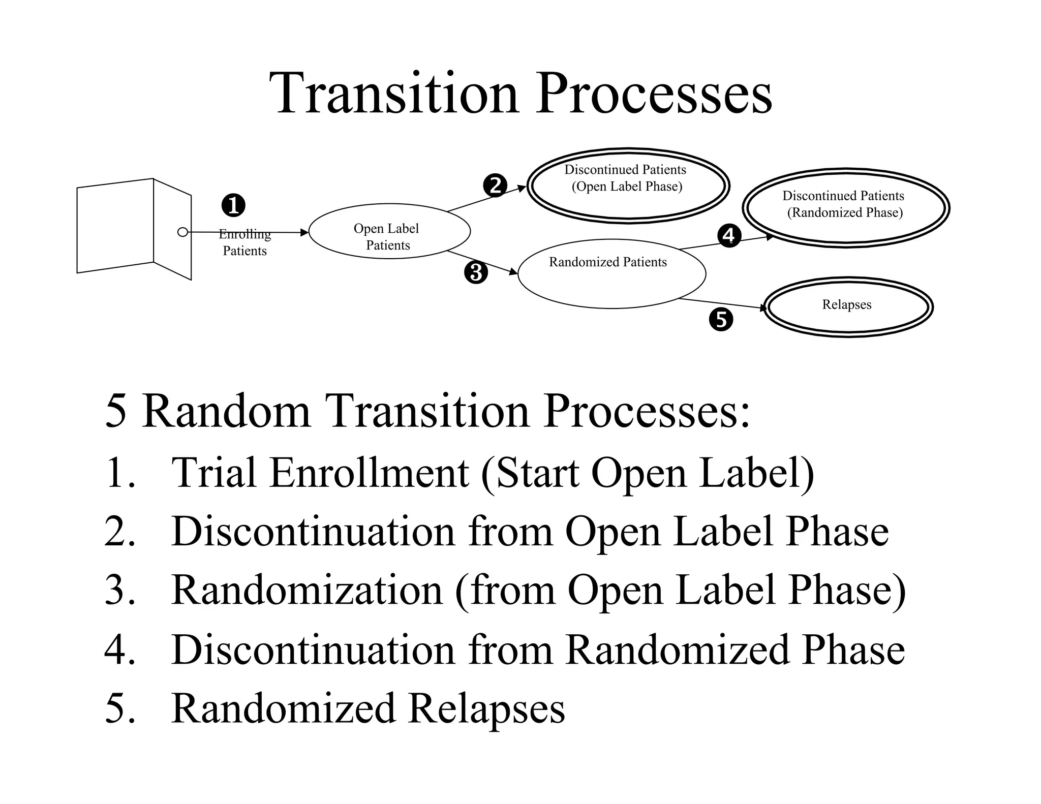
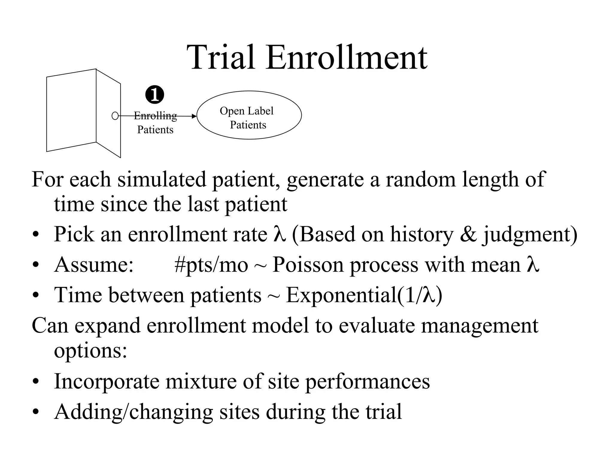
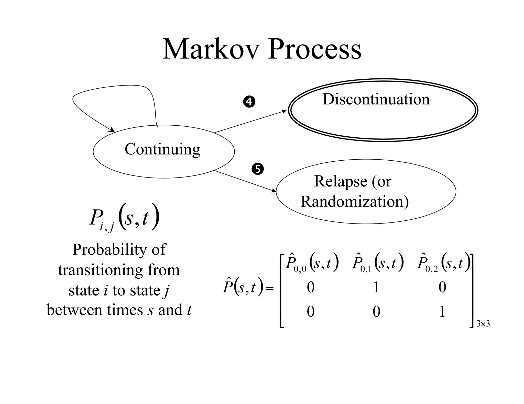

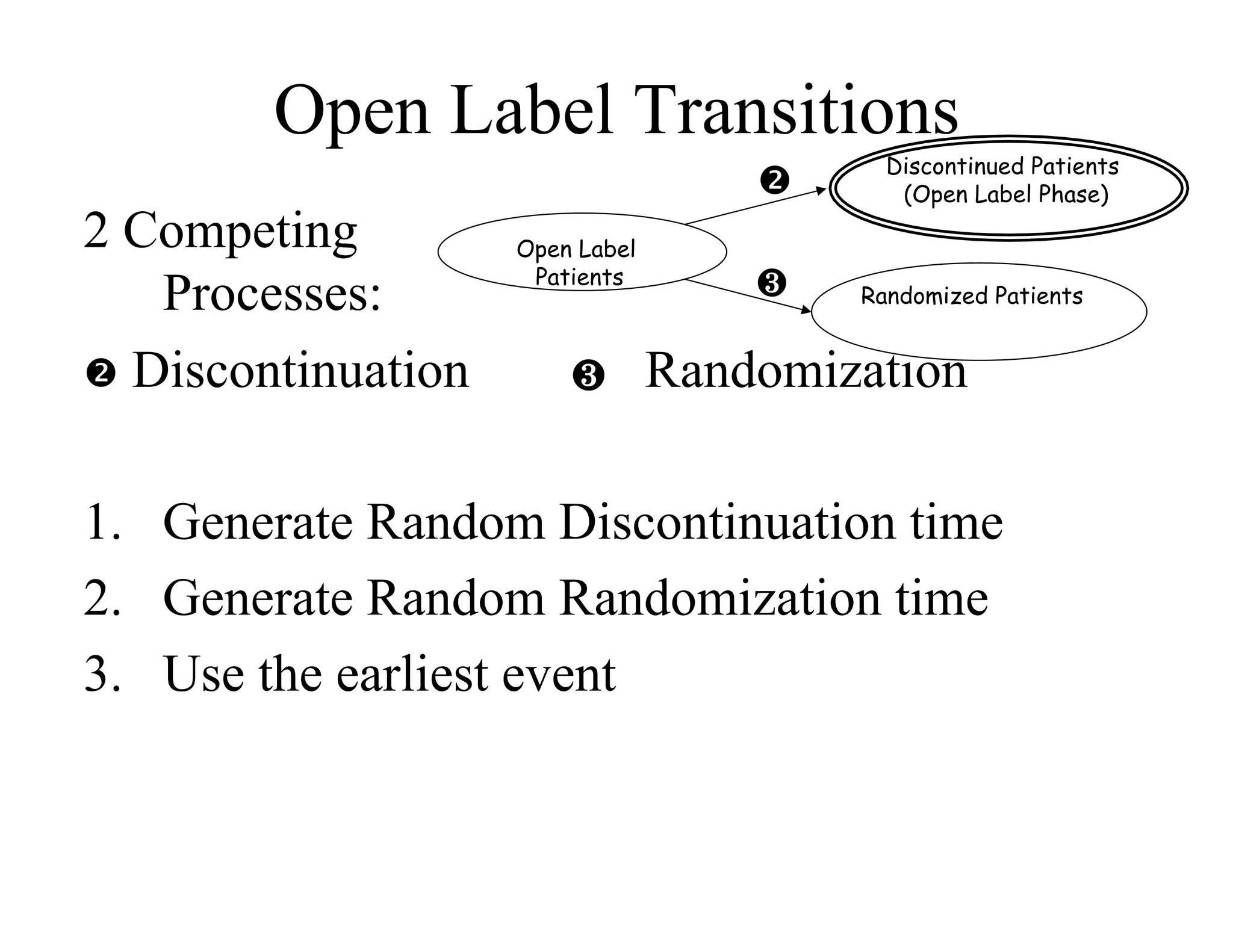
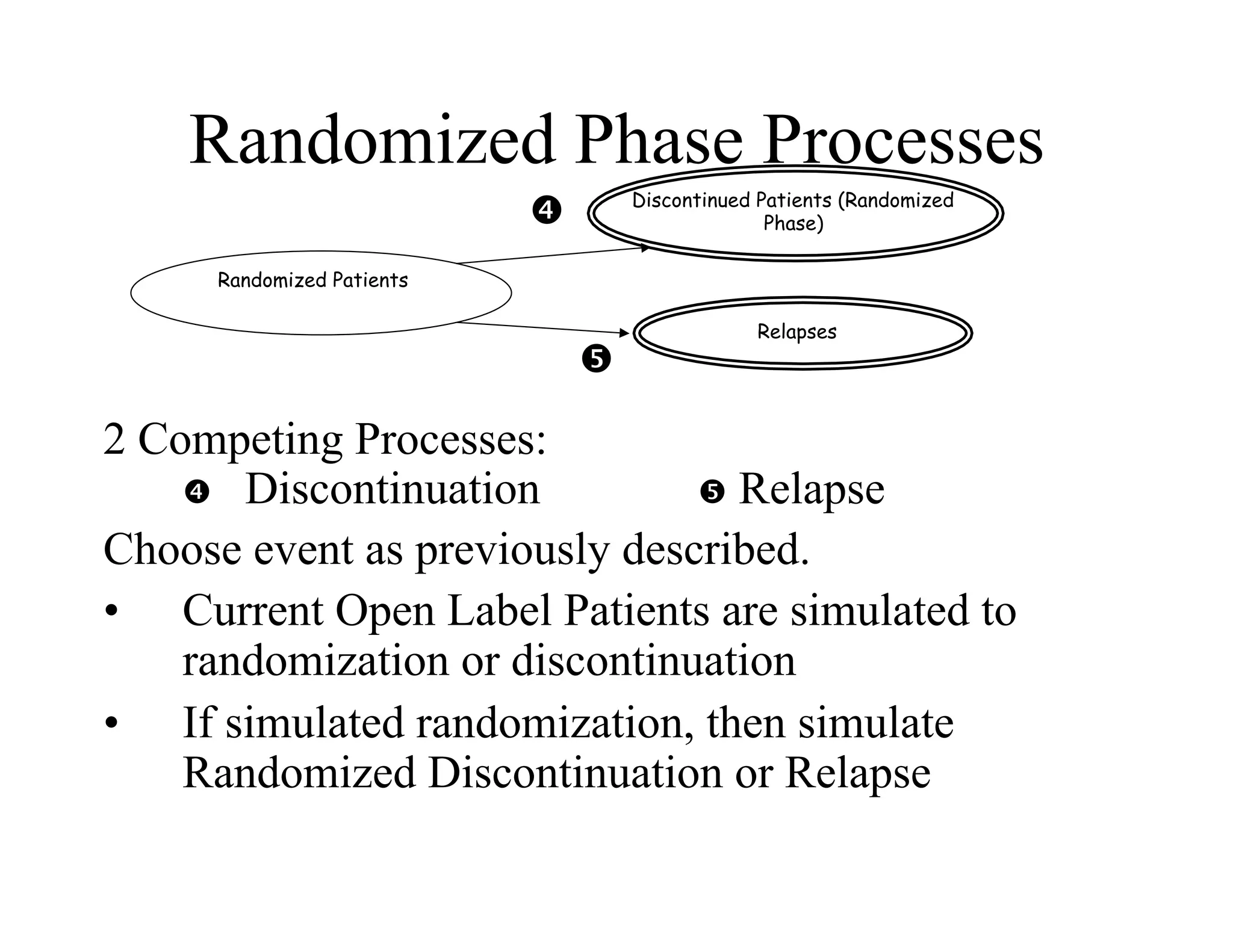
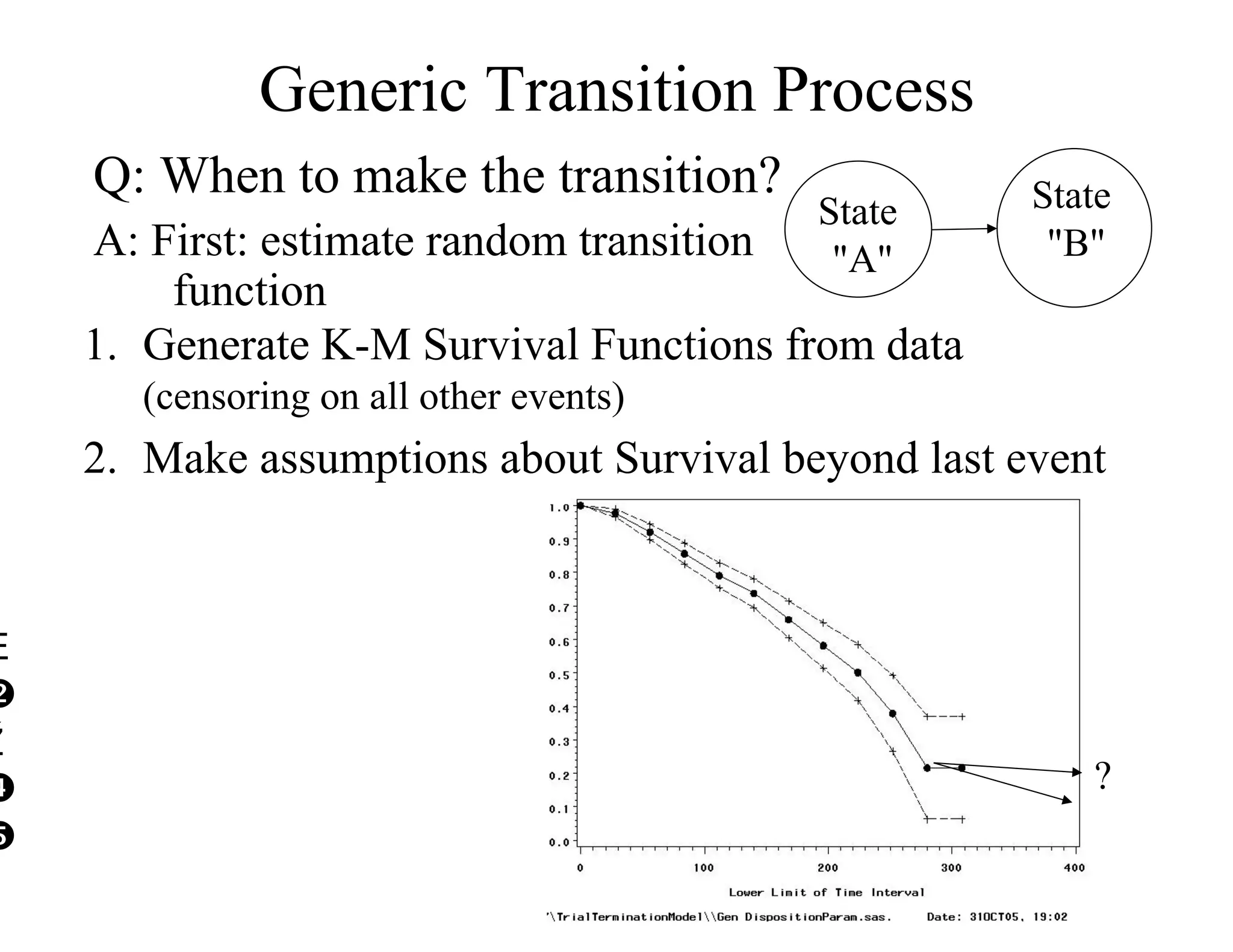
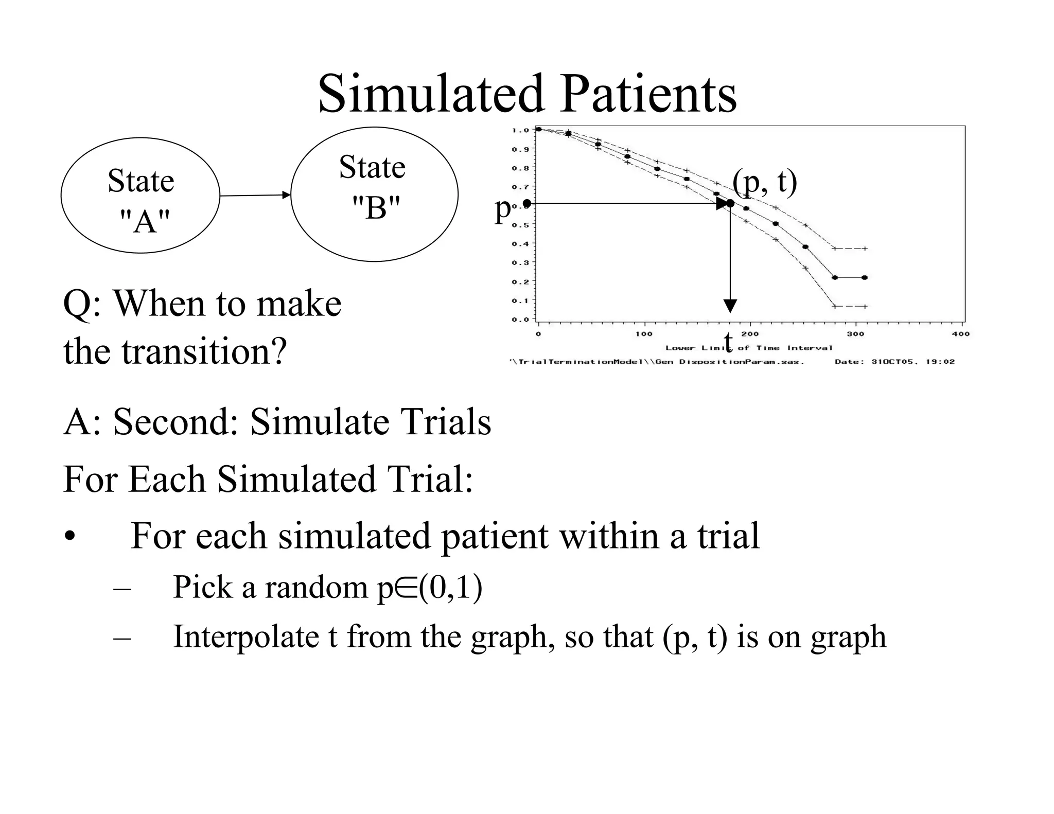
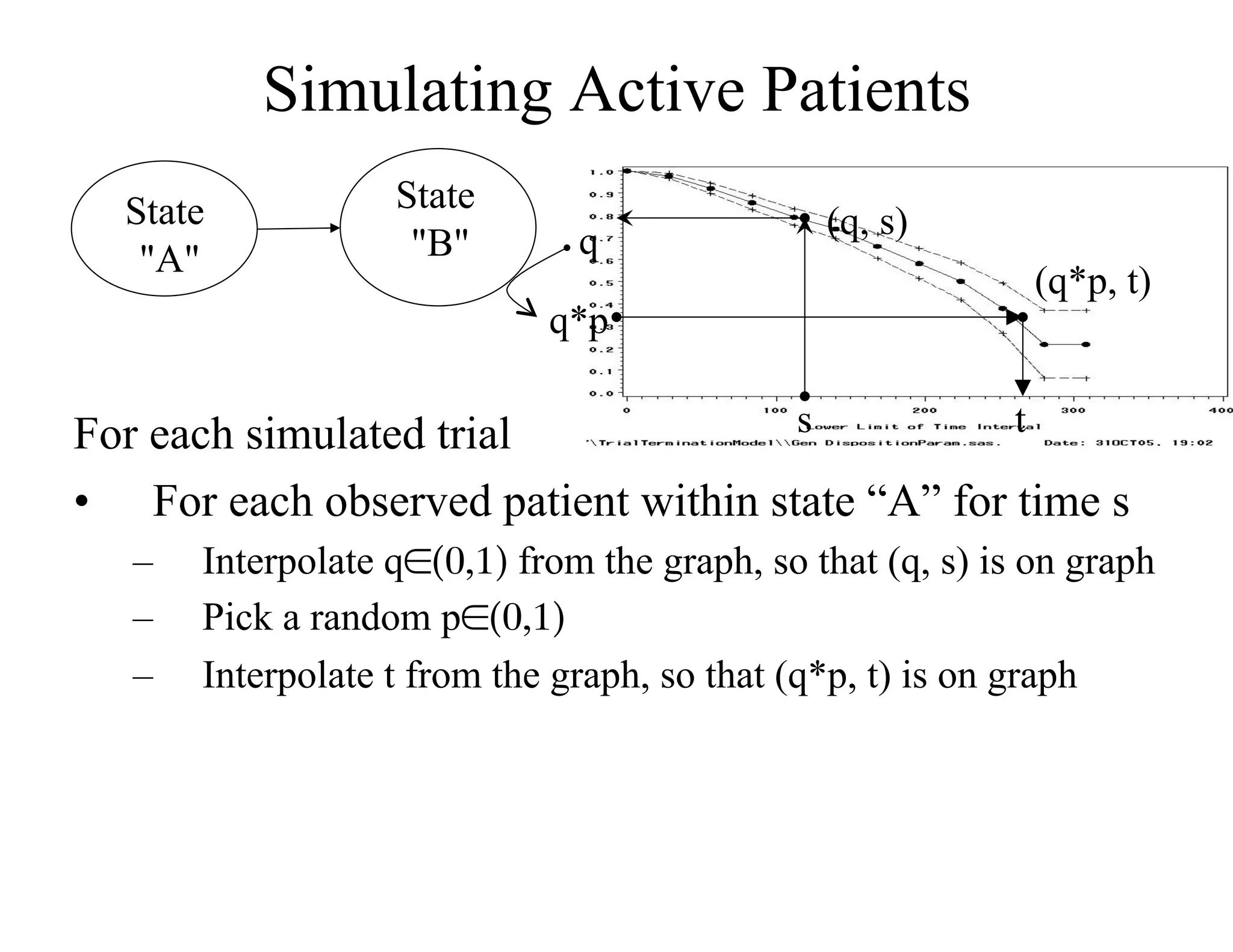
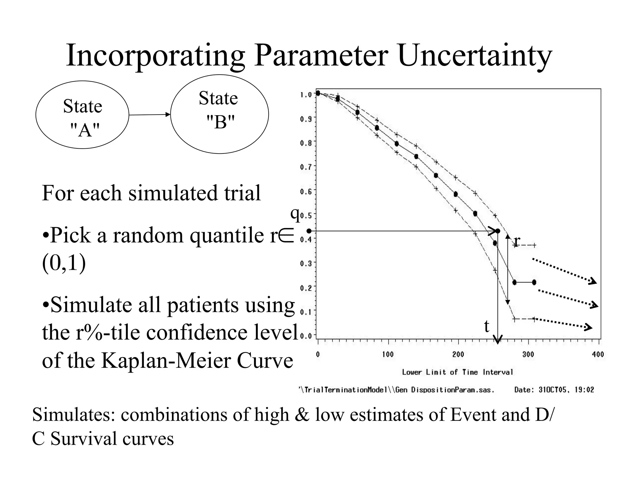
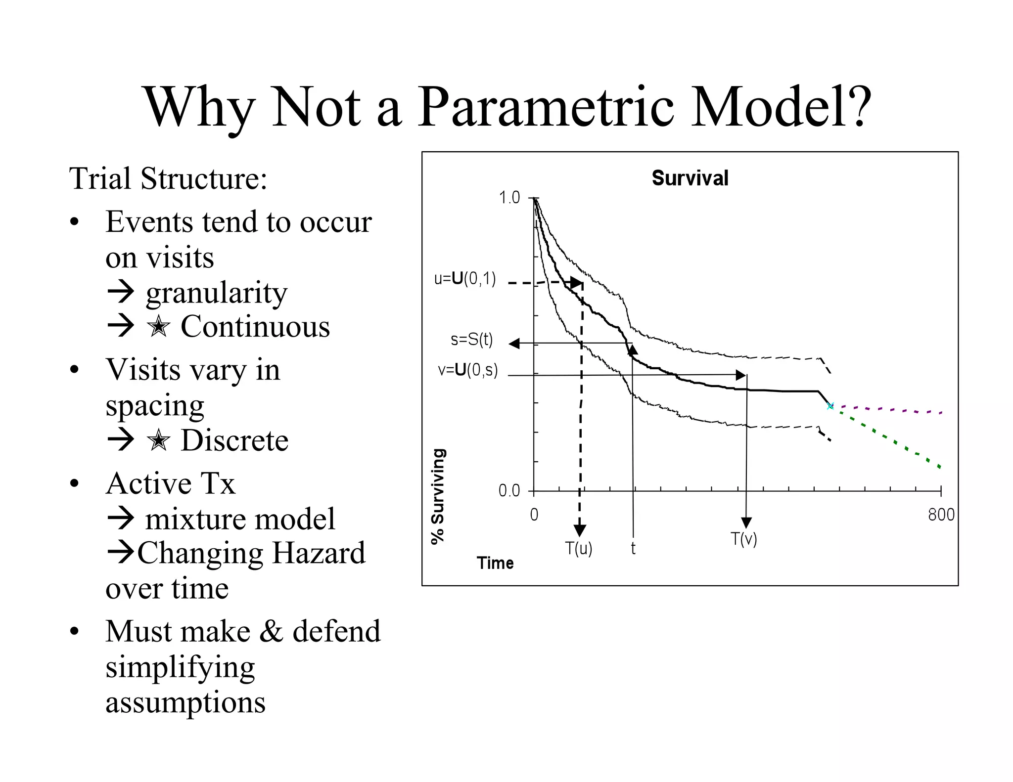
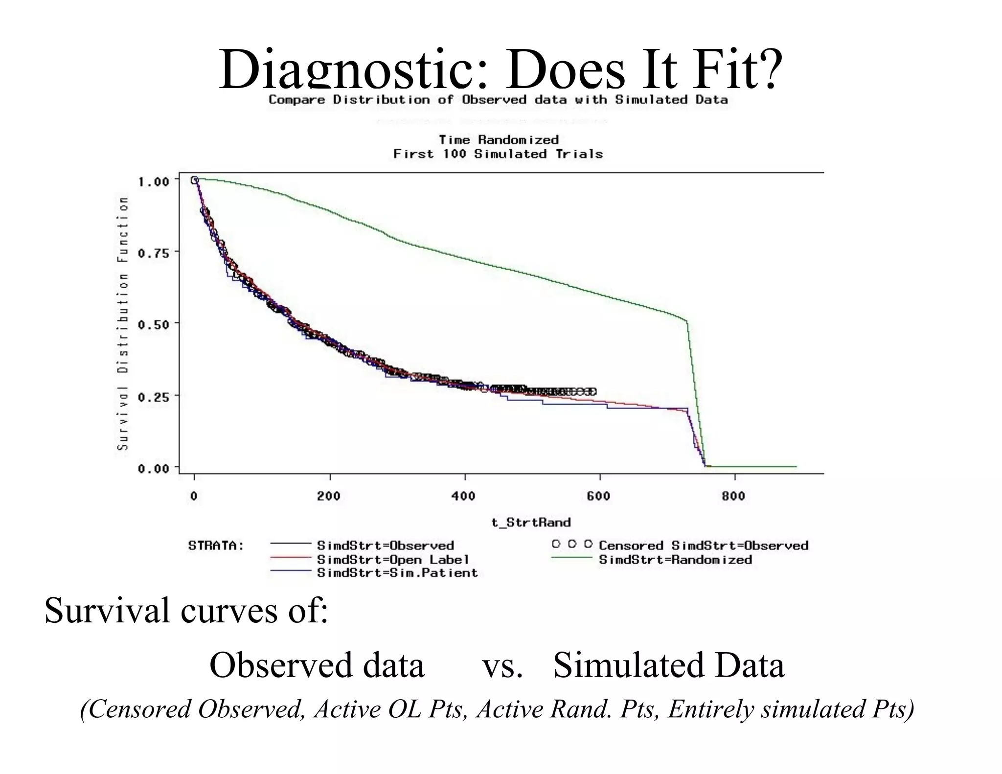
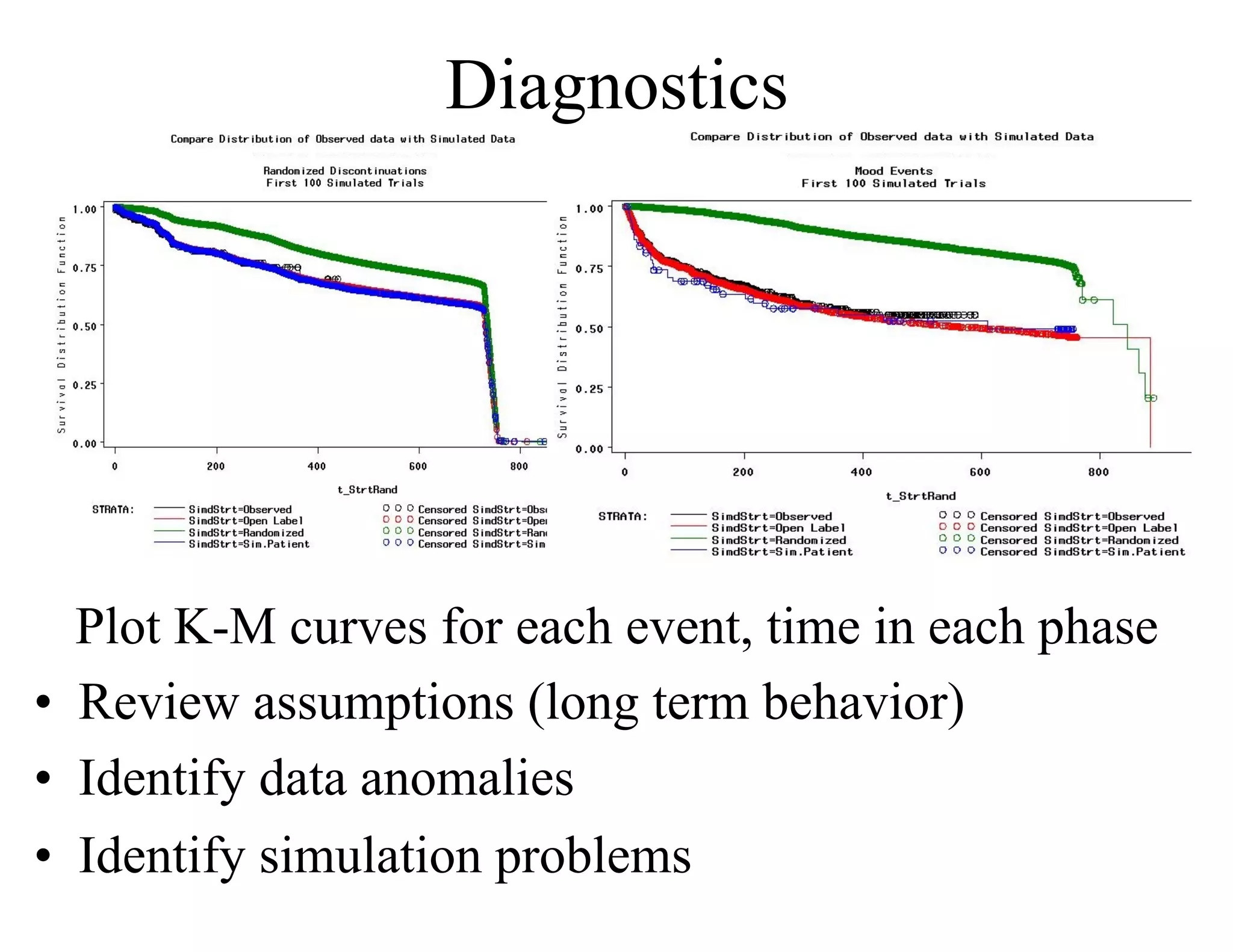
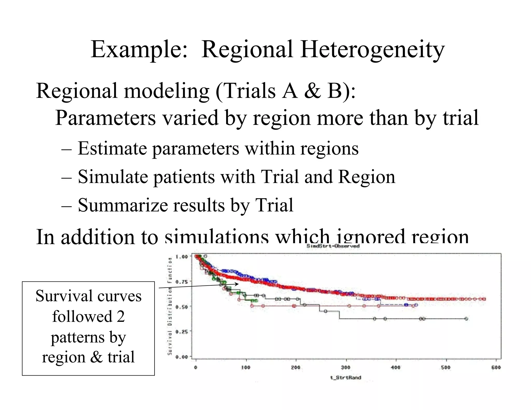
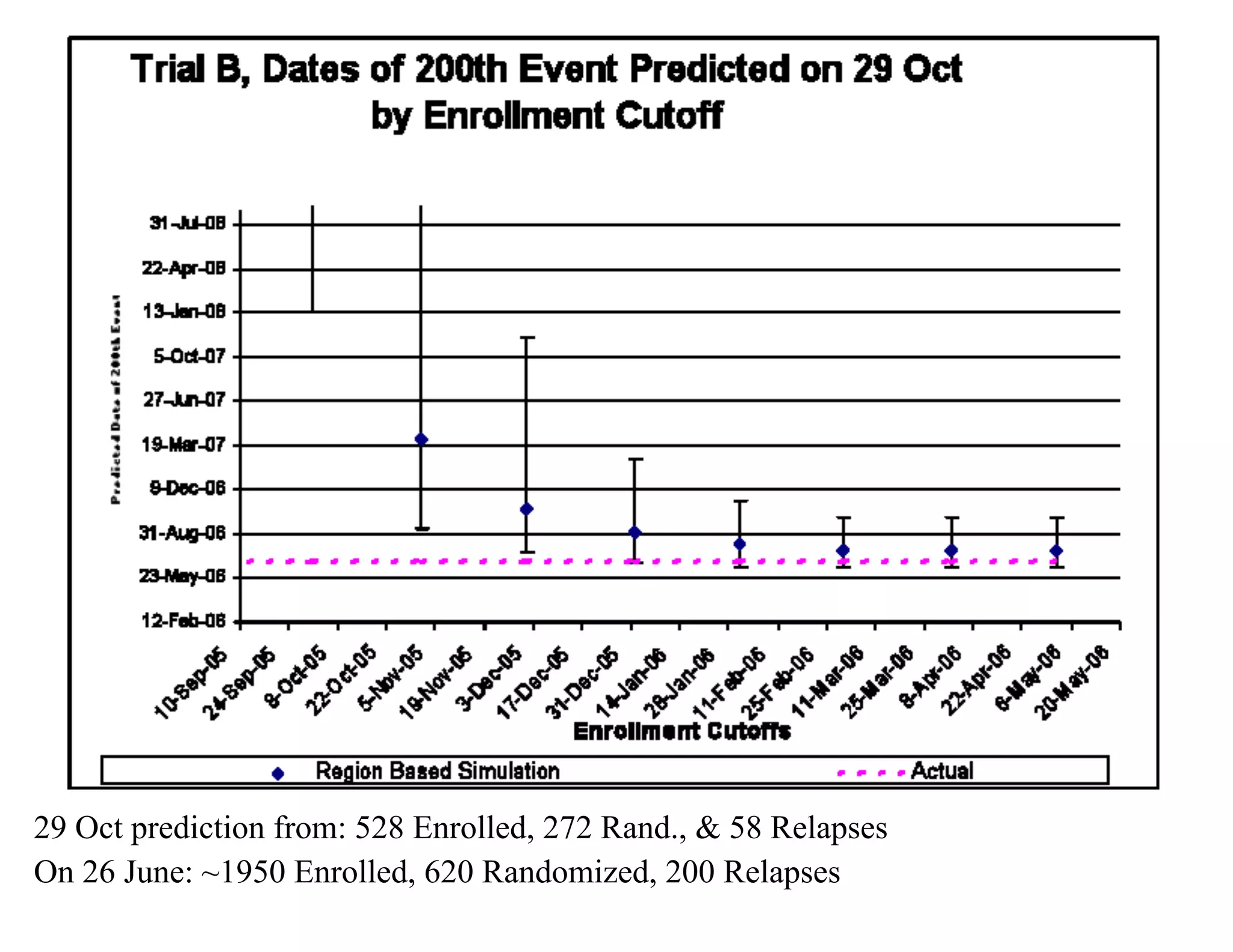
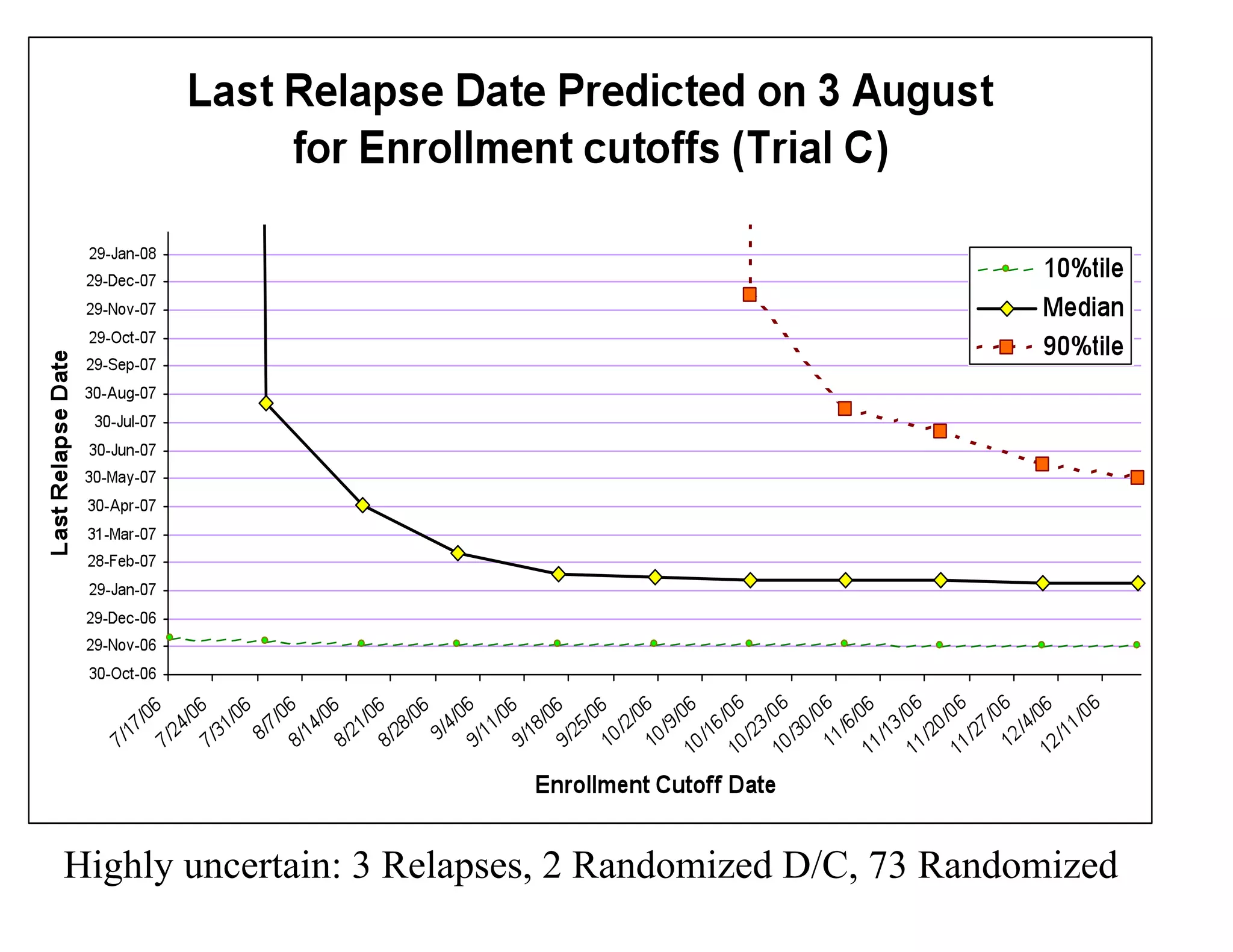
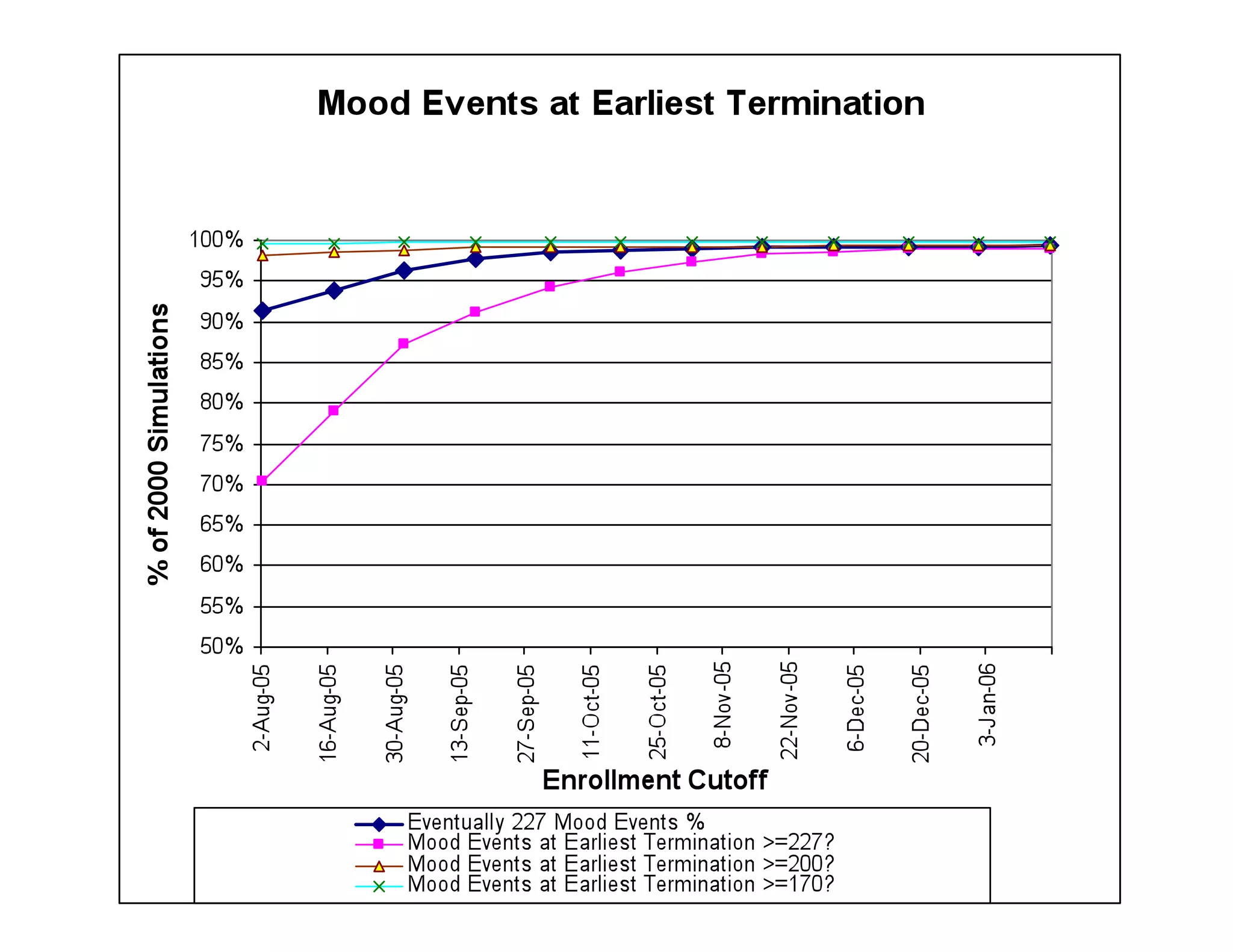
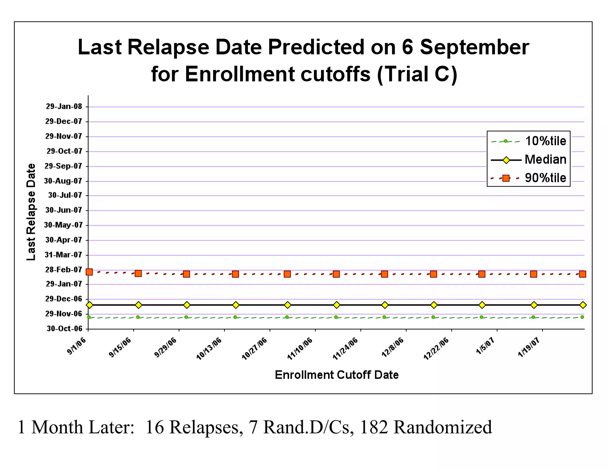
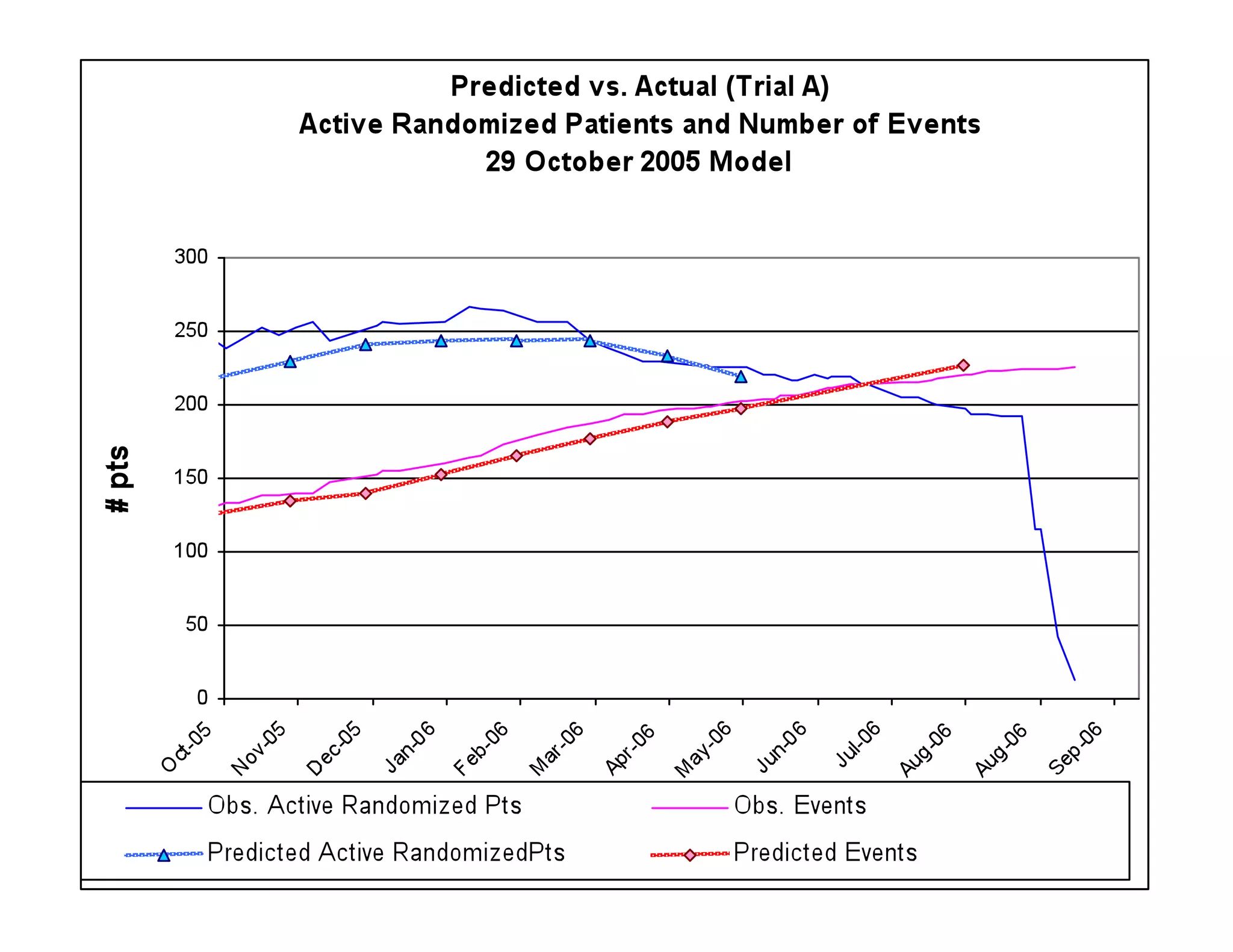
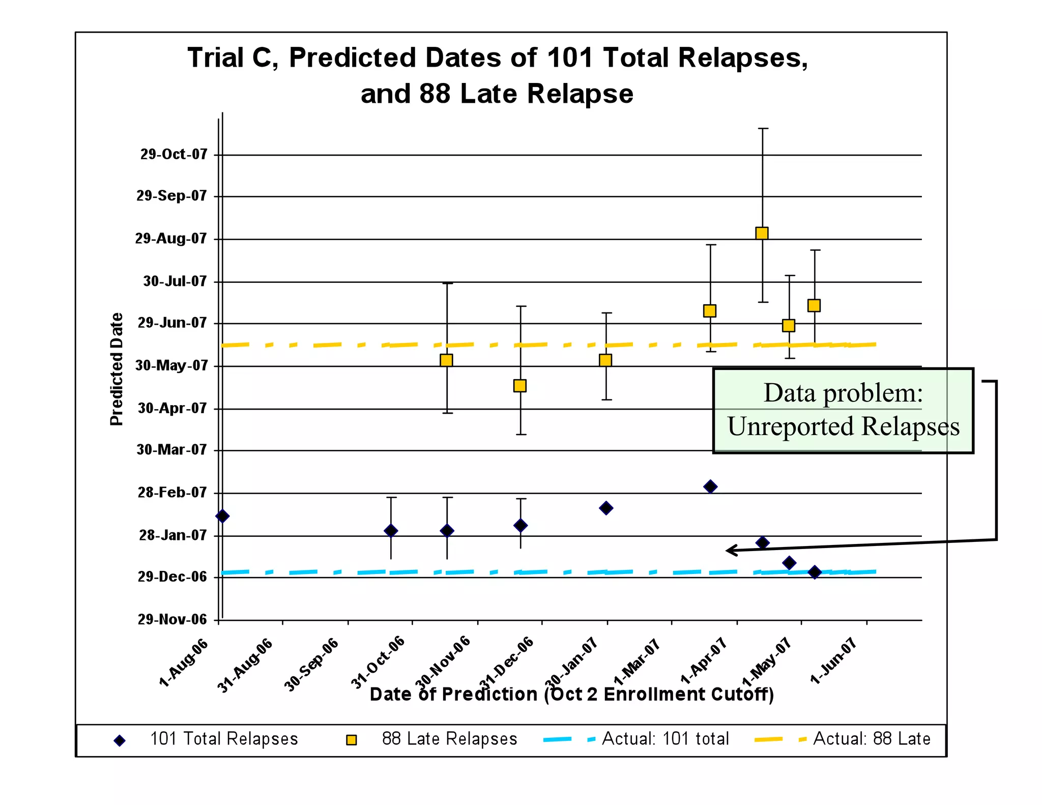
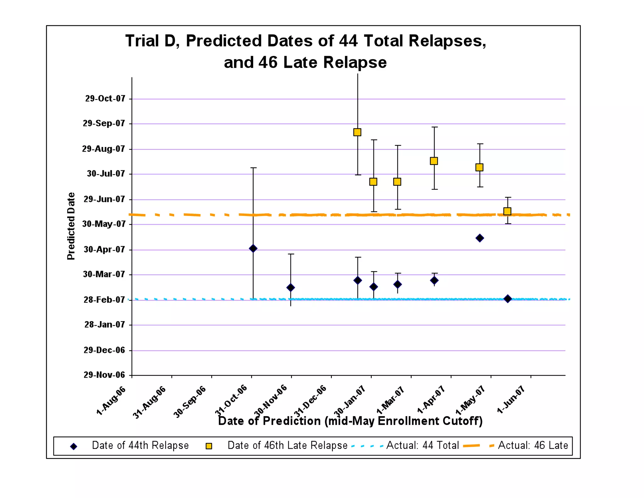
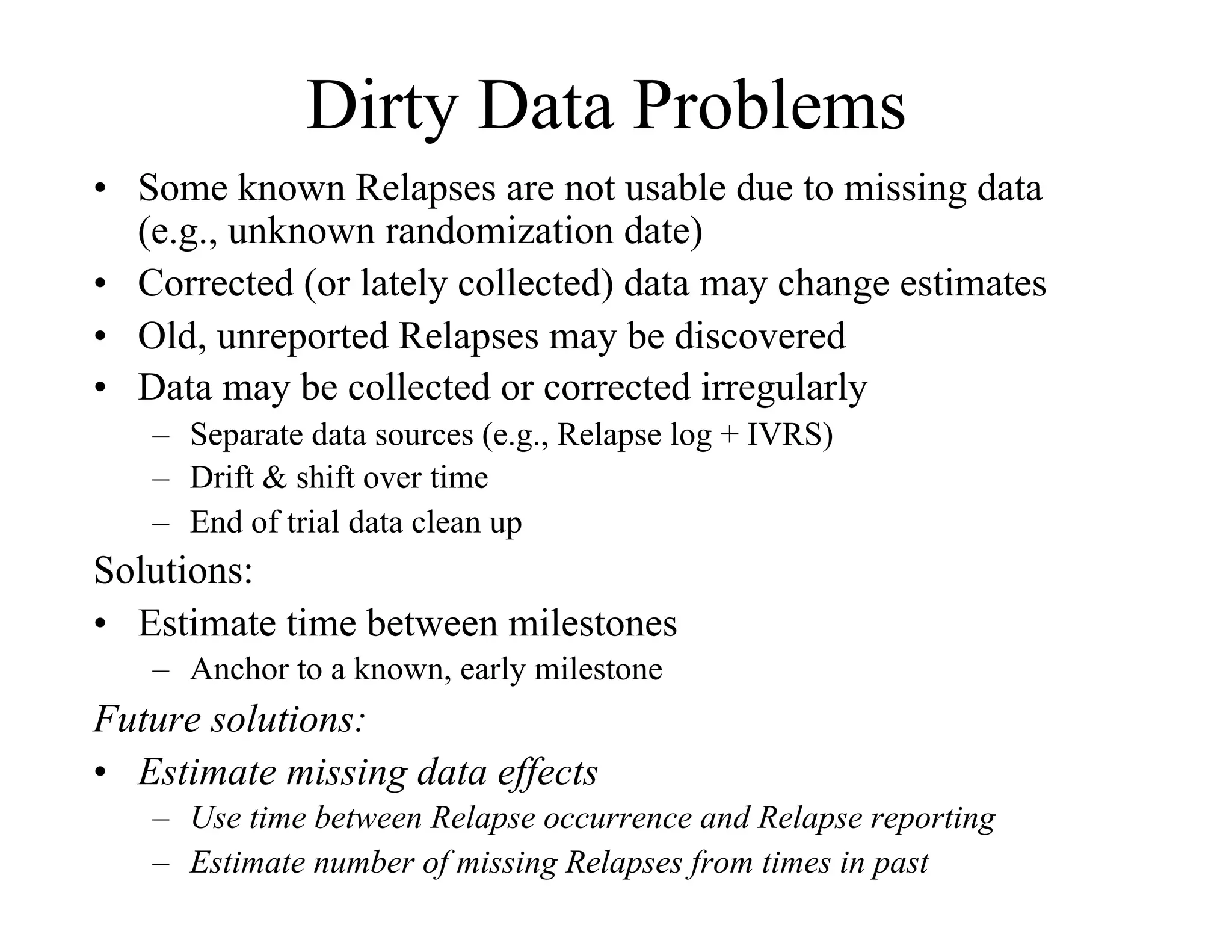
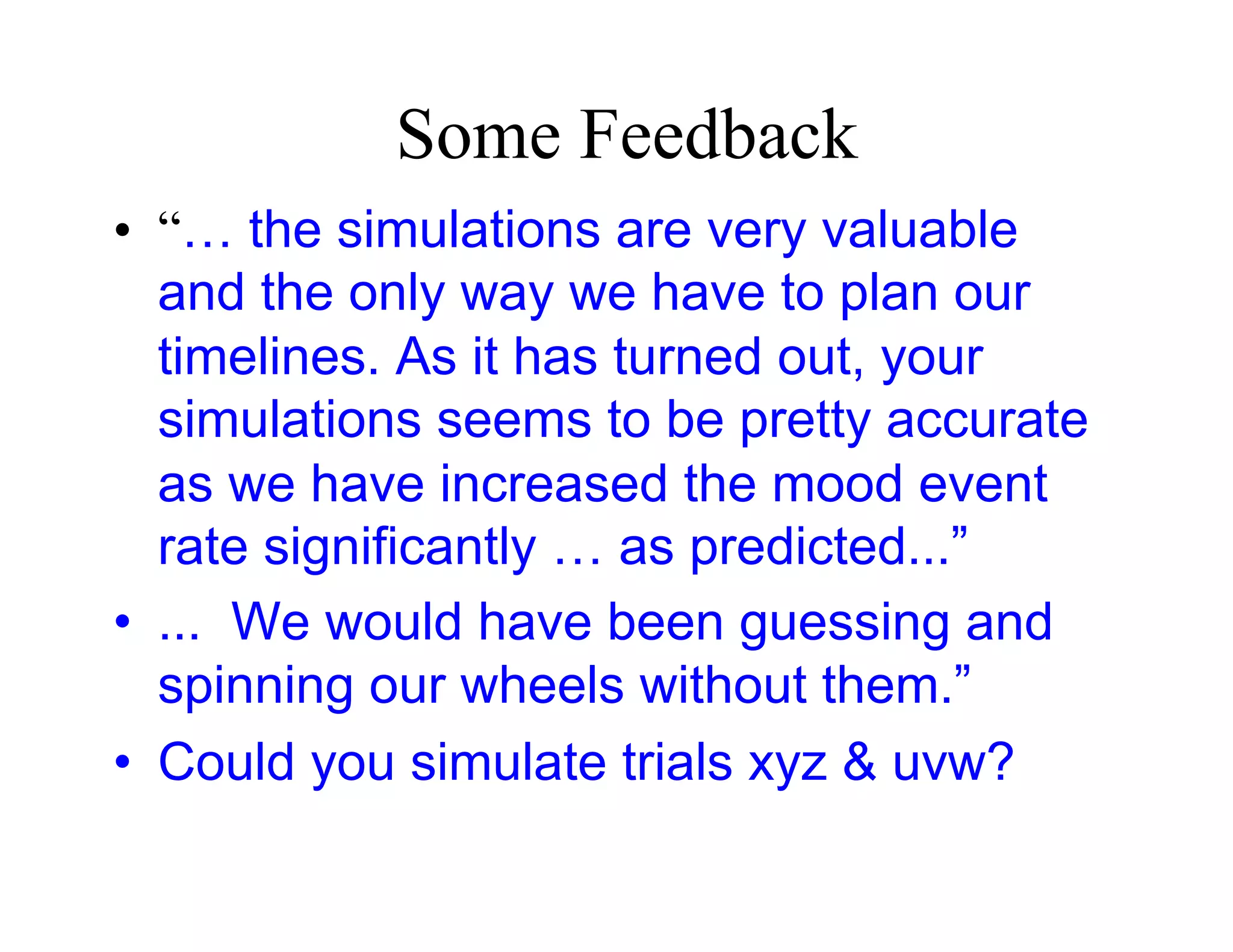

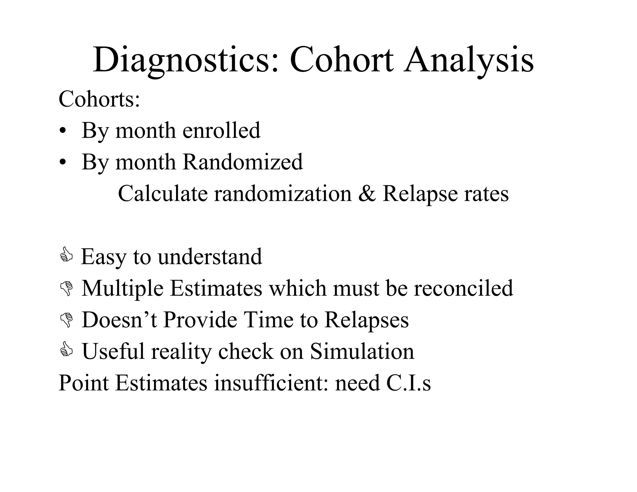
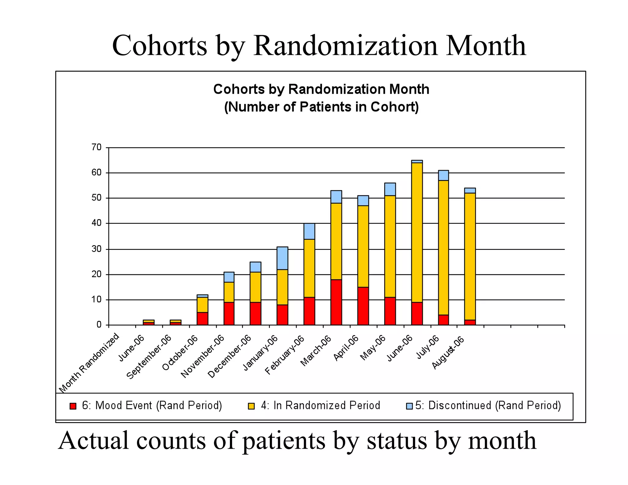
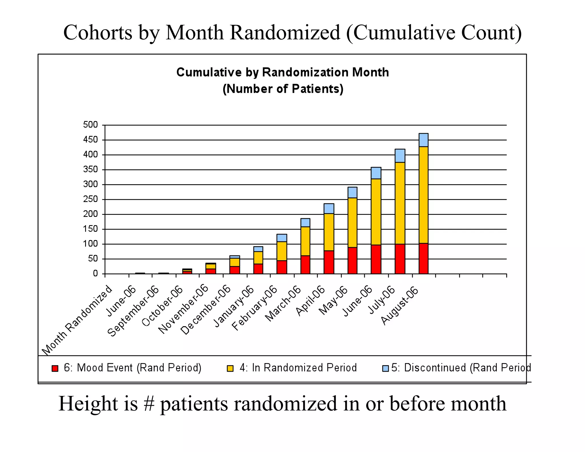

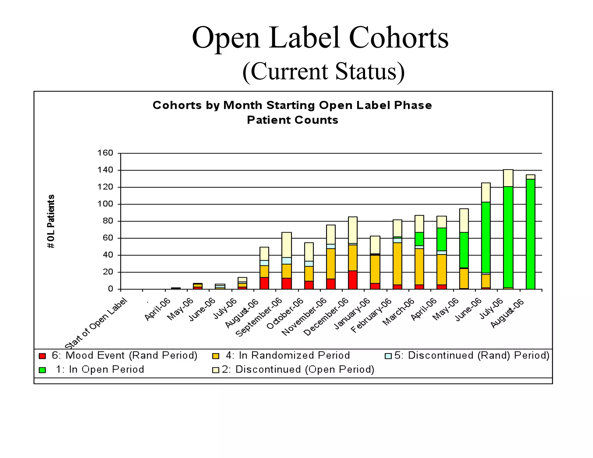
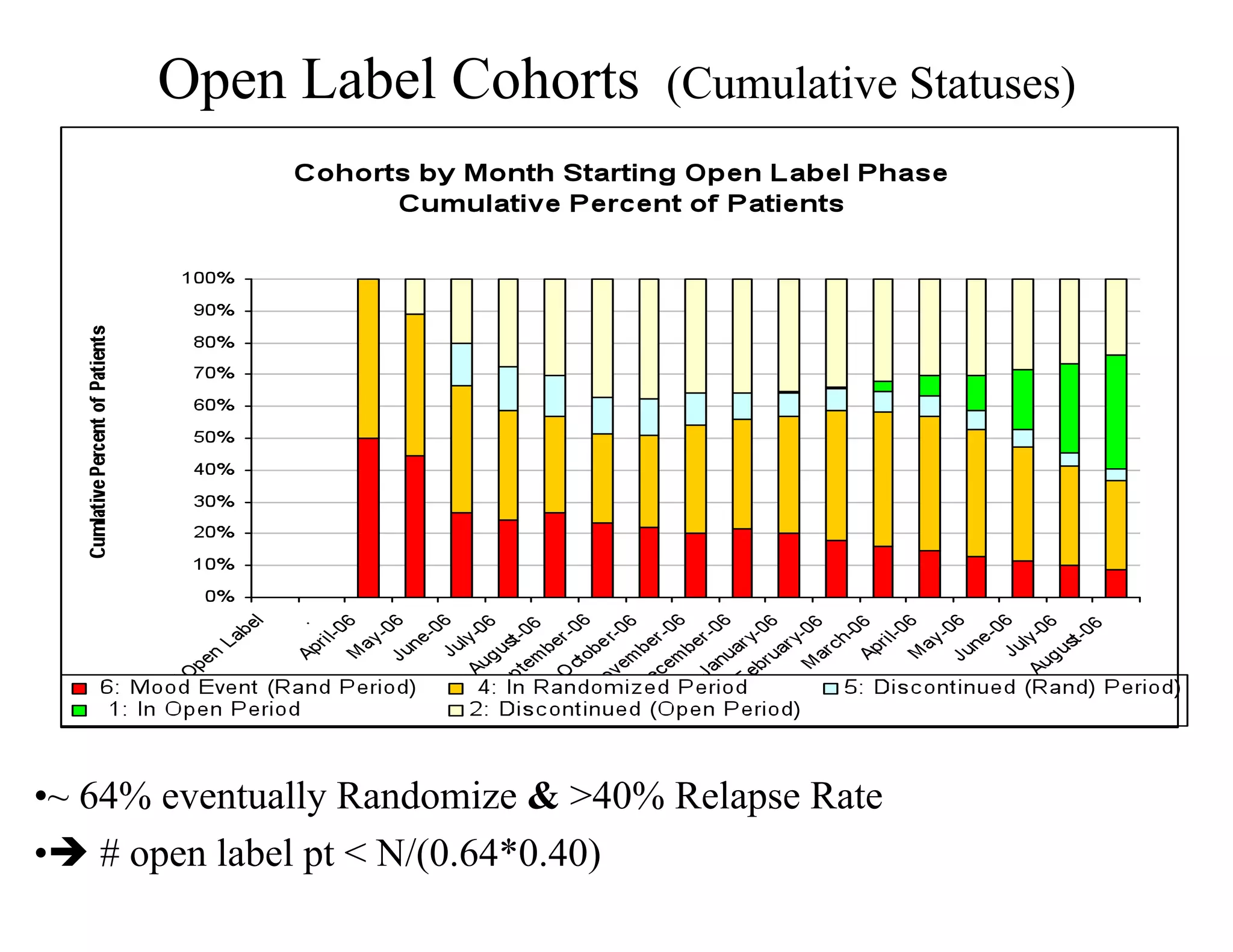

The document discusses the complexities and methodologies in managing multiphase survival trials, particularly focusing on predicting completion times and handling high withdrawal rates. It emphasizes using stochastic modeling to assess patient progression through various trial phases, optimizing enrollment and randomization strategies, and addressing uncertainties related to relapse rates and trial outcomes. Additionally, it outlines the importance of continuous data updating and how simulations can guide trial management decisions effectively.