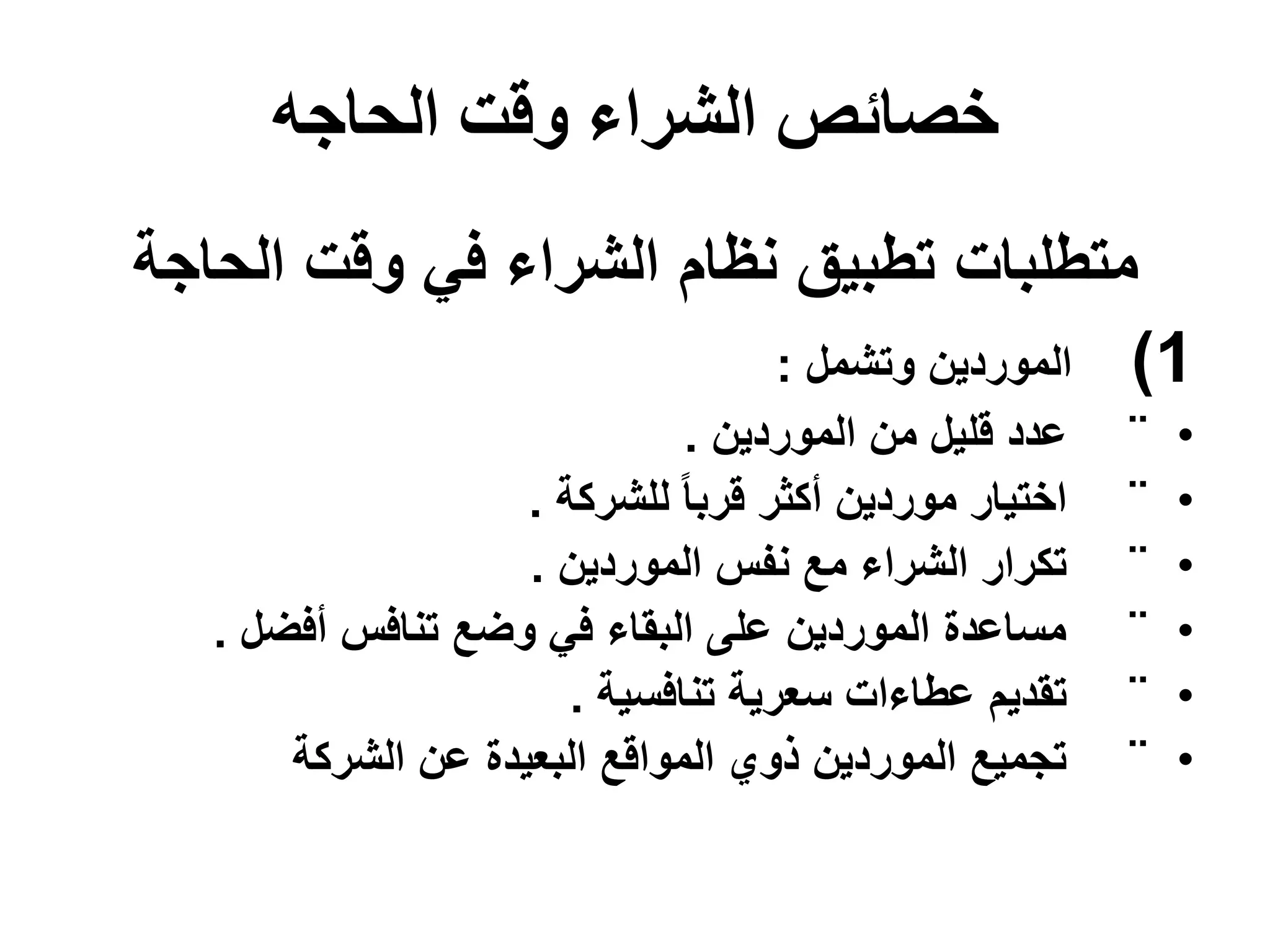
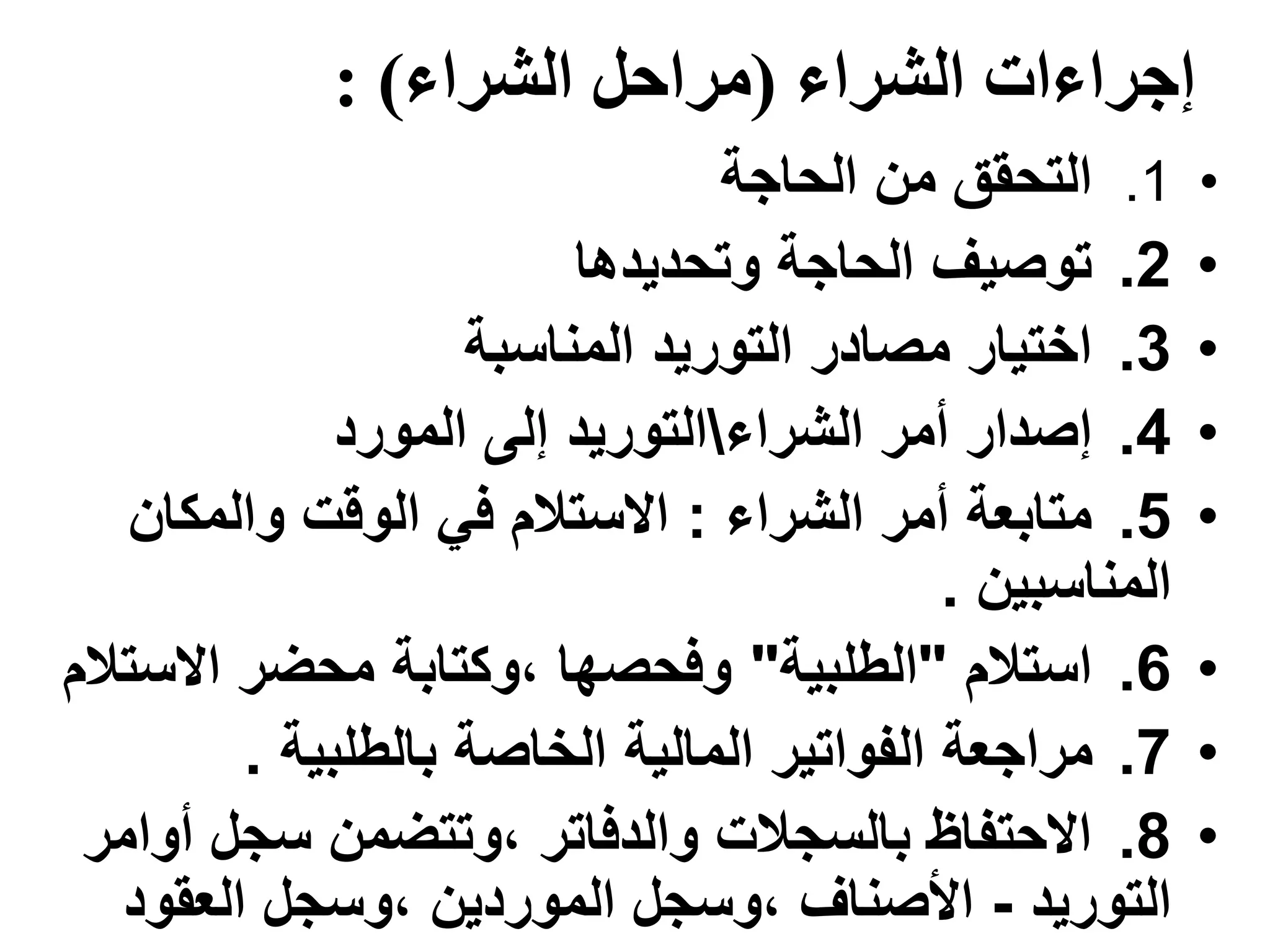
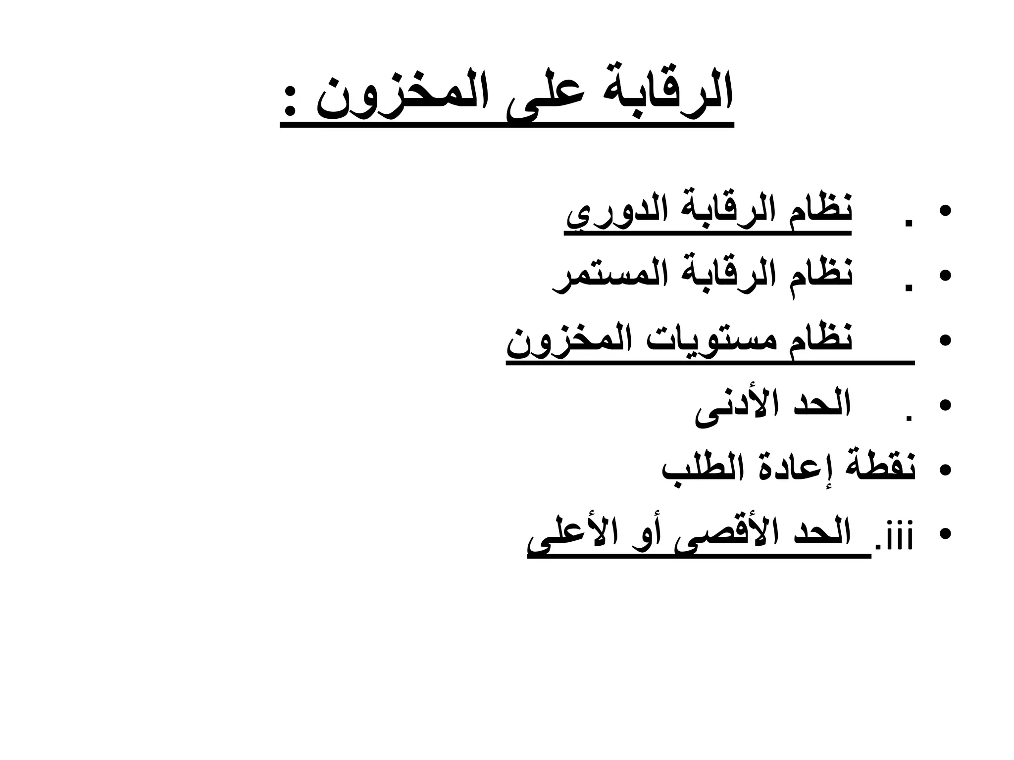
تتناول الوثيقة إدارة الشراء والتمويل وترتكز على أهمية تلبية احتياجات الإنتاج من المواد الخام بشكل فعال. تحدد الوثيقة أيضًا أهداف عملية الشراء مثل تحسين التنافسية وتقليل التكاليف، وتلتزم بإجراءات محددة لجعل عمليات الشراء أكثر دقة وفعالية.
Holding, Ordering, andSetup Costs
Holding costs - the costs of holding or “carrying”
inventory over time
Ordering costs - the costs of placing an order and
receiving goods
Setup costs - cost to prepare a machine or process for
manufacturing an order
77
78.
Holding Costs
Category
Cost (andrange) as a
Percent of Inventory
Value
Housing costs (building rent or depreciation,
operating costs, taxes, insurance)
6% (3 - 10%)
Material handling costs (equipment lease or
depreciation, power, operating cost)
3% (1 - 3.5%)
Labor cost 3% (3 - 5%)
Investment costs (borrowing costs, taxes, and
insurance on inventory)
11% (6 - 24%)
Pilferage, space, and obsolescence 3% (2 - 5%)
Overall carrying cost 26%
78
79.
Holding Costs
Category
Cost (andrange) as a
Percent of Inventory
Value
Housing costs (building rent or depreciation,
operating costs, taxes, insurance)
6% (3 - 10%)
Material handling costs (equipment lease or
depreciation, power, operating cost)
3% (1 - 3.5%)
Labor cost 3% (3 - 5%)
Investment costs (borrowing costs, taxes, and
insurance on inventory)
11% (6 - 24%)
Pilferage, space, and obsolescence 3% (2 - 5%)
Overall carrying cost 26%
79
80.
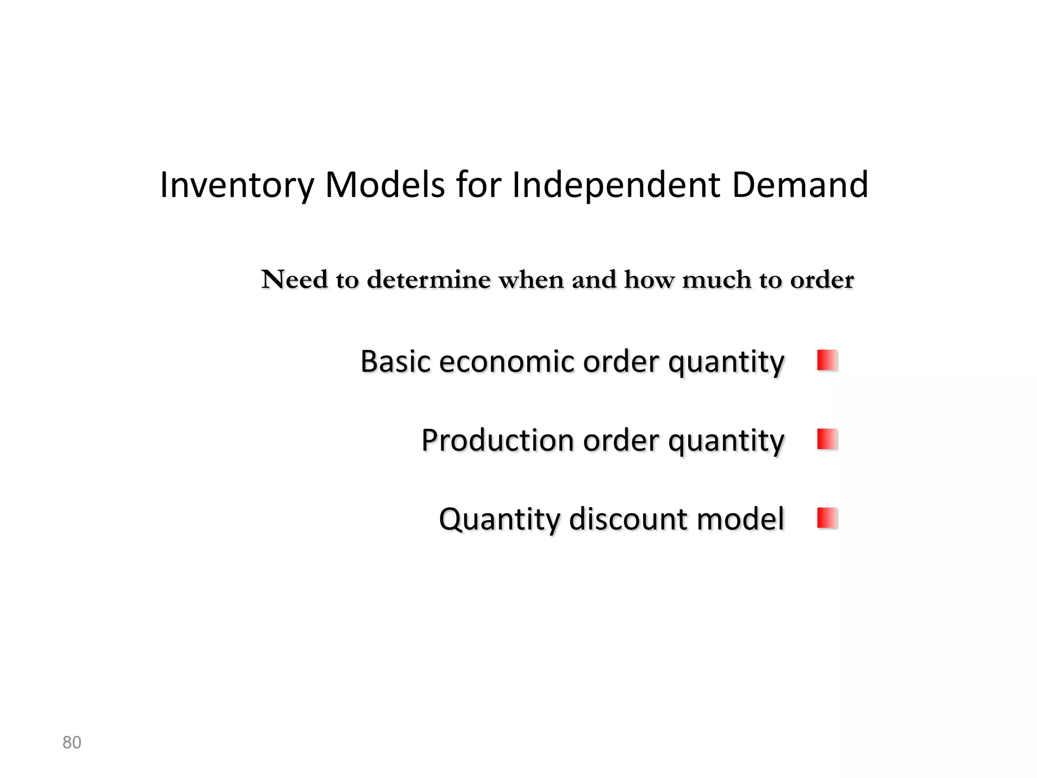
Inventory Models forIndependent Demand
Basic economic order quantity
Production order quantity
Quantity discount model
Need to determine when and how much to order
80
81.
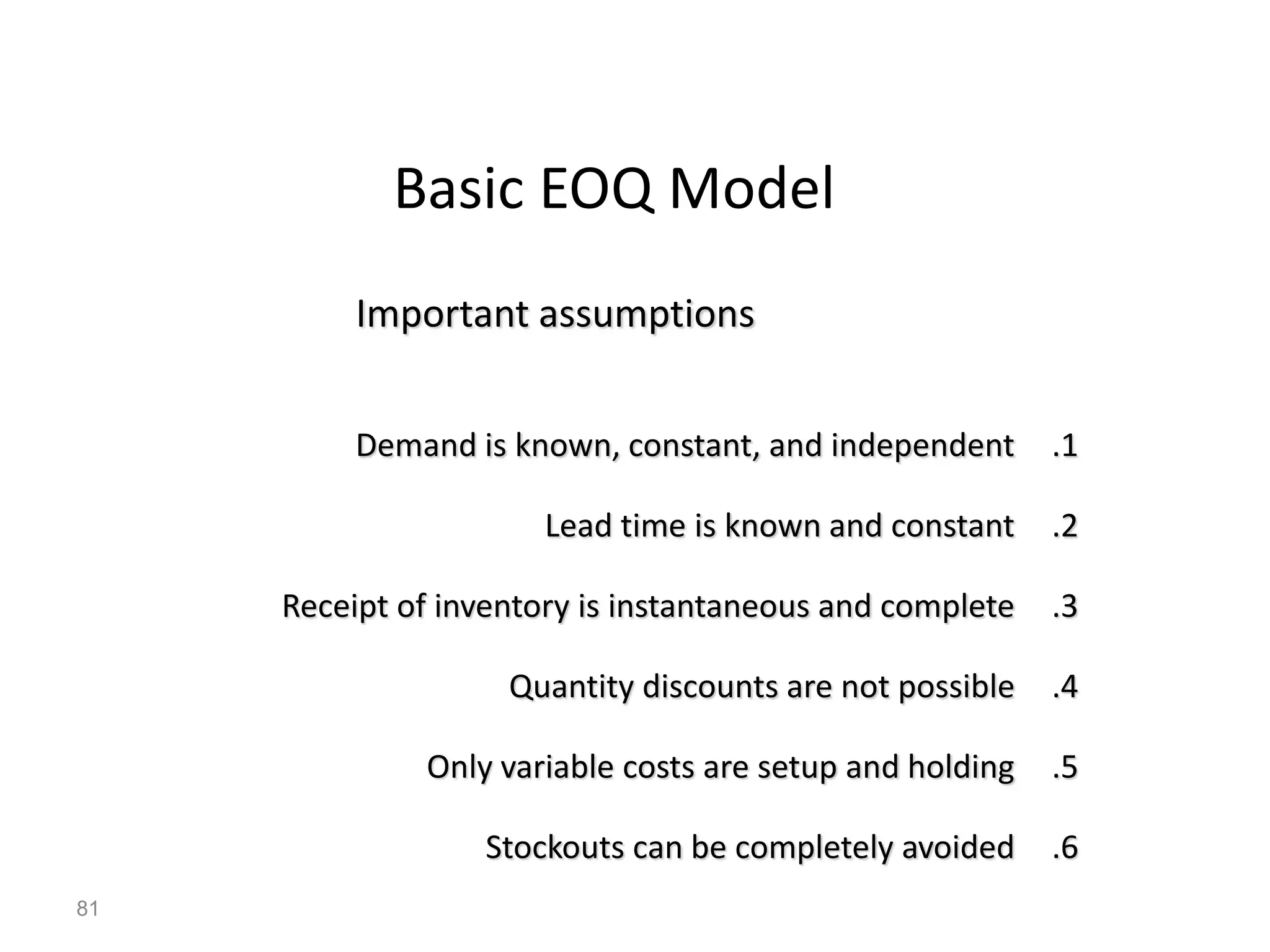
Basic EOQ Model
.1
Demandis known, constant, and independent
.2
Lead time is known and constant
.3
Receipt of inventory is instantaneous and complete
.4
Quantity discounts are not possible
.5
Only variable costs are setup and holding
.6
Stockouts can be completely avoided
Important assumptions
81
82.
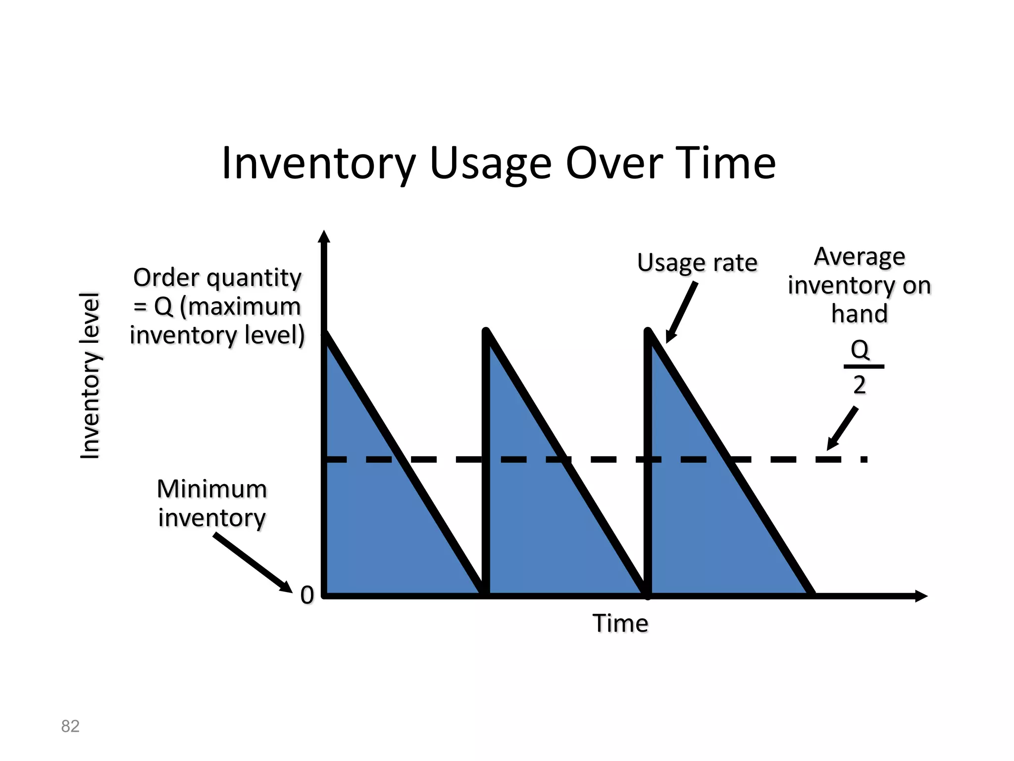
Inventory Usage OverTime
Order quantity
= Q (maximum
inventory level)
Usage rate Average
inventory on
hand
Q
2
Minimum
inventory
Inventory
level
Time
0
82
83.
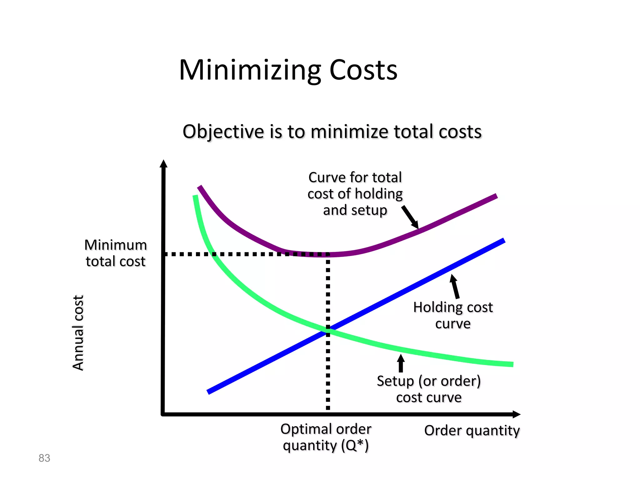
Minimizing Costs
Objective isto minimize total costs
Annual
cost
Order quantity
Curve for total
cost of holding
and setup
Holding cost
curve
Setup (or order)
cost curve
Minimum
total cost
Optimal order
quantity (Q*)
83
84.
The EOQ Model
Q
=Number of pieces per order
Q*
= Optimal number of pieces per order (EOQ)
D
= Annual demand in units for the inventory item
S
= Setup or ordering cost for each order
H
= Holding or carrying cost per unit per year
Annual setup cost =
(Number of orders placed per year)
x (Setup or order cost per order)
Annual demand
Number of units in each order
Setup or order cost
per order
=
Annual setup cost = S
D
Q
= (S)
D
Q
84
85.
= (Holding costper unit per year)
Order quantity
2
The EOQ Model
Q
= Number of pieces per order
Q*
= Optimal number of pieces per order (EOQ)
D
= Annual demand in units for the inventory item
S
= Setup or ordering cost for each order
H
= Holding or carrying cost per unit per year
Annual holding cost =
(Average inventory level)
x (Holding cost per unit per year)
= (H)
Q
2
Annual setup cost = S
D
Q
Annual holding cost = H
Q
2
85
86.
The EOQ Model
Q
=Number of pieces per order
Q*
= Optimal number of pieces per order (EOQ)
D
= Annual demand in units for the inventory item
S
= Setup or ordering cost for each order
H
= Holding or carrying cost per unit per year
Optimal order quantity is found when annual setup cost equals
annual holding cost
D
Q
S = H
Q
2
Solving for Q*
2DS = Q2H
Q2 = 2DS/H
Q* = 2DS/H
Annual setup cost = S
D
Q
Annual holding cost = H
Q
2
86
87.
An EOQ Example
Determineoptimal number of needles to order
D = 1,000 units
S = $10 per order
H = $.50 per unit per year
Q* =
2DS
H
Q* =
2(1,000)(10)
0.50
= 40,000 = 200 units
87
88.
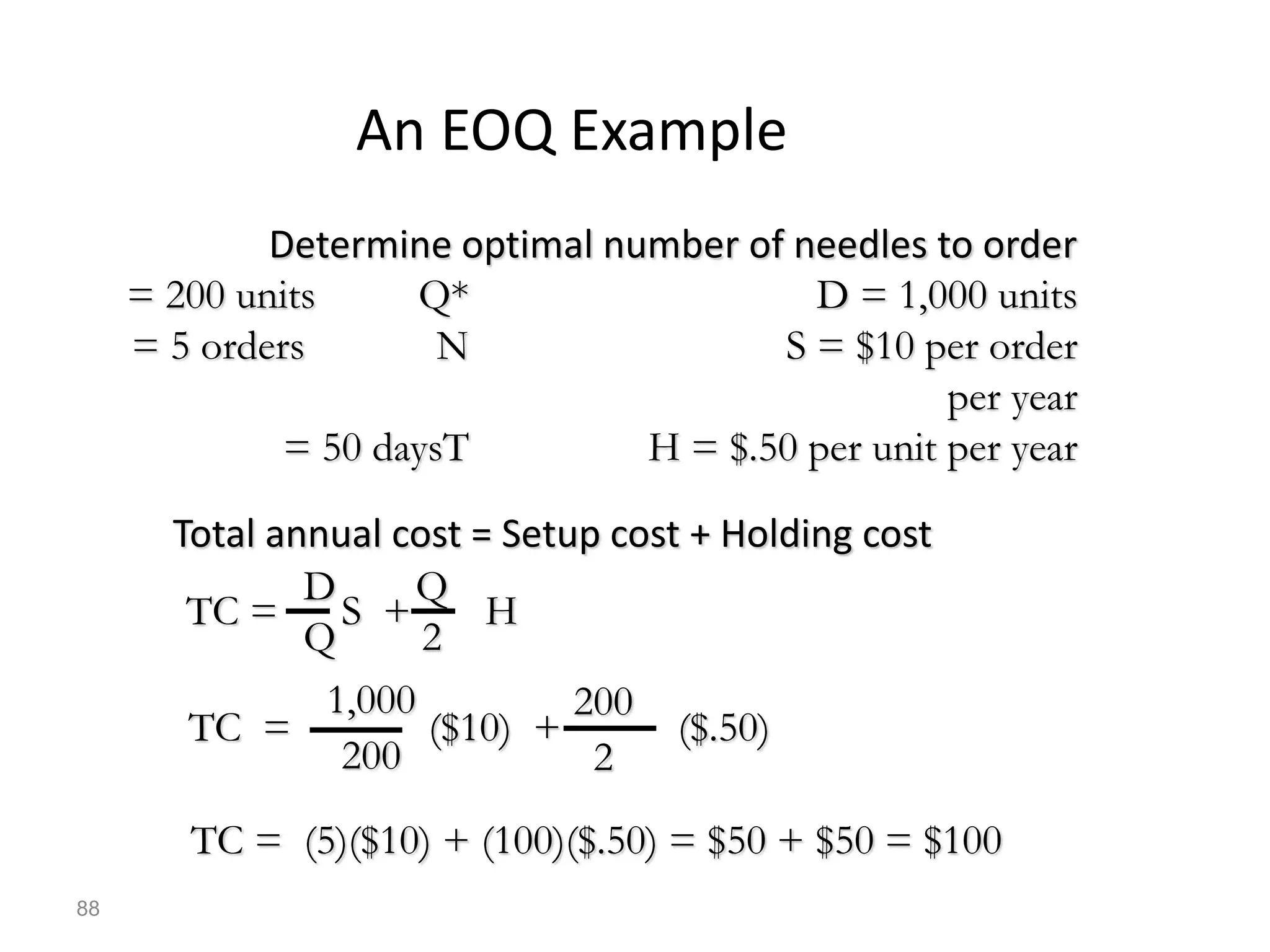
An EOQ Example
Determineoptimal number of needles to order
D = 1,000 units
Q*
= 200 units
S = $10 per order
N
= 5 orders
per year
H = $.50 per unit per year
T
= 50 days
Total annual cost = Setup cost + Holding cost
TC = S + H
D
Q
Q
2
TC = ($10) + ($.50)
1,000
200
200
2
TC = (5)($10) + (100)($.50) = $50 + $50 = $100
88
89.
Reorder Points
EOQ answersthe “how much” question
The reorder point (ROP) tells when to order
ROP =
Lead time for a new
order in days
Demand per
day
= d x L
d = D
Number of working days in a year
89
Reorder Point Example
Demand= 8,000 iPods per year
250 working day year
Lead time for orders is 3 working days
ROP = d x L
d =
D
Number of working days in a year
= 8,000/250 = 32 units
= 32 units per day x 3 days = 96 units
91
Lot-for-Lot Example
1 23 4 5 6 7 8 9 10
Gross
requirements
35 30 40 0 10 40 30 0 30 55
Scheduled
receipts
Projected on
hand
35 35 0 0 0 0 0 0 0 0 0
Net
requirements
0 30 40 0 10 40 30 0 30 55
Planned order
receipts
30 40 10 40 30 30 55
Planned order
releases
30 40 10 40 30 30 55
Holding cost = $1/week; Setup cost = $100; Lead time = 1 week
No on-hand inventory is carried through the system
Total holding cost = $0
There are seven setups for this item in this plan
Total setup cost = 7 x $100 = $700
94.
EOQ Lot SizeExample
1 2 3 4 5 6 7 8 9 10
Gross
requirements
35 30 40 0 10 40 30 0 30 55
Scheduled
receipts
Projected on
hand
35 35 0 43 3 3 66 26 69 69 39
Net
requirements
0 30 0 0 7 0 4 0 0 16
Planned order
receipts
73 73 73 73
Planned order
releases
73 73 73 73
Holding cost = $1/week; Setup cost = $100; Lead time = 1 week
Average weekly gross requirements = 27; EOQ = 73 units
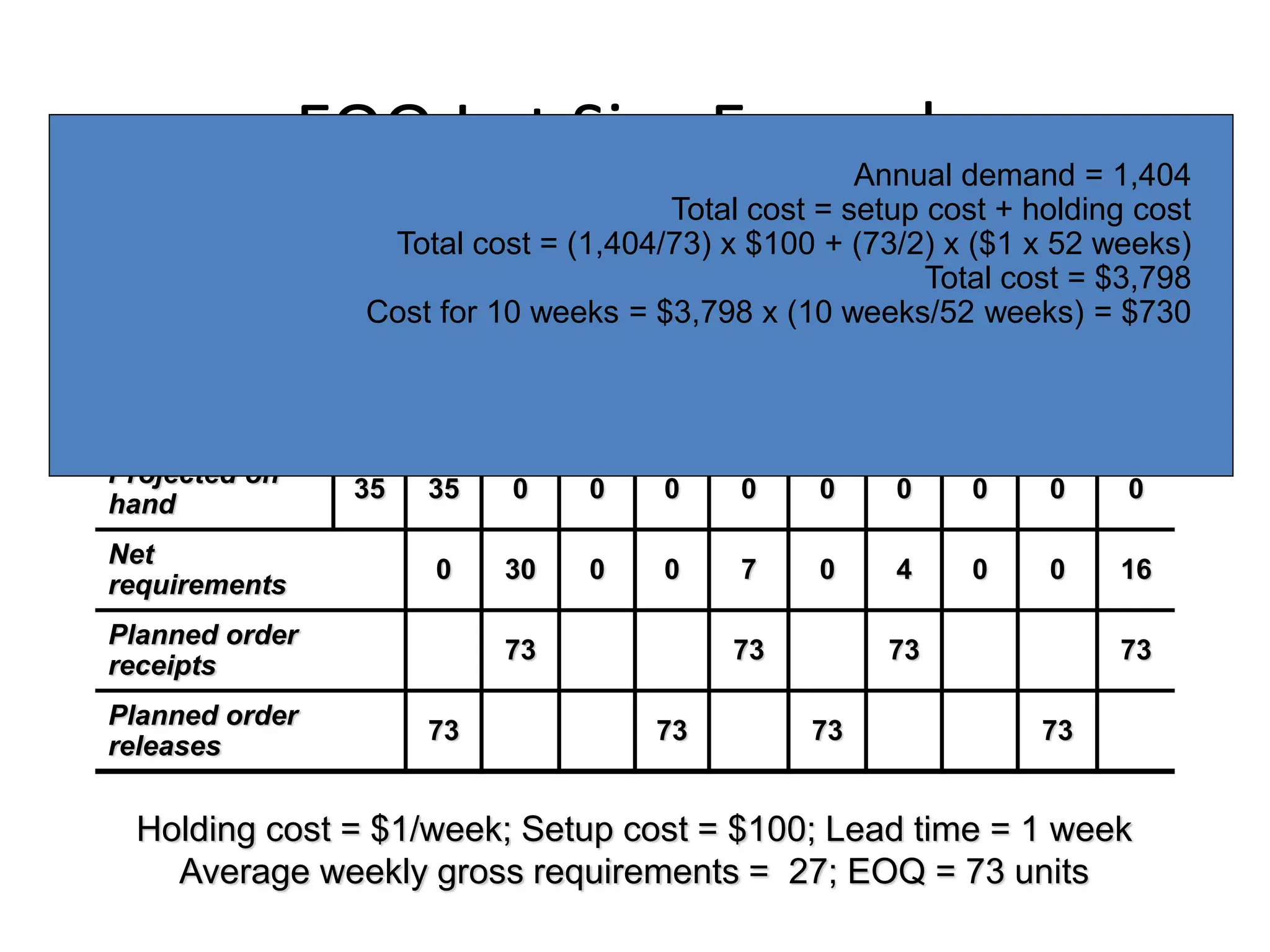
95.
EOQ Lot SizeExample
1 2 3 4 5 6 7 8 9 10
Gross
requirements
35 30 40 0 10 40 30 0 30 55
Scheduled
receipts
Projected on
hand
35 35 0 0 0 0 0 0 0 0 0
Net
requirements
0 30 0 0 7 0 4 0 0 16
Planned order
receipts
73 73 73 73
Planned order
releases
73 73 73 73
Holding cost = $1/week; Setup cost = $100; Lead time = 1 week
Average weekly gross requirements = 27; EOQ = 73 units
Annual demand = 1,404
Total cost = setup cost + holding cost
Total cost = (1,404/73) x $100 + (73/2) x ($1 x 52 weeks)
Total cost = $3,798
Cost for 10 weeks = $3,798 x (10 weeks/52 weeks) = $730
96.
PPB Example
1 23 4 5 6 7 8 9 10
Gross
requirements
35 30 40 0 10 40 30 0 30 55
Scheduled
receipts
Projected on
hand
35
Net
requirements
Planned order
receipts
Planned order
releases
Holding cost = $1/week; Setup cost = $100; Lead time = 1 week
EPP = 100 units
97.
PPB Example
1 23 4 5 6 7 8 9 10
Gross
requirements
35 30 40 0 10 40 30 0 30 55
Scheduled
receipts
Projected on
hand
35
Net
requirements
Planned order
receipts
Planned order
releases
Holding cost = $1/week; Setup cost = $100;
EPP = 100 units
2
30
0
2, 3
70
40 = 40 x 1
2, 3, 4
70
40
2, 3, 4, 5
80
70 = 40 x 1 + 10 x 3
100
70
170
2, 3, 4, 5, 6
120
230 = 40 x 1 + 10 x 3
+ 40 x 4
+ =
Combine periods 2 - 5 as this results in the Part Period
closest to the EPP
Combine periods 6 - 9 as this results in the Part Period
closest to the EPP
6
40
0
6, 7
70
30 = 30 x 1
6, 7, 8
70
30 = 30 x 1 + 0 x 2
6, 7, 8, 9
100
120 = 30 x 1 + 30 x 3
100
120
220 + =
10
55
0
100
0
100
Total cost
300
190
490
+ =
+ =
Trial Lot Size
Periods
(cumulative net
Costs
Combined
requirements)
Part Periods
Setup
Holding
Total
98.
PPB Example
1 23 4 5 6 7 8 9 10
Gross
requirements
35 30 40 0 10 40 30 0 30 55
Scheduled
receipts
Projected on
hand
35 35 0 50 10 10 0 60 30 30 0
Net
requirements
0 30 0 0 0 40 0 0 0 55
Planned order
receipts
80 100 55
Planned order
releases
80 100 55
Holding cost = $1/week; Setup cost = $100; Lead time = 1 week
EPP = 100 units
Lot-Sizing Summary
Intheory, lot sizes should be recomputed
whenever there is a lot size or order quantity
change
In practice, this results in system
nervousness and instability
Lot-for-lot should
be used when
low-cost JIT can
be achieved
101.
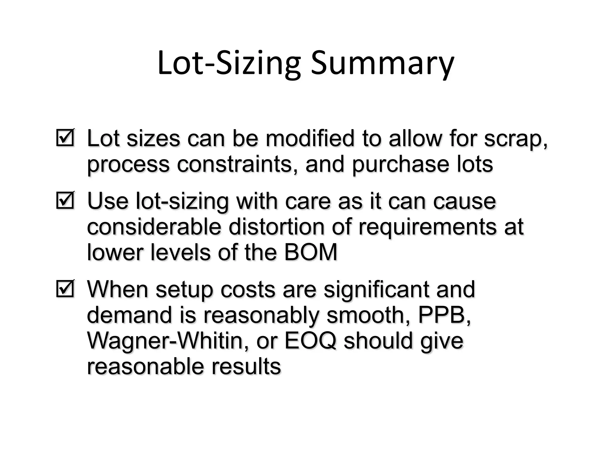
Lot-Sizing Summary
Lotsizes can be modified to allow for scrap,
process constraints, and purchase lots
Use lot-sizing with care as it can cause
considerable distortion of requirements at
lower levels of the BOM
When setup costs are significant and
demand is reasonably smooth, PPB,
Wagner-Whitin, or EOQ should give
reasonable results
102.
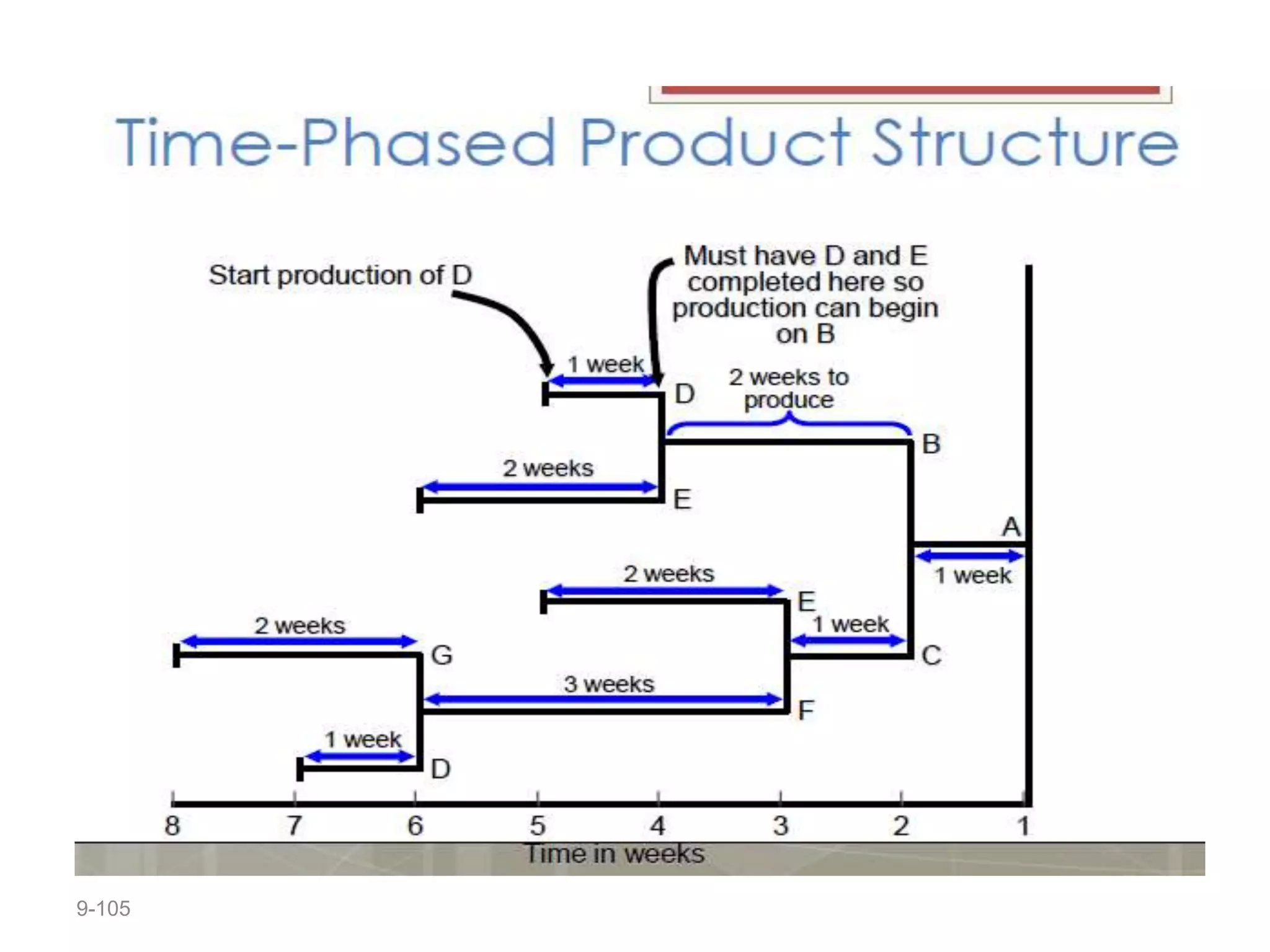
Material Requirements Plan
•
Theplanning horizon is at least as long as the
combined purchase and manufacturing lead
times.
•
As with the master production schedule, it
usually extends from 3 to 18 months.
102