Market
• It isa setting where buyers and sellers to trade goods or services with each
other.
• It can be a real physical place • Or a non-physical market like ebay
or Amazon
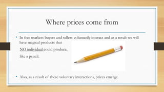
Where prices comefrom
• In free markets buyers and sellers voluntarily interact and as a result we will
have magical products that
NO individual could produce,
like a pencil.
• Also, as a result of these voluntary interactions, prices emerge.
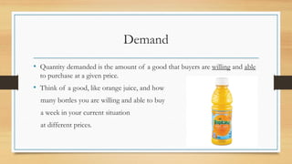
Demand
• Quantity demandedis the amount of a good that buyers are willing and able
to purchase at a given price.
• Think of a good, like orange juice, and how
many bottles you are willing and able to buy
a week in your current situation
at different prices.
7.
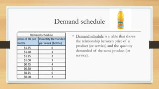
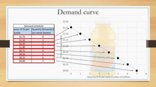
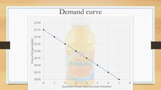
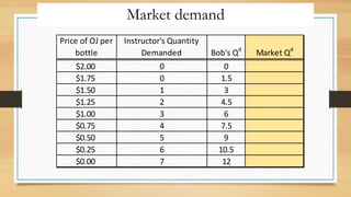
Demand schedule
• Demandschedule is a table that shows
the relationship between price of a
product (or service) and the quantity
demanded of the same product (or
service).
price of OJ per
bottle
Quantity Demanded
per week (bottle)
$1.75 0
$1.50 1
$1.25 2
$1.00 3
$0.75 4
$0.50 5
$0.25 6
$0.00 7
Demand schedule
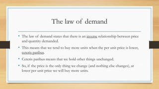
The law ofdemand
• The law of demand states that there is an inverse relationship between price
and quantity demanded.
• This means that we tend to buy more units when the per unit price is lower,
ceteris paribus.
• Ceteris paribus means that we hold other things unchanged.
• So, if the price is the only thing we change (and nothing else changes), at
lower per unit price we will buy more units.
12.
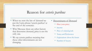
Reason for ceterisparibus
• When we state the law of demand we
put the Latin phrase ‘ceteris paribus’ at
the end of the sentence.
• Why? Because there are other factors
that determine demand, price is not the
only one.
• We say ceteris paribus meaning that
these other determinants are not
changing.
• Determinants of Demand
• Price (own price)
• Income
• Price of related goods
• Tastes and Preferences
• Expectations about the future
• Number of buyers
13.
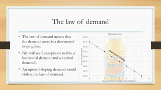
The law ofdemand
• The law of demand means that
the demand curve is a downward-
sloping line.
• (We will see 2 exceptions to this, a
horizontal demand and a vertical
demand.)
• An upward-sloping demand would
violate the law of demand.
14.
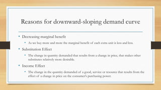
Reasons for downward-slopingdemand curve
• Decreasing marginal benefit
• As we buy more and more the marginal benefit of each extra unit is less and less.
• Substitution Effect
• The change in quantity demanded that results from a change in price, that makes other
substitutes relatively more desirable.
• Income Effect
• The change in the quantity demanded of a good, service or resource that results from the
effect of a change in price on the consumer’s purchasing power.
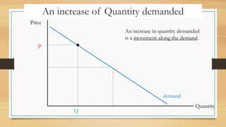
An increase ofQuantity demanded
Price
Quantity
P
Q
An increase in quantity demanded
is a movement along the demand.
demand
22.
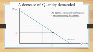
A decrease ofQuantity demanded
Price
Quantity
P
Q
An decrease in quantity demanded is
a movement along the demand.
demand
23.
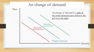
An change ofdemand
Price
Quantity
An change of demand is a shift of
the entire demand curve either to the
left or to the right.
Original demand
increase
decrease
24.
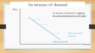
An increase ofdemand
Price
Quantity
An increase in demand is a shift of
the entire demand curve to the right.
Original demand
New, increased
demand
25.
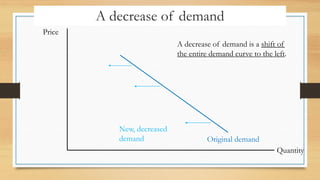
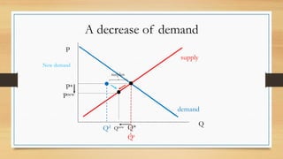
A decrease ofdemand
Price
Quantity
A decrease of demand is a shift of
the entire demand curve to the left.
Original demand
New, decreased
demand
26.
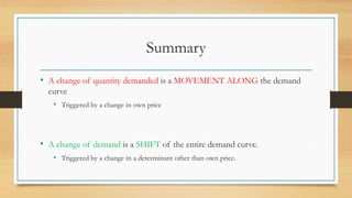
Summary
• A changeof quantity demanded is a MOVEMENT ALONG the demand
curve
• Triggered by a change in own price
• A change of demand is a SHIFT of the entire demand curve.
• Triggered by a change in a determinant other than own price.
Consumer Income
• Weknow that Income is a SHIFT factor – a determinant of demand that if
it changes you need to shift demand.
• How would you need to change demand if incomes increase?
29.
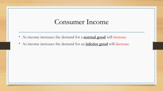
Consumer Income
• Asincome increases the demand for a normal good will increase.
• As income increases the demand for an inferior good will decrease.
30.
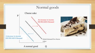
Normal goods
P
Q
Cheese cake
Anincrease in income
INCREASES Demand
A decrease in income
DECREASES Demand
A normal good
Initial demand for cheese
cakes
31.
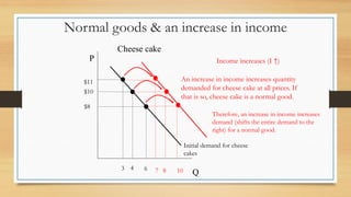
Normal goods &an increase in income
P
Q
Cheese cake
Initial demand for cheese
cakes
$10
4
Income increases (I ↑)
8
$8
6
$11
10
7
3
An increase in income increases quantity
demanded for cheese cake at all prices. If
that is so, cheese cake is a normal good.
Therefore, an increase in income increases
demand (shifts the entire demand to the
right) for a normal good.
32.
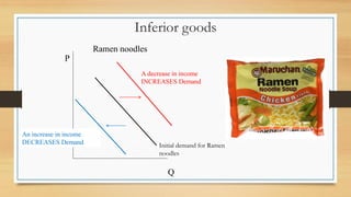
Inferior goods
P
Q
Ramen noodles
Adecrease in income
INCREASES Demand
An increase in income
DECREASES Demand Initial demand for Ramen
noodles
33.
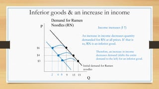
Inferior goods &an increase in income
P
Q
Demand for Ramen
Noodles (RN)
Initial demand for Ramen
noodles
$4
13
Income increases (I ↑)
6
$3
15
$6
8
2 9
An increase in income decreases quantity
demanded for RN at all prices. If that is
so, RN is an inferior good.
Therefore, an increase in income
decreases demand (shifts the entire
demand to the left) for an inferior good.
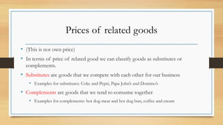
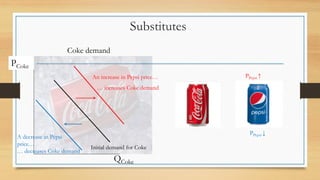
Prices of relatedgoods
• (This is not own price)
• In terms of price of related good we can classify goods as substitutes or
complements.
• Substitutes are goods that we compete with each other for our business
• Examples for substitutes: Coke and Pepsi, Papa John’s and Domino’s
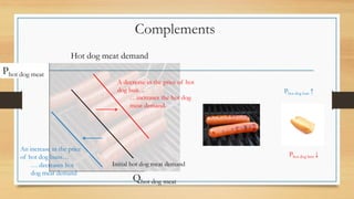
• Complements are goods that we tend to consume together
• Examples for complements: hot dog meat and hot dog bun, coffee and cream
36.
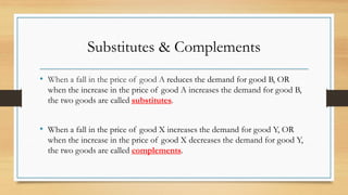
Substitutes & Complements
•When a fall in the price of good A reduces the demand for good B, OR
when the increase in the price of good A increases the demand for good B,
the two goods are called substitutes.
• When a fall in the price of good X increases the demand for good Y, OR
when the increase in the price of good X decreases the demand for good Y,
the two goods are called complements.
Complements
Phot dog meat
Qhotdog meat
Hot dog meat demand
A decrease in the price of hot
dog bun…
An increase in the price
of hot dog buns…
Initial hot dog meat demand
…increases the hot dog
meat demand.
… decreases hot
dog meat demand
Phot dog bun ↑
Phot dog bun ↓
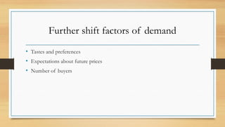
Further shift factorsof demand
• Tastes and preferences
• Expectations about future prices
• Number of buyers
41.
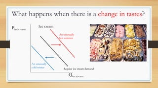
Pice cream
Qice cream
Icecream
An unusually
hot summer
An unusually
cold winter
What happens when there is a change in tastes?
Regular ice cream demand
42.
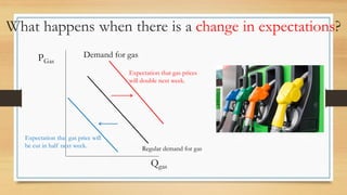
What happens whenthere is a change in expectations?
PGas
Qgas
Demand for gas
Expectation that gas prices
will double next week.
Expectation that gas price will
be cut in half next week. Regular demand for gas
43.
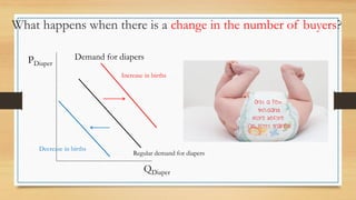
What happens whenthere is a change in the number of buyers?
PDiaper
QDiaper
Demand for diapers
Increase in births
Decrease in births
Regular demand for diapers
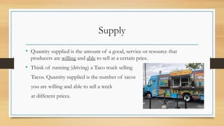
Supply
• Quantity suppliedis the amount of a good, service or resource that
producers are willing and able to sell at a certain price.
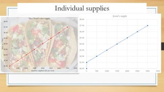
• Think of running (driving) a Taco truck selling
Tacos. Quantity supplied is the number of tacos
you are willing and able to sell a week
at different prices.
46.
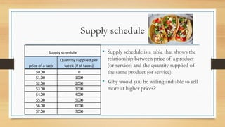
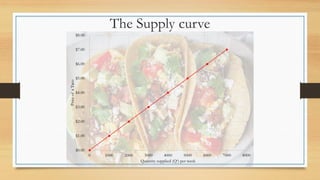
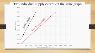
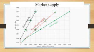
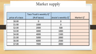
Supply schedule
• Supplyschedule is a table that shows the
relationship between price of a product
(or service) and the quantity supplied of
the same product (or service).
• Why would you be willing and able to sell
more at higher prices?
price of a taco
Quantity supplied per
week (# of tacos)
$0.00 0
$1.00 1000
$2.00 2000
$3.00 3000
$4.00 4000
$5.00 5000
$6.00 6000
$7.00 7000
Supply schedule
47.
$0.00
$1.00
$2.00
$3.00
$4.00
$5.00
$6.00
$7.00
$8.00
0 1000 20003000 4000 5000 6000 7000 8000
Price
of
a
Taco
Quantity supplied (Qs) per week
Supply curve
price of a taco
Quantity supplied per
week (# of tacos)
$0.00 0
$1.00 1000
$2.00 2000
$3.00 3000
$4.00 4000
$5.00 5000
$6.00 6000
$7.00 7000
Supply schedule
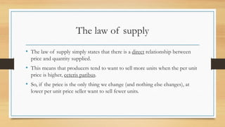
The law ofsupply
• The law of supply simply states that there is a direct relationship between
price and quantity supplied.
• This means that producers tend to want to sell more units when the per unit
price is higher, ceteris paribus.
• So, if the price is the only thing we change (and nothing else changes), at
lower per unit price seller want to sell fewer units.
51.
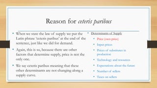
Reason for ceterisparibus
• When we state the law of supply we put the
Latin phrase ‘ceteris paribus’ at the end of the
sentence, just like we did for demand.
• Again, this is so, because there are other
factors that determine supply, price is not the
only one.
• We say ceteris paribus meaning that these
other determinants are not changing along a
supply curve.
• Determinants of Supply
• Price (own price)
• Input prices
• Prices of substitutes in
production
• Technology and resources
• Expectations about the future
• Number of sellers
• Taxes on sellers
52.
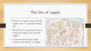
The law ofsupply
• The law of supply means that the
supply curve is a upward-sloping
line.
• (We will see 2 exceptions to this, a
horizontal supply and a vertical
supply.)
• An downward-sloping supply
would violate the law of supply.
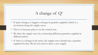
A change ofQs
• If price changes, it triggers a change in quantity supplied, which is a
movement along the supply curve.
• This is so because price is on the vertical axis.
• We drew the supply curve by connecting different quantities supplied at
different prices.
• If there is a change in the price, the supply curve already has a quantity
supplied for that. We do not need to draw a new supply.
60.
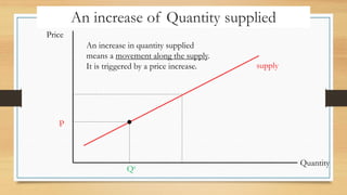
An increase ofQuantity supplied
Price
Quantity
P
Qs
An increase in quantity supplied
means a movement along the supply.
It is triggered by a price increase. supply
61.
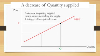
A decrease ofQuantity supplied
Price
Quantity
P
Qs
A decrease in quantity supplied
means a movement along the supply.
It is triggered by a price decrease. supply
62.
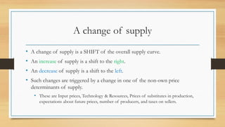
A change ofsupply
• A change of supply is a SHIFT of the overall supply curve.
• An increase of supply is a shift to the right.
• An decrease of supply is a shift to the left.
• Such changes are triggered by a change in one of the non-own price
determinants of supply.
• These are Input prices, Technology & Resources, Prices of substitutes in production,
expectations about future prices, number of producers, and taxes on sellers.
63.
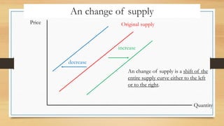
An change ofsupply
Price
Quantity
An change of supply is a shift of the
entire supply curve either to the left
or to the right.
Original supply
increase
decrease
64.
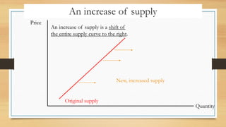
An increase ofsupply
Price
Quantity
An increase of supply is a shift of
the entire supply curve to the right.
Original supply
New, increased supply
65.
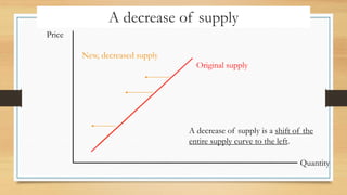
A decrease ofsupply
Price
Quantity
A decrease of supply is a shift of the
entire supply curve to the left.
Original supply
New, decreased supply
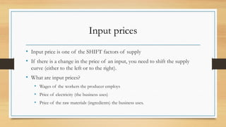
Input prices
• Inputprice is one of the SHIFT factors of supply
• If there is a change in the price of an input, you need to shift the supply
curve (either to the left or to the right).
• What are input prices?
• Wages of the workers the producer employs
• Price of electricity (the business uses)
• Price of the raw materials (ingredients) the business uses.
68.
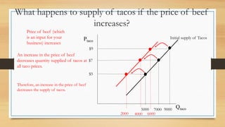
What happens tosupply of tacos if the price of beef
increases?
Ptaco
Qtaco
Initial supply of Tacos
$7
5000
Price of beef (which
is an input for your
business) increases
4000
$5
9000
$9
6000
2000
7000
An increase in the price of beef
decreases quantity supplied of tacos at
all taco prices.
Therefore, an increase in the price of beef
decreases the supply of tacos.
69.
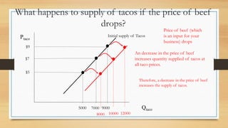
What happens tosupply of tacos if the price of beef
drops?
Ptaco
Qtaco
Initial supply of Tacos
$7
5000
Price of beef (which
is an input for your
business) drops
10000
$5
9000
$9
12000
8000
7000
An decrease in the price of beef
increases quantity supplied of tacos at
all taco prices.
Therefore, a decrease in the price of beef
increases the supply of tacos.
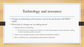
Technology and resources
•Changes in technology and resources used in the production will SHIFT
supply
• What kind of changes are we talking about?
• Improvement in technology
• The invention of computers, the internet, etc. had a huge impact on many industries, making
it easier to produce goods or services
• One of your workers invents a more efficient production method
• But it could also be a natural disaster that destroys factories
72.
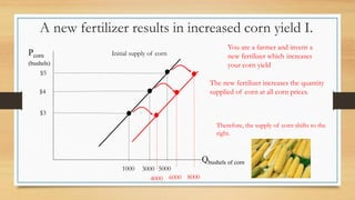
Pcorn
(bushels)
Qbushels of corn
Initialsupply of corn
$4
1000
You are a farmer and invent a
new fertilizer which increases
your corn yield
6000
$3
5000
$5
8000
4000
3000
The new fertilizer increases the quantity
supplied of corn at all corn prices.
Therefore, the supply of corn shifts to the
right.
A new fertilizer results in increased corn yield I.
73.
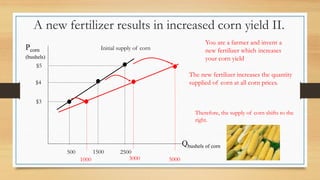
Pcorn
(bushels)
Qbushels of corn
Initialsupply of corn
$4
500
You are a farmer and invent a
new fertilizer which increases
your corn yield
3000
$3
2500
$5
5000
1000
1500
The new fertilizer increases the quantity
supplied of corn at all corn prices.
Therefore, the supply of corn shifts to the
right.
A new fertilizer results in increased corn yield II.
74.
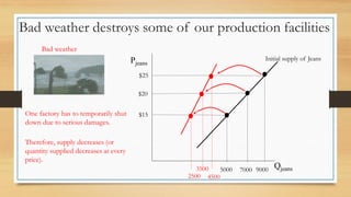
Bad weather destroyssome of our production facilities
Pjeans
Qjeans
Initial supply of Jeans
$20
5000
Bad weather
3500
$15
9000
$25
4500
2500
7000
One factory has to temporarily shut
down due to serious damages.
Therefore, supply decreases (or
quantity supplied decreases at every
price).
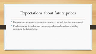
Expectations about futureprices
• Expectations are quite important to producers as well (not just consumers)
• Producers may slow down or ramp up production based on what they
anticipate the future brings
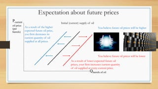
77.
Pcurrent
oil price
(per
barrels)
Qbarrels ofoil
Initial (current) supply of oil
As a result of lower expected future oil
prices, your firm increases current quantity
of oil supplied at every current price.
Expectation about future prices
You believe future oil prices will be higher
You believe future oil prices will be lower
As a result of the higher
expected future oil price,
you firm decreases its
current quantity of oil
supplied at all prices.
78.
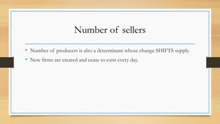
Number of sellers
•Number of producers is also a determinant whose change SHIFTS supply.
• New firms are created and cease to exist every day.
79.
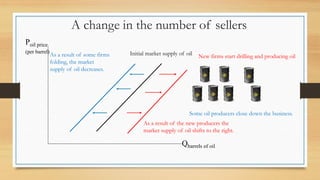
Poil price
(per barrel)
Qbarrelsof oil
Initial market supply of oil
As a result of the new producers the
market supply of oil shifts to the right.
A change in the number of sellers
New firms start drilling and producing oil
Some oil producers close down the business.
As a result of some firms
folding, the market
supply of oil decreases.
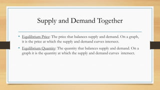
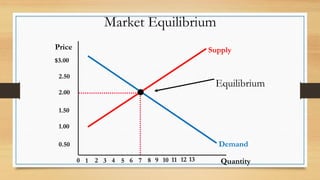
Supply and DemandTogether
• Equilibrium Price: The price that balances supply and demand. On a graph,
it is the price at which the supply and demand curves intersect.
• Equilibrium Quantity: The quantity that balances supply and demand. On a
graph it is the quantity at which the supply and demand curves intersect.
82.
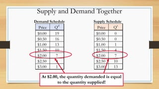
Supply and DemandTogether
Demand Schedule Supply Schedule
At $2.00, the quantity demanded is equal
to the quantity supplied!
Price Qd
$0.00 19
$0.50 16
$1.00 13
$1.50 10
$2.00 7
$2.50 4
$3.00 1
Price Qs
$0.00 0
$0.50 0
$1.00 1
$1.50 4
$2.00 7
$2.50 10
$3.00 13
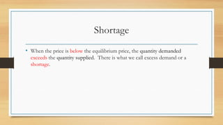
Shortage
• When theprice is below the equilibrium price, the quantity demanded
exceeds the quantity supplied. There is what we call excess demand or a
shortage.
86.
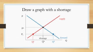
Draw a graphwith a shortage
P
Q
P*
P1
Q*
Qs Qd
shortage demand
supply
87.
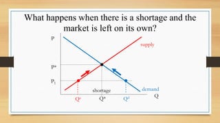
What happens whenthere is a shortage and the
market is left on its own?
P
Q
P*
P1
Q*
Qs Qd
shortage demand
supply
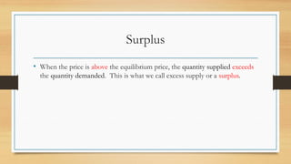
Surplus
• When theprice is above the equilibrium price, the quantity supplied exceeds
the quantity demanded. This is what we call excess supply or a surplus.
90.
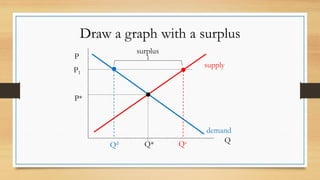
Draw a graphwith a surplus
P
Q
P*
P1
Q* Qs
Qd
surplus
demand
supply
91.
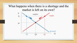
What happens whenthere is a shortage and the
market is left on its own?
P
Q
P*
P1
Q* Qs
Qd
surplus
demand
supply
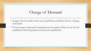
Change of Demand
•Imagine that the market starts out in equilibrium and then, there is a change
in demand.
• If that change in demand is instantaneous, the market will be out of the old
equilibrium and will gravitate toward a new equilibrium.
94.
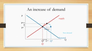
An increase ofdemand
P
Q
P*
Q*
Qs
Qd
demand
supply
Pnew
Qnew
shortage
New demand
A decrease ofdemand
P
Q
P*
Q*
Qs
Qd
demand
supply
Pnew
Qnew
surplus
New demand
97.
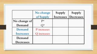
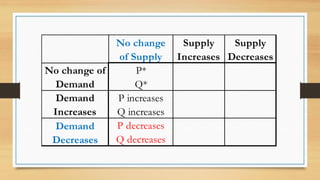
P*
Q*
P increases
Q increases
Pdecreases
Q decreases
Demand
Decreases
No change of
Demand
No change
of Supply
Supply
Increases
Supply
Decreases
Demand
Increases
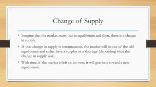
Change of Supply
•Imagine that the market starts out in equilibrium and then, there is a change
in supply.
• If that change in supply is instantaneous, the market will be out of the old
equilibrium and either have a surplus or a shortage (depending what the
change in supply was).
• With time, if the market is left on its own, it will gravitate toward a new
equilibrium.
100.
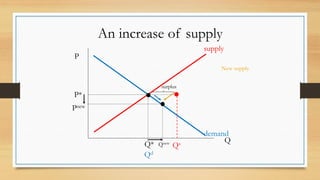
An increase ofsupply
P
Q
P*
Q* Qs
Qd
demand
supply
Pnew
Qnew
surplus
New supply
101.
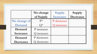
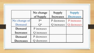
P* P decreases
Q*Q increases
P increases
Q increases
P decreases
Q decreases
Demand
Decreases
No change of
Demand
No change
of Supply
Supply
Increases
Supply
Decreases
Demand
Increases
102.
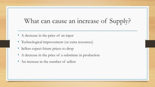
What can causean increase of Supply?
• A decrease in the price of an input
• Technological improvement (or extra resources)
• Sellers expect future prices to drop
• A decrease in the price of a substitute in production
• An increase in the number of sellers
103.
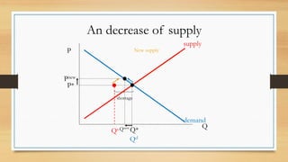
An decrease ofsupply
P
Q
P*
Q*
Qs
Qd
demand
supply
Pnew
Qnew
shortage
New supply
104.
P* P decreasesP increases
Q* Q increases Q decreases
P increases
Q increases
P decreases
Q decreases
Demand
Decreases
No change of
Demand
No change
of Supply
Supply
Increases
Supply
Decreases
Demand
Increases
105.
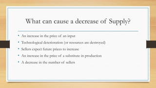
What can causea decrease of Supply?
• An increase in the price of an input
• Technological deterioration (or resources are destroyed)
• Sellers expect future prices to increase
• An increase in the price of a substitute in production
• A decrease in the number of sellers
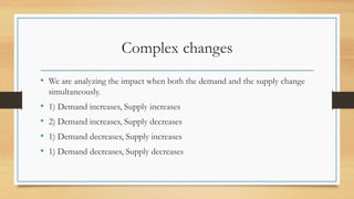
Complex changes
• Weare analyzing the impact when both the demand and the supply change
simultaneously.
• 1) Demand increases, Supply increases
• 2) Demand increases, Supply decreases
• 1) Demand decreases, Supply increases
• 1) Demand decreases, Supply decreases
108.
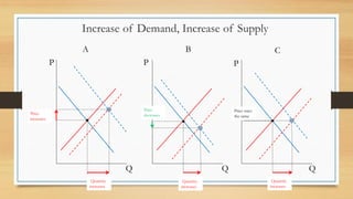
Increase of Demand,Increase of Supply
Q
P
Q
P
Q
P
A B C
Price
increases
Quantity
increases
Quantity
increases
Quantity
increases
Price
decreases
Price stays
the same
109.
P* P decreasesP increases
Q* Q increases Q decreases
P increases P uncertain
Q increases Q increases
P decreases
Q decreases
Demand
Decreases
No change of
Demand
No change
of Supply
Supply
Increases
Supply
Decreases
Demand
Increases
110.
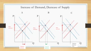
Increase of Demand,Decrease of Supply
Q
P
Q
P
Q
P
A B C
Price
increases
Quantity
increases
Quantity
decreases
Quantity
stays the
same
Price
increases
Price
increases
111.
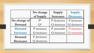
P* P decreasesP increases
Q* Q increases Q decreases
P increases P uncertain P increases
Q increases Q increases Q uncertain
P decreases
Q decreases
Demand
Decreases
No change of
Demand
No change
of Supply
Supply
Increases
Supply
Decreases
Demand
Increases
112.
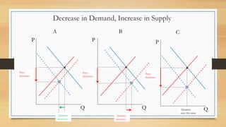
Decrease in Demand,Increase in Supply
Q
P
Q
P
Q
P
A B C
Price
decreases
Quantity
decreases
Quantity
increases
Quantity
stays the same
Price
decreases
Price
decreases
113.
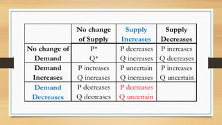
P* P decreasesP increases
Q* Q increases Q decreases
P increases P uncertain P increases
Q increases Q increases Q uncertain
P decreases P decreases
Q decreases Q uncertain
Demand
Decreases
No change of
Demand
No change
of Supply
Supply
Increases
Supply
Decreases
Demand
Increases
114.
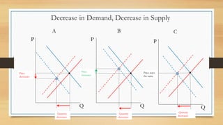
Decrease in Demand,Decrease in Supply
Q
P
Q
P
Q
P
A B C
Price
decreases
Quantity
decreases
Quantity
decreases
Quantity
decreases
Price
increases
Price stays
the same
115.
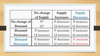
P* P decreasesP increases
Q* Q increases Q decreases
P increases P uncertain P increases
Q increases Q increases Q uncertain
P decreases P decreases P uncertain
Q decreases Q uncertain Q decreases
Demand
Decreases
No change of
Demand
No change
of Supply
Supply
Increases
Supply
Decreases
Demand
Increases
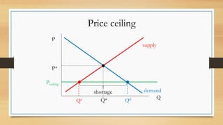
Price ceiling
• Priceceiling is a type of government regulation when the government sets
the maximum allowable price at which goods or services can be exchanged.
• If the price ceiling is set below the equilibrium price, it results in a shortage.
• The market will NOT be able to reach equilibrium because of the
government intervention – in the form of the price ceiling.
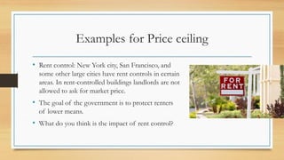
Examples for Priceceiling
• Rent control: New York city, San Francisco, and
some other large cities have rent controls in certain
areas. In rent-controlled buildings landlords are not
allowed to ask for market price.
• The goal of the government is to protect renters
of lower means.
• What do you think is the impact of rent control?
120.
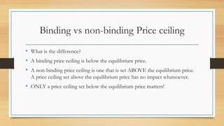
Binding vs non-bindingPrice ceiling
• What is the difference?
• A binding price ceiling is below the equilibrium price.
• A non-binding price ceiling is one that is set ABOVE the equilibrium price.
A price ceiling set above the equilibrium price has no impact whatsoever.
• ONLY a price ceiling set below the equilibrium price matters!
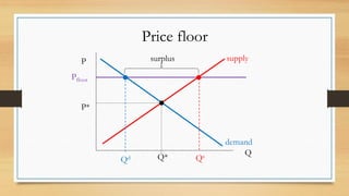
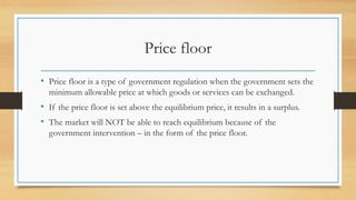
Price floor
• Pricefloor is a type of government regulation when the government sets the
minimum allowable price at which goods or services can be exchanged.
• If the price floor is set above the equilibrium price, it results in a surplus.
• The market will NOT be able to reach equilibrium because of the
government intervention – in the form of the price floor.
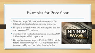
Examples for Pricefloor
• Minimum wage: We have minimum wage at the
federal, State level and even in some cities, etc.
• If a job is covered by the law, it is illegal to pay less
than a certain $$$ per hour.
• The state with the highest minimum wage (in 2020)
is Washington with $13 per hour.
• Georgia’s minimum wage is $5.15 (in 2020), but the
federal minimum wage of $7.25 supersedes it for
jobs covered by the Fair Labor Standards Act.
125.
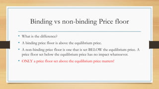
Binding vs non-bindingPrice floor
• What is the difference?
• A binding price floor is above the equilibrium price.
• A non-binding price floor is one that is set BELOW the equilibrium price. A
price floor set below the equilibrium price has no impact whatsoever.
• ONLY a price floor set above the equilibrium price matters!
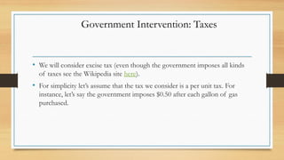
• We willconsider excise tax (even though the government imposes all kinds
of taxes see the Wikipedia site here).
• For simplicity let’s assume that the tax we consider is a per unit tax. For
instance, let’s say the government imposes $0.50 after each gallon of gas
purchased.
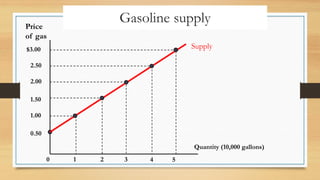
Government Intervention: Taxes
$3.00
2.50
2.00
1.50
1.00
0.50
2
1 3 45
Price
of gas
Quantity (10,000 gallons)
0
Gasoline supply after tax
Supply
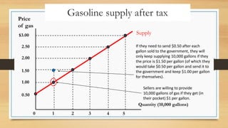
Sellers are willing to provide
10,000 gallons of gas if they get (in
their pocket) $1 per gallon.
If they need to send $0.50 after each
gallon sold to the government, they will
only keep supplying 10,000 gallons if they
the price is $1.50 per gallon (of which they
would take $0.50 per gallon and send it to
the government and keep $1.00 per gallon
for themselves).
130.
$3.00
2.50
2.00
1.50
1.00
0.50
2
1 3 45
Price
of gas
Quantity (10,000 gallons)
0
Gasoline supply after tax
Supply
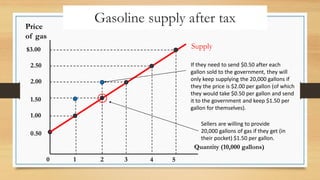
Sellers are willing to provide
20,000 gallons of gas if they get (in
their pocket) $1.50 per gallon.
If they need to send $0.50 after each
gallon sold to the government, they will
only keep supplying the 20,000 gallons if
they the price is $2.00 per gallon (of which
they would take $0.50 per gallon and send
it to the government and keep $1.50 per
gallon for themselves).
131.
$3.00
2.50
2.00
1.50
1.00
0.50
2
1 3 45
Price
of gas
Quantity (10,000 gallons)
0
Gasoline supply after tax
Supply
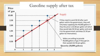
Sellers are willing to provide
30,000 gallons of gas if they get (in
their pocket) $2.00 per gallon.
If they need to send $0.50 after each
gallon sold to the government, they will
only keep supplying the 30,000 gallons if
they the price is $2.50 per gallon (of which
they would take $0.50 per gallon and send
it to the government and keep $2.00 per
gallon for themselves).
132.
$3.00
2.50
2.00
1.50
1.00
0.50
2
1 3 45
Price
of gas
Quantity (10,000 gallons)
0
Gasoline supply after tax
Supply
Sellers are willing to provide
40,000 gallons of gas if they get (in
their pocket) $2.50 per gallon.
If they need to send $0.50 after each
gallon sold to the government, they will
only keep supplying the 40,000 gallons if
they the price is $3.00 per gallon (of which
they would take $0.50 per gallon and send
it to the government and keep $2.50 per
gallon for themselves).
133.
$3.00
2.50
2.00
1.50
1.00
0.50
2
1 3 45
Price
of gas
Quantity (10,000 gallons)
0
Gasoline supply after tax
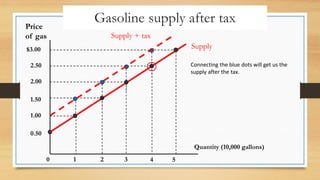
Supply
Supply + tax
Connecting the blue dots will get us the
supply after the tax.
134.
$3.00
2.50
2.00
1.50
1.00
0.50
2
1 3 45
Price
of gas
Quantity (10,000 gallons)
0
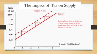
The Impact of Tax on Supply
Supply
Supply + tax
$0.50
$0.50
$0.50
Essentially, we observe the impact
of a tax on the supply as if the
supply were SHIFTED UP by the
amount of the tax.
135.
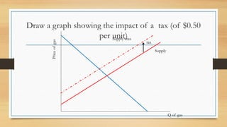
Draw a graphshowing the impact of a tax (of $0.50
per unit)
Price
of
gas
Q of gas
tax
Supply
Supply+tax
136.
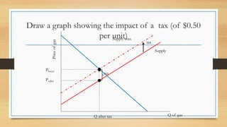
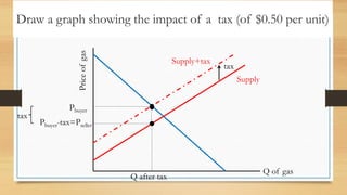
Draw a graphshowing the impact of a tax (of $0.50
per unit)
Price
of
gas
Q of gas
tax
Supply
Supply+tax
Pbuyer
Pseller
tax
Q after tax
137.
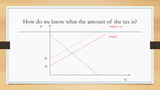
How do weknow what the amount of the tax is?
Supply
Supply+tax
25
18
P
Q
138.
Price floor
• Pricefloor is a type of government regulation when the government sets the
minimum allowable price at which goods or services can be exchanged.
• If the price floor is set above the equilibrium price, it results in a surplus.
• The market will NOT be able to reach equilibrium because of the
government intervention – in the form of the price floor.
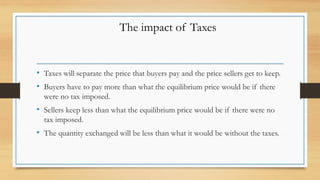
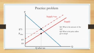
• Taxes willseparate the price that buyers pay and the price sellers get to keep.
• Buyers have to pay more than what the equilibrium price would be if there
were no tax imposed.
• Sellers keep less than what the equilibrium price would be if there were no
tax imposed.
• The quantity exchanged will be less than what it would be without the taxes.
The impact of Taxes
141.
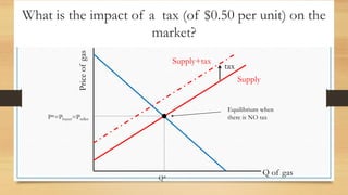
What is theimpact of a tax (of $0.50 per unit) on the
market?
Price
of
gas
Q of gas
tax
Supply
Supply+tax
Equilibrium when
there is NO tax
P*=Pbuyer=Pseller
Q*
142.
Draw a graphshowing the impact of a tax (of $0.50 per unit)
Price
of
gas
Q of gas
tax
Supply
Supply+tax
Pbuyer
Pbuyer-tax=Pseller
tax
Q after tax
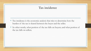
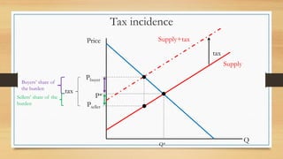
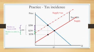
• Tax incidenceis the economic analysis that tries to determine how the
burden of the tax is shared between the buyer and the seller.
• In other words, what portion of the tax falls on buyers; and what portion of
the tax falls on sellers.
Tax incidence