The document covers the design process for timber structures, detailing interconnected stages from concept development to construction specifications. It includes design considerations for various limit states, material properties, load types, and service classes, along with methods for verifying strength using partial factors. The course aims to equip engineers with skills necessary for structural analysis and design of timber materials, referencing multiple Eurocode standards and additional resources.
![1
STRUCTURAL ENGINEERING II: TIMBER DESIGN
INTRODUCTION
The design process included various stages which are interconnected. It starts with the development of a
concept and ends with the detailing of structural parts and the formulation of specifications for construction.
In between, there is the identification of materials and load types, quantification of loads, structural
idealisations and modelling, structural analysis and numerical design.
This course is concerned with the development of skills to complete each of those stages, as a first
approximation to a more comprehensive knowledge and understanding of structural analysis and design.
COURSE CONTENTS
1. BASIS FOR DESIGN PAGE
1.1 ULS GENERAL CONSIDERATION 2
1.2 SLS GENERAL CONSIDERATION 2
1.3 BASIC VARIABLES 2
1.4 LOAD DURATION CASES 2
1.5 SERVICE CLASSES 3
1.6 MATERIAL PROPERTIES 3
1.7 LOAD DURATION AND MOISTURE INFLUECNE ON DEFORMATIONS 3
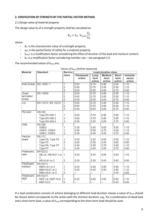
2. VERIFICATION OF STRENGTH BY THE PARTIAL FACTOR METHOD
2.1 DESIGN VALUE OF MATERIAL PROPERTY 6
2.2 MODIFICATION FACTOR FOR SERVICE CLASS 7
3. ULTIMATE LIMIT STATE
3.1 GENERAL 8
3.2 STRENGTH CLASS 9
3.3 DESIGN OF SECTIONS SUBJECT TO STRESS IN ONE DIRECTION 10
3.4 LOAD DURATION AND MOISTURE INFLUENCE ON STRENGTH
4. STABILITY OF MEMBERS
4.1 COLUMNS SUBJECT TO COMPRESSION AND OR BENDING
5. SERVICEABILITY: DEFLECTIONS CHECK
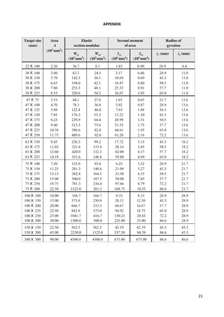
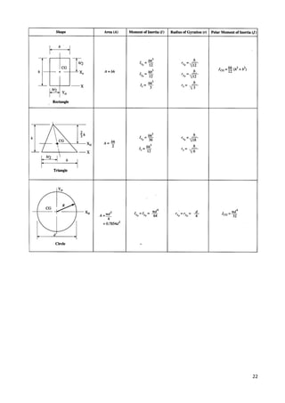
APPENDIX: SECTION PROPERTIES FOR RECTANGULAR SOLID TIMBER
READING LIST
[1] BS EN 1995-1-1: 2004+A2: 2014. Eurocode 4: Design of timber structures. BSI British Standards.
[2] Draycott T and Bullman P, 2009. Structural elements design manual- Working with Eurocodes. Elsevier.
[3] BS EN 338:2016. Structural timber — Strength classes. BSI British Standards.
[4] BS EN 1990: 2000+A1: 2005. Eurocode – basis for Structural design. BSI British Standards.
[5] Porteous J, Ross P, 2013. Designers’ guide to eurocode 5: Design of timber buildings EN 1995-1-1.](https://image.slidesharecdn.com/se-iitimberdesignv4-241117132917-14534bf1/85/Structural-Analysis-Design-Timber-Design-Notes-1-320.jpg)
![1
STRUCTURAL ENGINEERING II: TIMBER DESIGN
INTRODUCTION
The design process included various stages which are interconnected. It starts with the development of a
concept and ends with the detailing of structural parts and the formulation of specifications for construction.
In between, there is the identification of materials and load types, quantification of loads, structural
idealisations and modelling, structural analysis and numerical design.
This course is concerned with the development of skills to complete each of those stages, as a first
approximation to a more comprehensive knowledge and understanding of structural analysis and design.
COURSE CONTENTS
1. BASIS FOR DESIGN PAGE
1.1 ULS GENERAL CONSIDERATION 2
1.2 SLS GENERAL CONSIDERATION 2
1.3 BASIC VARIABLES 2
1.4 LOAD DURATION CASES 2
1.5 SERVICE CLASSES 3
1.6 MATERIAL PROPERTIES 3
1.7 LOAD DURATION AND MOISTURE INFLUECNE ON DEFORMATIONS 3
2. VERIFICATION OF STRENGTH BY THE PARTIAL FACTOR METHOD
2.1 DESIGN VALUE OF MATERIAL PROPERTY 6
2.2 MODIFICATION FACTOR FOR SERVICE CLASS 7
3. ULTIMATE LIMIT STATE
3.1 GENERAL 8
3.2 STRENGTH CLASS 9
3.3 DESIGN OF SECTIONS SUBJECT TO STRESS IN ONE DIRECTION 10
3.4 LOAD DURATION AND MOISTURE INFLUENCE ON STRENGTH
4. STABILITY OF MEMBERS
4.1 COLUMNS SUBJECT TO COMPRESSION AND OR BENDING
5. SERVICEABILITY: DEFLECTIONS CHECK
APPENDIX: SECTION PROPERTIES FOR RECTANGULAR SOLID TIMBER
READING LIST
[1] BS EN 1995-1-1: 2004+A2: 2014. Eurocode 4: Design of timber structures. BSI British Standards.
[2] Draycott T and Bullman P, 2009. Structural elements design manual- Working with Eurocodes. Elsevier.
[3] BS EN 338:2016. Structural timber — Strength classes. BSI British Standards.
[4] BS EN 1990: 2000+A1: 2005. Eurocode – basis for Structural design. BSI British Standards.
[5] Porteous J, Ross P, 2013. Designers’ guide to eurocode 5: Design of timber buildings EN 1995-1-1.](https://image.slidesharecdn.com/se-iitimberdesignv4-241117132917-14534bf1/75/Structural-Analysis-Design-Timber-Design-Notes-1-2048.jpg)
![2
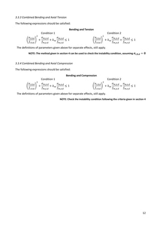
1. BASIS FOR DESIGN
The sections below are made of extracts of Eurocode 5: Design of timber structures and additional teaching
materials added to the reading list.
The design models for the different limit states shall, as appropriate, consider the following:
▪ different material properties (e.g., strength and stiffness).
▪ different time-dependent behaviour of the materials (duration of load, creep).
▪ different climatic conditions (temperature, moisture variations).
▪ different design situations (stages of construction, change of support conditions).
1.1 ULS General considerations
The analysis of structures shall be carried out using the following values for stiffness properties:
▪ for a first order linear elastic analysis of a structure, whose distribution of internal forces is not
affected by the stiffness distribution within the structure (e.g., all members have the same time-
dependent properties), mean values shall be used.
▪ for a first order linear elastic analysis of a structure, whose distribution of internal forces is affected
by the stiffness distribution within the structure (e.g., composite members containing materials
having different time-dependent properties), final mean values adjusted to the load component
causing the largest stress in relation to strength shall be used.
▪ for a second order linear elastic analysis of a structure, design values, not adjusted for duration of
load, shall be used.
1.2 SLS General considerations
The deformation of a structure which results from the effects of actions (such as axial and shear forces,
bending moments and joint slip) and from moisture shall remain within appropriate limits, having regard to
the possibility of damage to surfacing materials, ceilings, floors, partitions and finishes, and to the functional
needs as well as any appearance requirements.
1.3 Basic Variables
The deformation of a structure which results from the effects of actions (such as axial and shear forces,
Actions to be used in design may be obtained from the relevant parts of EN 1991.
Note 1: The relevant parts of EN 1991 for use in design include:
− EN 1991-1-1 Densities, self-weight and imposed loads
− EN 1991-1-3 Snow loads
− EN 1991-1-4 Wind actions
− EN 1991-1-5 Thermal actions
− EN 1991-1-6 Actions during execution
− EN 1991-1-7 Accidental actions
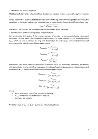
Duration of load and moisture content affect the strength and stiffness properties of timber and wood-based
elements and shall be taken into account in the design for mechanical resistance and serviceability.
1.4 Load-duration classes
The load-duration classes are characterised by the effect of a constant load acting for a certain period of time
in the life of the structure. For a variable action the appropriate class shall be determined on the basis of an
estimate of the typical variation of the load with time.
Actions shall be assigned to one of the load-duration classes given in Table 2.1 in [1] for strength and stiffness
calculations.](https://image.slidesharecdn.com/se-iitimberdesignv4-241117132917-14534bf1/85/Structural-Analysis-Design-Timber-Design-Notes-2-320.jpg)
![3
Load- duration classes (source [1]).
Examples of Load- duration assignment (source [1]).
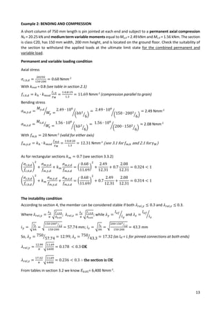
1.5 Service classes
▪ Structures shall be assigned to one of the service classes given below:
NOTE 1: The service class system is mainly aimed at assigning strength values and for calculating deformations under
defined environmental conditions.
NOTE 2: Information on the assignment of structures to service classes given in (2)P, (3)P and (4)P may be given in the
National annex.
▪ Service class 1 is characterised by a moisture content in the materials corresponding to a
temperature of 20°C and the relative humidity of the surrounding air only exceeding 65 % for a
few weeks per year.
NOTE: In service class 1 the average moisture content in most softwoods will not exceed 12 %.
▪ Service class 2 is characterised by a moisture content in the materials corresponding to a
temperature of 20°C and the relative humidity of the surrounding air only exceeding 85 % for a few
weeks per year.
NOTE: In service class 2 the average moisture content in most softwoods will not exceed 20 %.
▪ Service class 3 is characterised by climatic conditions leading to higher moisture contents than in
service class 2.](https://image.slidesharecdn.com/se-iitimberdesignv4-241117132917-14534bf1/85/Structural-Analysis-Design-Timber-Design-Notes-3-320.jpg)
![5
Recommended values of ψ factors for buildings (source [4]).
Recommended values of kdef (source [1])](https://image.slidesharecdn.com/se-iitimberdesignv4-241117132917-14534bf1/85/Structural-Analysis-Design-Timber-Design-Notes-5-320.jpg)
![7
The recommended partial factors for material properties (γM) are,
Recommended partial factors of safety for material properties and resistances (source [1]).
2.2 Modification factors for service class
2.2.1 Solid timber
For rectangular solid timber with a characteristic timber density ρk ≤ 700 kg/m3
the reference depth in
bending or width (maximum cross-sectional dimension) in tension is 150 mm. For depths in bending or widths
in tension of solid timber less than 150 mm, the characteristic strength may be increased by the factor kh,
given by:
𝑘ℎ = 𝑚𝑖𝑛 {
150
ℎ
0.2
1.3
}
where h is the depth (mm) for bending members or width for tension members.
2.2.2 Glue laminated timber
For rectangular glued laminated timber, the reference depth in bending or width in tension is 600 mm. For
depths in bending or widths in tension of glued laminated timber less than 600 mm the characteristic strength
may be increased by the factor kh, given by:
𝑘ℎ = 𝑚𝑖𝑛 {
600
ℎ
0.1
1.1
}
where h is the depth (mm) for bending members or width for tension members.
2.2.3 Laminated veneer lumber (LVL)
For rectangular LVL with the grain of all veneers running essentially in one direction, the effect of member
size on bending and tensile strength shall be considered. The reference depth in bending is 300 mm;
otherwise, for depths in bending not equal to 300 mm the characteristic strength may be increased by the
factor kh, given by:
𝑘ℎ = 𝑚𝑖𝑛 {
300
ℎ
𝑠
1.2
}
where h is the depth (mm) for bending members or width for tension members and s is the size effect
exponent which could be assumed to be s= 0.10.](https://image.slidesharecdn.com/se-iitimberdesignv4-241117132917-14534bf1/85/Structural-Analysis-Design-Timber-Design-Notes-7-320.jpg)
![8
3. ULTIMATE LIMIT STATE
3.1 General
In this course we will focus on straight solid timber, glued laminated timber or wood-based structural
products of constant cross-section, whose grain runs essentially parallel to the length of the member as
indicated in Fig. 3.1. The member is assumed to be subjected to stresses in the direction of only one of its
principal axes.
Fig. 3.1 Member axes (source [1])
The grain is the longitudinal arrangement of wood fibres. The two basic categories of grain are straight grain
and cross grain. Straight grain runs parallel to the longitudinal axis of the piece. Cross grain deviates from the
longitudinal axis in two ways: spiral grain or diagonal grain. The amount of deviation is called the slope of the
grain1
.
Basic categories: cross grain (left) and straight grain (right) (online resource).
1
Hoadley, R. Bruce, 1980. Understanding Wood: A Craftsman's Guide to Wood Technology. Newtown, Conn.:
Taunton, 265.](https://image.slidesharecdn.com/se-iitimberdesignv4-241117132917-14534bf1/85/Structural-Analysis-Design-Timber-Design-Notes-8-320.jpg)
![9
3.2 Strength Class
A strength class system groups together grades and, species and sources with similar strength properties
thus making them interchangeable. This then permits an engineer to specify a chosen strength class and
use the characteristic strength values of that class in design calculations. The most common used strength
classes in Europe are printed in bold in the tables below.
Strength classes for softwood based on edgewise bending tests: strength, stiffness, and density values (source [3])
Strength classes for hardwood based on edgewise bending tests: strength, stiffness, and density values (source [3])](https://image.slidesharecdn.com/se-iitimberdesignv4-241117132917-14534bf1/85/Structural-Analysis-Design-Timber-Design-Notes-9-320.jpg)
![14
4. STABILITY OF MEMBERS
4.1 Columns subject to either compression or combined compression and bending.
Relative slenderness ratios
About y-axis About z-axis
𝜆𝑟𝑒𝑙,𝑦 =
𝜆𝑦
𝜋
√
𝑓𝑐,0,𝑘
𝐸0.05
𝜆𝑟𝑒𝑙,𝑧 =
𝜆𝑧
𝜋
√
𝑓𝑐,0,𝑘
𝐸0.05
𝜆𝑦, 𝜆𝑟𝑒𝑙,𝑦
𝜆𝑧, 𝜆𝑟𝑒𝑙,𝑧
Slenderness ratios corresponding to bending about y-y i.e., deflection in the z-direction.
Slenderness ratios corresponding to bending about z-z i.e., deflection in the y-direction.
𝐸0.05 Fifth percentile value of the modulus of elasticity parallel to the grain
The member can be considered stable if both 𝜆𝑟𝑒𝑙,𝑦 ≤ 0.3 and 𝜆𝑟𝑒𝑙,𝑧 ≤ 0.3. In which case stress levels should
only satisfy the conditions given in Section 3. To define the value of 𝜆𝑦 or 𝜆𝑧 you may use the following
effective length values.
In all other cases the stresses, which will be increased due to deflection (second-order effects), should satisfy
the following:
Columns in compression or combined compression and bending
Condition 1 Condition 2
𝜎𝑐,0,𝑑
𝑘𝑐,𝑦 ∙ 𝑓𝑐,0,𝑑
+
𝜎𝑚,𝑦,𝑑
𝑓𝑚,𝑦,𝑑
+ 𝑘𝑚
𝜎𝑚,𝑧,𝑑
𝑓𝑚,𝑧,𝑑
≤ 1
𝜎𝑐,0,𝑑
𝑘𝑐,𝑧 ∙ 𝑓𝑐,0,𝑑
+ 𝑘𝑚
𝜎𝑚,𝑦,𝑑
𝑓𝑚,𝑦,𝑑
+
𝜎𝑚,𝑧,𝑑
𝑓𝑚,𝑧,𝑑
≤ 1
𝑘𝑐,𝑦 =
1
𝑘𝑦 + √𝑘𝑦
2
− 𝜆𝑟𝑒𝑙,𝑦
2 𝑘𝑦 = 0.5[1 + 𝛽𝑐(𝜆𝑟𝑒𝑙,𝑦 − 0.3) + 𝜆𝑟𝑒𝑙,𝑦
2
]
𝑘𝑐,𝑧 =
1
𝑘𝑧 + √𝑘𝑧
2 − 𝜆𝑟𝑒𝑙,𝑧
2 𝑘𝑧 = 0.5[1 + 𝛽𝑐(𝜆𝑟𝑒𝑙,𝑧 − 0.3) + 𝜆𝑟𝑒𝑙,𝑧
2
]
𝛽𝑐
For solid timber 𝛽𝑐 = 0.2
For glued laminated timber and LVL 𝛽𝑐 = 0.1
𝑘𝑚 As given in 3.3.2](https://image.slidesharecdn.com/se-iitimberdesignv4-241117132917-14534bf1/85/Structural-Analysis-Design-Timber-Design-Notes-14-320.jpg)
![15
Example 3: AXIAL COMPRESSION AND BENDING ACTING ON A COLUMN (Adapted from [5]).
Note: Le = lef](https://image.slidesharecdn.com/se-iitimberdesignv4-241117132917-14534bf1/85/Structural-Analysis-Design-Timber-Design-Notes-15-320.jpg)
![17
4.2 Beams subject to either bending or combined bending and compression.
4.2.1 General
Relative slenderness and critical stress
Relative slenderness Critical bending stress
𝜆𝑟𝑒𝑙,𝑚 = √
𝑓𝑚,𝑘
𝜎𝑚,𝑐𝑟𝑖𝑡
𝜎𝑚,𝑐𝑟𝑖𝑡 =
𝑀𝑦,𝑐𝑟𝑖𝑡
𝑊
𝑦
=
𝜋
𝑙𝑒𝑓 ∙ 𝑊
𝑦
√𝐸0.05𝐼𝑧𝐺0.05𝐼𝑡𝑜𝑟
Critical bending stress according to classical theory of stability using 5-percentile stiffness values. For
softwood with solid rectangular cross-section:
𝜎𝑚,𝑐𝑟𝑖𝑡 =
0.78 ∙ 𝑏2
ℎ ∙ 𝑙𝑒𝑓
𝐸0.05
Where b and h are the width and depth of the beam, respectively.
𝐸0.05
𝐺0.05
Fifth percentile value of the modulus of elasticity parallel to the grain.
Fifth percentile value of shear modulus parallel to the grain.
𝐼𝑧
𝐼𝑡𝑜𝑟
Second moment of area about the weak axis z.
Torsional moment of inertia
𝑙𝑒𝑓
𝑊
𝑦
Effective length of beam depending on support conditions and load configurations – see table below.
Section modulus about the strong axis y.
Effective length as a ratio of the span (source [5])](https://image.slidesharecdn.com/se-iitimberdesignv4-241117132917-14534bf1/85/Structural-Analysis-Design-Timber-Design-Notes-17-320.jpg)
![18
Lateral torsional stability shall be verified both in the case where only a moment My exists about the strong
axis y and where a combination of moment My and compressive force Nc exist.
4.2.2 Bending acting alone.
In the case where only a moment My exists about the strong axis y, the stress should satisfy the following
condition:
𝜎𝑚,𝑑 ≤ 𝑘𝑐𝑟𝑖𝑡 ∙ 𝑓𝑚,𝑑
𝜎𝑚,𝑑
𝑓𝑚,𝑑
Design bending stress.
Design bending strength.
𝑘𝑐𝑟𝑖𝑡
Factor that considers the reduced bending strength due to lateral buckling.
=
{
1 𝑓𝑜𝑟 𝜆𝑟𝑒𝑙,𝑚 ≤ 0.75
1.56 − 0.75𝜆𝑟𝑒𝑙,𝑚 𝑓𝑜𝑟 0.75 ≤ 𝜆𝑟𝑒𝑙,𝑚 ≤ 1.4
1
𝜆𝑟𝑒𝑙,𝑚
2 𝑓𝑜𝑟 1.4 ≤ 𝜆𝑟𝑒𝑙,𝑚
𝜆𝑟𝑒𝑙,𝑚 Relative slenderness – see definition above.
The factor 𝑘𝑐𝑟𝑖𝑡 may be taken as 1.0 for a beam where lateral displacement of its compressive edge is
prevented throughout its length and where torsional rotation is prevented at its supports.
4.2.2.3 Combined bending and axial compression
Where My and compressive force Nc exist, the stress should satisfy the following condition:
(
𝜎𝑚,𝑑
𝑘𝑐𝑟𝑖𝑡 ∙ 𝑓𝑚,𝑑
)
2
+
𝜎𝑐,0,𝑑
𝑘𝑐,𝑧 ∙ 𝑓𝑐,0,𝑑
≤ 1
𝜎𝑚,𝑑
𝜎𝑐,0,𝑑
𝑓𝑚,𝑑
Design bending stress.
Design compressive stress parallel to the grain.
Design compressive strength parallel to the grain.
𝑘𝑐,𝑧 Given in section 4.1.
Example 4: LATERAL TORSIONAL STABILITY OF A BEAM
A 100 mm wide (b) by 550 mm deep (h) (strength class D50) solid timber beam, AB, supports another beam
CD at mid-span as shown in Figure 6.9. Beam CD provides lateral restraint to beam AB at C (mid span of beam
AB) and applies a vertical design load of 34.8 kN at the compression surface of the beam. Beam AB has an
effective span of 6.85 m (L) and is restrained torsionally and laterally against out-of-plane movement at the
end supports. The design load is combined permanent and medium-term variable loading, and the beam
functions in service class 1 conditions. Confirm that the bending strength of beam AB will be acceptable.
Fig 4.1 Configuration of beams: taken from [5]](https://image.slidesharecdn.com/se-iitimberdesignv4-241117132917-14534bf1/85/Structural-Analysis-Design-Timber-Design-Notes-18-320.jpg)
![20
5. SERVICEABILITY: DEFLECTIONS CHECK
Deflections may be estimated with classical methods for linear-elastic materials in the case of pre-camber
or instantaneous deflections. Long-term deformation such as those induced by creeping could be done by
any validates non-linear approach, including experimental testing.
The net deflection should be taken as,
𝑤𝑛𝑒𝑡,𝑓𝑖𝑛 = 𝑤𝑖𝑛𝑠𝑡 + 𝑤𝑐𝑟𝑒𝑒𝑝 − 𝑤𝑐 = 𝑤𝑓𝑖𝑛 − 𝑤𝑐
𝑤𝑐
𝑤𝑖𝑛𝑠𝑡
𝑤𝑐𝑟𝑒𝑒𝑝
𝑤𝑓𝑖𝑛
𝑤𝑛𝑒𝑡,𝑓𝑖𝑛
Pre-camber deflection (if applied)
Instantaneous deflection
Creep deflection
Final deflection
Net final deflection
Fig. 5.1 illustrates the deflection components on a horizontal beam.
Fig. 5.1 Components of deflections (source [1])
The table below provides some examples of recommended values for each deflection component.
Examples of limiting values for deflection of beams (source [1]).](https://image.slidesharecdn.com/se-iitimberdesignv4-241117132917-14534bf1/85/Structural-Analysis-Design-Timber-Design-Notes-20-320.jpg)