Statistical Framework For Recreational Water Quality Criteria And Monitoring Larry J Wymer
Statistical Framework For Recreational Water Quality Criteria And Monitoring Larry J Wymer
Statistical Framework For Recreational Water Quality Criteria And Monitoring Larry J Wymer


![Relating illness risk to indicator concentrations 29
Dose [ffu] Dose [oocysts] Dose [cells]
0 2 4 6 8 100 200 300 400 500 0.0E0 2.0E6 4.0E6 6.0E6 8.0E6 1.0E7
(a) (b) (c)
0.0
0.2
0.4
0.6
0.8
Infection
risk
0.2
0.4
0.6
0.8
Infection
risk
0.0
0.1
0.2
0.3
Illness
risk
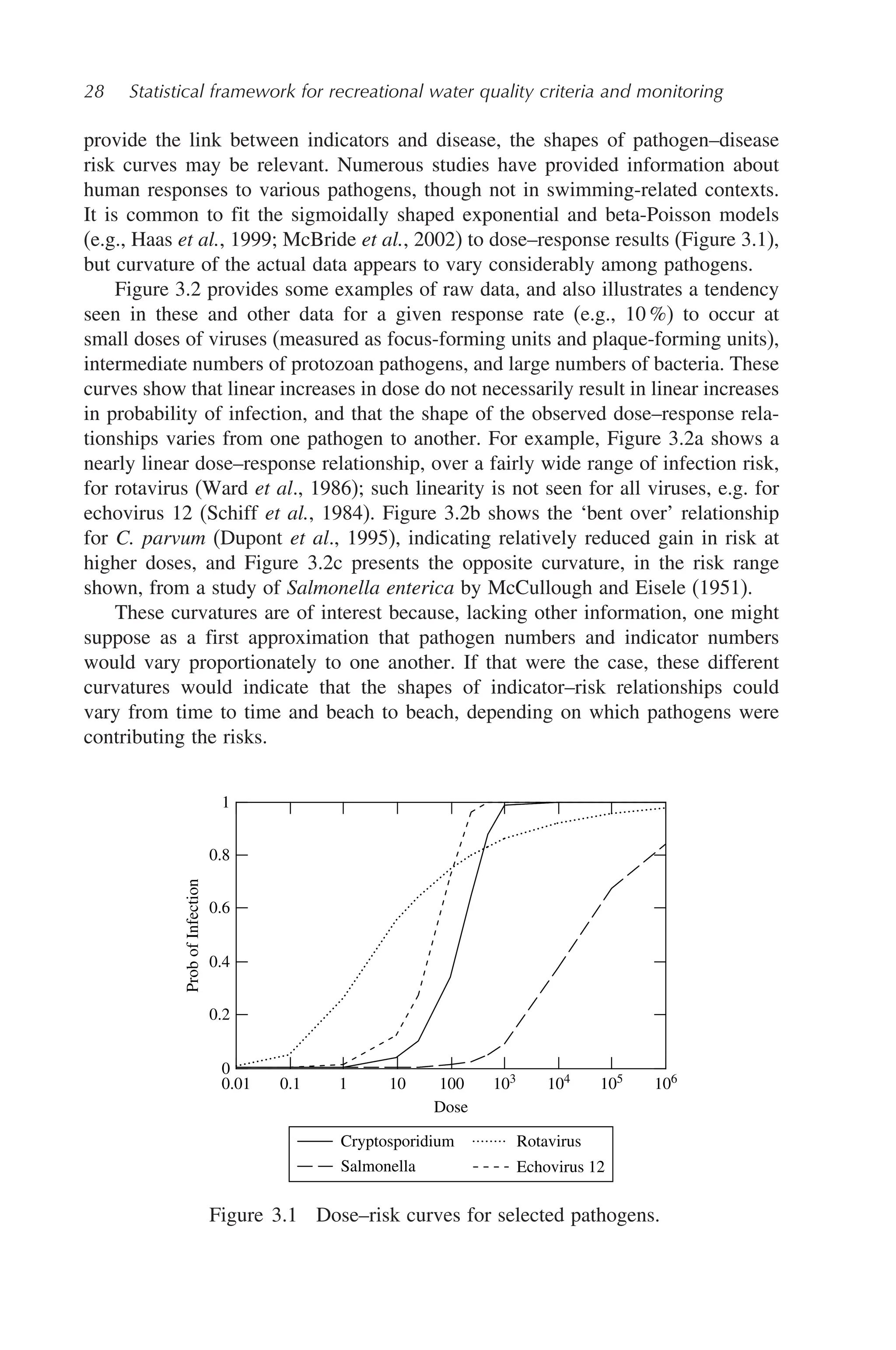
Figure 3.2 Example dose–risk curves for (a) viral (rotavirus; Ward et al., 1986),
(b) protozan (C. parvum; Dupont et al., 1995), and (c) bacteria (S.enterica Var
meleagridis, strain III; McCullough and Eiselk, 1951) pathogens. In each case, one
or more high points has been omitted, to emphasize the forms of the relationships
at lower risk levels of interest in protecting swimmers. ffu: focus-forming units.
3.4 Similarities and differences between pathogens
and indicators
Indicator bacteria and pathogenic microbes may differ in several ways that could
reduce the ability of the indicators to predict pathogen levels. Some possibilities are:
• die-off rates from sunlight, heat, salt, or other qualities of water;
• reductions of concentrations and viability from water treatment processes;
• loss to predation by zooplankton;
• sedimentation rates.
Brookes et al. (2004) discussed the complexity of pathogens being transported
into lakes and reservoirs by rivers, considering that pathogens could settle to the
bottom, or be inactivated by heat, ultraviolet light, and grazing by predators. Indi-
cator bacteria could easily differ from pathogenic microbes in each of those ways.
Skraber et al. (2004) compared coliform bacteria and coliphage viruses as indica-
tors of viral contamination in river water. They found that ‘the number of virus
genome-positive samples decreased with decreasing concentration of coliphages,
while no such relation was observed for thermotolerant coliforms’. The relationship
between coliforms and pathogenic viruses varied with water temperature.
It would be interesting to know the differences between pathogens and indicators
in their tendencies to be carried by water, their sedimentation rates, and their
survival in waters of different types. Indicator bacteria are thought to die off faster
in bright sun (Wymer et al., 2004). For example, literature values indicate die-off
rates for total coliform in darkness of 0–0.1 hr−1
(Hydroscience 1977) and in peak
sunlight of 1.5–4.6 hr−1
(Fujioka et al., 1981). A study by Noble and Fuhrman](https://image.slidesharecdn.com/2156211-250607125537-41ccaf7f/75/Statistical-Framework-For-Recreational-Water-Quality-Criteria-And-Monitoring-Larry-J-Wymer-42-2048.jpg)