ขั้นตอนต่อไป กด addfolder เพื่อเอางานในไฟล์ จากนั้นกด save
จากนั้นกด เพื่อเลือกไฟล์ DEM
3.
จากนั้นใส่ตัวแปร คาว่า DEM= GRIDobj('kidchakood.tif') แล้วกด Enter แล้วพิมคาว่า imagesc(DEM)
แล้วกด Enter จะรูปออกมาเป็นแบบข้างล่าง
รูปที่ได้จากการใส่ตัวข้างบน
4.
จากนั้นเราอยากเห็นกราฟที่เป็น hill shadeแล้วก็พิมพ์คาว่าimageschs(DEM,min(gradient8(DEM),1))แล้ว
กด Enter จะรูปออกมาเป็นแบบข้างล่าง
Plot (กราฟ)
ประกาศตัวแปร x y
RGB triplet คือแม่สีหลัก
[ 0 0 0 ]
R G B เป็น 0 หมดคือสีดา
[ 1 1 1 ]
R G B เป็น 1 คือสีขาว
ถ้าอยากทาให้เป็นสีชมพูต้องนาสีแดงผสมกับสีขาว จะได้
[0.2 1 1]
R G B
ใส่คาอธิบายสัญลักษณ์ ใช้คาสั่ง legend('score of classroom')
การทาการไหลของน้า เราอย่าลืมคานี้ DEMf= fillsinks(DEM); เพราะว่าถ้าลืมจะเกิดร่องน้าแล้วพิมพ์คานี้
ต่อ
FD = FLOWobj(DEMf);
A = flowacc(FD);
imageschs(DEM,dilate(sqrt(A),ones(5)),'colormap',flipud(copper)); จากนั้นกด Enter จะได้รูปข้างล่าง
การใช้ drainagebasins
เราพิมพ์ DB = drainagebasins(FD);
DB = shufflelabel(DB);
nrDB = numel(unique(DB.Z(:)))-1; % nr of drainage basins
STATS = regionprops(DB.Z,'PixelIdxList','Area','Centroid');
imageschs(DEM,DB);
hold on
for run = 1:nrDB;
if STATS(run).Area*DB.cellsize^2 > 10e6;
figure;
imshowpair(I1,I2,'ColorChannels','red-cyan');
title('Composite Image (Red- Left Image, Cyan - Right Image)');
blobs1 = detectSURFFeatures(I1, 'MetricThreshold', 2000);
blobs2 = detectSURFFeatures(I2, 'MetricThreshold', 2000);
figure;
imshow(I1);
hold on;
plot(selectStrongest(blobs1, 30));
title('Thirty strongest SURF features in I1');
figure;
imshow(I2);
hold on;
plot(selectStrongest(blobs2, 30));
title('Thirty strongest SURF features in I2');
[features1, validBlobs1] = extractFeatures(I1, blobs1);
[features2, validBlobs2] = extractFeatures(I2, blobs2);
indexPairs = matchFeatures(features1, features2, 'Metric', 'SAD', ...
'MatchThreshold', 5);
matchedPoints1 = validBlobs1(indexPairs(:,1),:);
matchedPoints2 = validBlobs2(indexPairs(:,2),:);
figure;
showMatchedFeatures(I1, I2, matchedPoints1, matchedPoints2);
legend('Putatively matched points in I1', 'Putatively matched points in I2');
[fMatrix, epipolarInliers, status] = estimateFundamentalMatrix(...
matchedPoints1, matchedPoints2, 'Method', 'RANSAC', ...
'NumTrials', 10000, 'DistanceThreshold', 0.1, 'Confidence', 99.99);
if status ~= 0 || isEpipoleInImage(fMatrix, size(I1)) ...
|| isEpipoleInImage(fMatrix', size(I2))
error(['Either not enough matching points were found or '...
35.
'the epipoles areinside the images. You may need to '...
'inspect and improve the quality of detected features ',...
'and/or improve the quality of your images.']);
end
inlierPoints1 = matchedPoints1(epipolarInliers, :);
inlierPoints2 = matchedPoints2(epipolarInliers, :);
figure;
showMatchedFeatures(I1, I2, inlierPoints1, inlierPoints2);
legend('Inlier points in I1', 'Inlier points in I2');
[t1, t2] = estimateUncalibratedRectification(fMatrix, ...
inlierPoints1.Location, inlierPoints2.Location, size(I2));
tform1 = projective2d(t1);
tform2 = projective2d(t2);
I1Rect = imwarp(I1, tform1, 'OutputView', imref2d(size(I1)));
I2Rect = imwarp(I2, tform2, 'OutputView', imref2d(size(I2)));
% transform the points to visualize them together with the rectified images
pts1Rect = transformPointsForward(tform1, inlierPoints1.Location);
pts2Rect = transformPointsForward(tform2, inlierPoints2.Location);
figure;
showMatchedFeatures(I1Rect, I2Rect, pts1Rect, pts2Rect);
legend('Inlier points in rectified I1', 'Inlier points in rectified I2');
Irectified = cvexTransformImagePair(I1, tform1, I2, tform2);
figure;
imshow(Irectified);
title('Rectified Stereo Images (Red - Left Image, Cyan - Right Image)');
cvexRectifyImages('lions_left.jpg', 'lion_right.jpg');


![RGB triplet คือ แม่สีหลัก
[ 0 0 0 ]
R G B เป็น 0 หมดคือสีดา
[ 1 1 1 ]
R G B เป็น 1 คือสีขาว
ถ้าอยากทาให้เป็นสีชมพูต้องนาสีแดงผสมกับสีขาว จะได้
[0.2 1 1]
R G B
ใส่คาอธิบายสัญลักษณ์ ใช้คาสั่ง legend('score of classroom')](https://image.slidesharecdn.com/random-160501073315/85/slide-10-320.jpg)


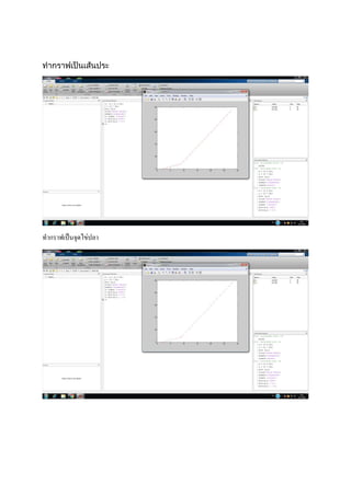
![กราฟ 3 มิติ
เราจะให้กราฟเป็น 3มิติ ให้เราพิมพ์คาว่าลงไปในโปรแกรม DEMc = crop(DEM,sub2ind(DEM.size,[150
350],[150 350])); )) แล้วกด Enter](https://image.slidesharecdn.com/random-160501073315/85/slide-16-320.jpg)
![จากนั้นพิมพ์ เพื่อให้อยู่ในรูปของตัวเลข[Z,x,y] = GRIDobj2mat(DEMc); แล้วกด Enterแล้วพิมพ์คานี้ต่อ
surf(x,y,double(Z)) เราก็จะได้รูปเป็น 3ติ แล้วเหมือนรูปข้างล่างค่ะ
รูป 3มิติที่เราใส่ตัวแปรลงไป](https://image.slidesharecdn.com/random-160501073315/85/slide-17-320.jpg)


![[x,y] = ind2coord(DB,...
sub2ind(DB.size,...
round(STATS(run).Centroid(2)),...
round(STATS(run).Centroid(1))));
text(x,y,...
num2str(round(STATS(run).Area * DB.cellsize^2/1e6)),...
'BackgroundColor',[1 1 1]);
end
end
hold off
title('drainage basins (numbers refer to drainage basin area in km^2)') แล้วกด Enter จะได้ตามรูปข้างล่าง](https://image.slidesharecdn.com/random-160501073315/85/slide-20-320.jpg)


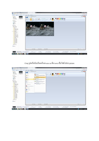


![figure;
imshowpair(I1,I2,'ColorChannels','red-cyan');
title('Composite Image (Red - Left Image, Cyan - Right Image)');
blobs1 = detectSURFFeatures(I1, 'MetricThreshold', 2000);
blobs2 = detectSURFFeatures(I2, 'MetricThreshold', 2000);
figure;
imshow(I1);
hold on;
plot(selectStrongest(blobs1, 30));
title('Thirty strongest SURF features in I1');
figure;
imshow(I2);
hold on;
plot(selectStrongest(blobs2, 30));
title('Thirty strongest SURF features in I2');
[features1, validBlobs1] = extractFeatures(I1, blobs1);
[features2, validBlobs2] = extractFeatures(I2, blobs2);
indexPairs = matchFeatures(features1, features2, 'Metric', 'SAD', ...
'MatchThreshold', 5);
matchedPoints1 = validBlobs1(indexPairs(:,1),:);
matchedPoints2 = validBlobs2(indexPairs(:,2),:);
figure;
showMatchedFeatures(I1, I2, matchedPoints1, matchedPoints2);
legend('Putatively matched points in I1', 'Putatively matched points in I2');
[fMatrix, epipolarInliers, status] = estimateFundamentalMatrix(...
matchedPoints1, matchedPoints2, 'Method', 'RANSAC', ...
'NumTrials', 10000, 'DistanceThreshold', 0.1, 'Confidence', 99.99);
if status ~= 0 || isEpipoleInImage(fMatrix, size(I1)) ...
|| isEpipoleInImage(fMatrix', size(I2))
error(['Either not enough matching points were found or '...](https://image.slidesharecdn.com/random-160501073315/85/slide-34-320.jpg)
!['the epipoles are inside the images. You may need to '...
'inspect and improve the quality of detected features ',...
'and/or improve the quality of your images.']);
end
inlierPoints1 = matchedPoints1(epipolarInliers, :);
inlierPoints2 = matchedPoints2(epipolarInliers, :);
figure;
showMatchedFeatures(I1, I2, inlierPoints1, inlierPoints2);
legend('Inlier points in I1', 'Inlier points in I2');
[t1, t2] = estimateUncalibratedRectification(fMatrix, ...
inlierPoints1.Location, inlierPoints2.Location, size(I2));
tform1 = projective2d(t1);
tform2 = projective2d(t2);
I1Rect = imwarp(I1, tform1, 'OutputView', imref2d(size(I1)));
I2Rect = imwarp(I2, tform2, 'OutputView', imref2d(size(I2)));
% transform the points to visualize them together with the rectified images
pts1Rect = transformPointsForward(tform1, inlierPoints1.Location);
pts2Rect = transformPointsForward(tform2, inlierPoints2.Location);
figure;
showMatchedFeatures(I1Rect, I2Rect, pts1Rect, pts2Rect);
legend('Inlier points in rectified I1', 'Inlier points in rectified I2');
Irectified = cvexTransformImagePair(I1, tform1, I2, tform2);
figure;
imshow(Irectified);
title('Rectified Stereo Images (Red - Left Image, Cyan - Right Image)');
cvexRectifyImages('lions_left.jpg', 'lion_right.jpg');](https://image.slidesharecdn.com/random-160501073315/85/slide-35-320.jpg)