This document summarizes research on improving the resistance of concrete to freezing and thawing. It includes three parts: Part I examines factors related to the paste portion of concrete and evaluates test methods to assess air void systems and water pore systems. Laboratory testing was conducted on concrete mixtures with durable aggregate. Part II investigates factors related to the coarse aggregate portion and introduces the Washington Hydraulic Fracture Test to identify frost-susceptible aggregates. Part III summarizes field testing programs to evaluate paste mixtures and methods to mitigate existing cracking from frost-susceptible aggregates. Preliminary results are also presented.

1. SHRP-C-391
Resistance of Concrete
to Freezing and Thawing
Donald J. Janssen
University of Washington
Seattle, Washington 98195
Mark B. Snyder
University of Minnesota
Minneapolis, Minnesota 55455
Strategic Highway Research Program
National Research Council
Washington, DC 1994

2. SHRP-C-391
Contract C-203
ISBN 0-309-05773-6
Product no. 2002, 2004, 2018, 2019, 2020, 2021
Program Manager: Don M. Harriott
Project Manager: Inam Jawed
Editor: Katharyn L. Bine
Production Editors: Carina S. Hreib, Carrie Kent
June 1994
key words:
aggregate
D-cracking
durability factor
freezing and thawing
modal analysis
portland cement concrete
quality factor
resonance frequency
Strategic Highway Research Program
National Research Council
2101 Constitution Avenue N.W.
Washington, DC 20418
(202) 334-3774
The publication of this report does not necessarily indicate approval or endorsement by the National Academy of
Sciences, the United States Government, or the American Association of State Highway and Transportation
Officials or its member states of the findings, opinions, conclusions, or recommendations either inferred or
specifically expressed herein.
©1994 National Academy of Sciences
1.5M/NAP/694

3. Acknowledgments
The research described herein was supported by the Strategic Highway Research Program
(SHRP). SHRP is a unit of the National Research Council that was authorized by section
128 of the Surface Transportation and Uniform Relocation Assistance Act of 1987.
This book represents the efforts of many people and organizations. Appendix D, "Damping
Measurements for Nondestructive Evaluation of Concrete Beams," was a collaborative work
by Elizabeth A. Vokes, Washington State Department of Transportation; Steven L. Clarke,
Archos, Inc.; Donald J. Janssen, University of Washington; and the Washington State
Transportation Center (TRAC). The National Science Foundation provided some of the Test
Equipment used in this particular study. J. D. Chalupnik and D. W. Storti, Department of
Chemical Engineering, and W. D. Scott, Department of Material Science and Engineering
assisted in the development of the initial impulse-excitation procedures. Additional support
came from the National Science Foundation and in-kind support from Michigan State
University and the University of Washington.
iii

4. Preface
The mechanisms of damage to concrete from repeated cycles of freezing and thawing are not
well understood and continue to be intensively studied. Original research was based on the
fact that water expands 9 percent when it freezes. Thus, the term "critical saturation" was
coined to describe the point at which the concrete pores were 91.7 percent saturated and,
therefore, assumed to be susceptible to damage due to freezing and thawing. Further
investigation determined that deterioration due to freezing and thawing can affect concrete
with lower degrees of saturation.1
Four theories have gained wide acceptance in describing the mechanisms of frost action. 2
Although most of these theories were originally used to describe the frost action in cement
paste, they are also applicable to concrete. 3The first was the hydraulic pressure theory
Powers proposed in 1945. This was followed by the diffusion and growth of capillary ice
theory constructed by Powers and Helmuth in 1953, the dual mechanism theory by Larson
and Cady in 1969, and the desorption theory by Litvan in 1972. Other theories have been
proposed, but these four form the basis of most research in the area of frost resistance of
concrete.
Powers' hydraulic pressure theory proposes that destructive stresses can develop if water is
displaced to accommodate the advancing ice front in concrete. 4 If the pores are critically
saturated, water will begin to flow to make room for the increased ice volume. Hydraulic
pressures generated during the water flow will be dependent upon the length of the flow
path, the rate of freezing, the permeability of the concrete, and the viscosity of the water.
The concrete will rupture if the hydraulic pressure exceeds its tensile strength.
Further studies by Powers and Helmuth revealed that the hydraulic pressure theory did not
account for continued dilation of some specimens and shrinkage of other specimens at a
constant temperature, s They therefore proposed that the production of ice produces a
relatively concentrated alkali solution at the freezing site. Unfrozen water will, in turn,
move toward the site because of the differences in solute concentrations in a process similar
to osmosis. Hence, the pressure developed was called osmotic pressure.
Larson and Cady produced results that they felt were supported by the hydraulic pressure
theory. 6 However, they also noted continued dilation of concrete specimens after the
equipment indicated that freezing had ceased. They attributed these dilations to the hydraulic
pressures generated by the increase in the specific volume of water during the "ordering," or
change of state, from bulk water on the ice and pore surfaces to adsorbed water.
V

5. Litvan's desorption theory proposes that vapor pressure differentials, created as the relative
humidity decreases in the aggregate pores, force water to migrate out of the aggregate pore. 7
As in Powers' theory, the concrete will rupture if the hydraulic pressures generated during
migration exceed the tensile strength of the concrete.
While these theories disagree as to whether water moves toward or away from the point of
ice formation, they agree that the amount of water in the pores and the resistance to
movement of that water play a role in the frost resistance of concrete. In the case of
concrete, it is generally accepted that the pore system is potentially susceptible to damage
from freezing and thawing. Efforts to produce frost-resistant concrete have primarily
focused on providing a proper system of entrained air voids. In the case of aggregates, some
pore systems do not show susceptibility to damage from freezing and thawing while other
pore systems do. In addition to the air-entrainment of concrete as mentioned above, efforts
have also focused on identifying the aggregates with acceptable pore systems for use in
concrete exposed to freezing and thawing.
The work is presented in three parts: Part I, which deals with those factors that relate
primarily to the paste portion of the concrete; Part II, which deals with those factors
primarily relating to the coarse aggregate portion of the concrete; and Part III, which
summarizes and presents preliminary results of the field work for Parts I and II. The first
chapter of each part begins with a full description of the scope of the part. The data and
other information presented in each part are given in separate appendices.
vi

6. References
1. Powers, T. C. "Freezing Effects In Concrete," American Concrete Institute SP 47-1,
1975, pp. 1-11.
2. Thompson, S. R., M. P. Olsen and B. J. Dempsey. "D-Cracking in Portland Cement
Concrete Pavements," 1980, Project IHR-413.
3. Verbeck, G. and R. Landgren. "Influence of Physical Characteristics of Aggregates on
Frost Resistance of Concrete," ASTM Proceedings, Vol. 60, 1960, pp. 1063-1079.
4. Powers, T. C. "A Working Hypothesis for Further Studies of Frost Resistance of
Concrete," Journal of the American Concrete Institute, Vol. 16, No. 4, 1945, pp. 245-
272.
5. Powers, T. C. and R. A. Helmuth. "Theory of Volume Changes in Hardened Portland-
Cement Paste During Freezing," Highway Research Board Proceedings, Vol. 32, 1953,
pp. 285-297.
6. Larson, T. D. and P. D. Cady. "Identification of Frost-Susceptible Particles in Concrete
Aggregates," NCHRP Report 66, 1969.
7. Litvan, G. G. "Phase Transitions of Adsorbates, IV, Mechanism of Frost Action in
Hardened Cement Paste," American Ceramic Society Journal, Vol. 55, No. 1, 1972, pp.
38-42.
vii

7. Contents
Part I - Frost Resistance of Concrete Made with Durable Aggregate
1.0 Introduction .............................................. 1
1.1 Background ........................................... 1
1.2 Objectives ........................................... 1
2.0 Laboratory Testing Program .................................... 1
2.1 Purpose ............................................. 1
2.2 Test Matrices ......................................... 2
2.3 Air Void System Evaluation ................................. 3
2.4 Water Pore System Evaluation ............................... 3
2.5 Freezing and Thawing Test Procedure .......................... 6
3.0 Innovative Test Procedures ..................................... 7
3.1 Modification of AASHTO T 161 (ASTM C 666) .................... 7
3.2 Modification of ASTM C 215 ............................... 8
4.0 Results ................................................ 10
5.0 Acceptable Variability and Maximum Expected Errors in Results ............ 10
5.1 Variability of Durability Factor Results ......................... 10
5.2 Maximum Errors in Linear Traverse Results ..................... 10
5.3 Reliability of Freezable Moisture Results ........................ 14
6.0 Frost-Resistance Model ...................................... 14
7.0 Summary and Recommendations for Part I .......................... 14
7.1 Test Procedures ....................................... 15
7.2 Durability Data Base .................................... 15
7.3 Recommendations ...................................... 15
ix

8. References ................................................ 17
Appendix A. Design Matrices ..................................... 19
Appendix B. Proposed Modifications to AASHTO T 161
Standard Method of Test for Resistance of Concrete
to Rapid Freezing and Thawing .................................. 23
Appendix C. Standard Test Method for Determining the Fundamental
Transverse Frequency and Quality Factor of
Concrete Prism Specimens .................................... 35
Appendix D. Damping Measurements for Nondestructive
Evaluation of Concrete Beams .................................. 45
Appendix E. Tabulated Results . . . ................................. 67
Part II - Frost Resistance of Concrete Made with Frost-Susceptible Aggregate
1.0 Introduction ............................................. 79
2.0 Background ............................................. 79
2.1 D-Cracking Occurrence ...................................... 79
2.2 Conditions Necessary for D-cracking ............................. 79
3.0 Current Identification Procedures ................................ 80
3.1 Environmental Simulation Tests ............................. 80
3.1.1 Sulfate Soundness (AASHTO T104) ...................... 81
3.1.2 Unconfined Aggregate Freezing and Thawing (AASHTO T103) ..... 81
3.1.3 Rapid Freezing and Thawing (AASHTO T161) ............... 81
3.1.4 Powers Slow Cool (ASTM C671) ....................... 82
3.1.5 Single-Cycle Slow Freeze ............................ 82
3.2 Aggregate Index Property Tests ............................. 83
3.2.1 Mercury Intrusion Porosimeter ......................... 83
3.2.2 Iowa Pore Index Test ............................... 83
3.2.3 Absorption-Adsorption .............................. 84
3.2.4 Petrographic Analysis (ASTM C295) ..................... 84
X

9. 4.0 Washington Hydraulic Fracture Test .............................. 85
4.1 Objectives .......................................... 85
4.2 Test Description ....................................... 85
4.3 Test Mechanism ....................................... 85
4.4 Equipment .......................................... 87
4.5 Test Procedure ........................................ 90
4.6 Analysis of Results ..................................... 90
4.6.1 Calculations ..................................... 91
4.6.2 Pressure Effect ................................... 92
4.6.3 Aggregate Size Effect ............................... 92
4.7 Reliability and Repeatability ............................... 92
4.8 Chamber Modification ................................... 93
5.0 Mitigation of Existing D-Cracking ............................ 97
5.1 Preventing Freezing .................................... 102
5.2 Reducing Moisture .................................... 102
References ............................................... 106
Appendix 2A Washington Hydraulic Fracture Test
Procedure AASHTO Test Procedure Format ........................ 109
Appendix 2B Assembling and Operating the Washington Hydraulic
Fracture Test Apparatus: Large Chamber .......................... 121
Part IlI - Field Testing Program
1.0 Introduction ............................................ 127
2.0 Paste Test Program ....................................... 127
2.1 Objectives ......................................... 127
2.2 Test Program Design ................................... 127
2.2.1 Site Selection ................................... 127
2.2.2 Mixture Selection ................................. 128
2.2.3 Ohio Test Site Experimental Design Details ................. 128
2.2.4 Minnesota Test Site Experimental Design Details ............. 133
2.3 Construction Summaries .................................. 137
xi

10. 2.4 Monitoring Program ................................... 138
2.4.1 Construction Monitoring ............................. 138
2.4.2 Performance Monitoring ............................. 139
2.5 Laboratory Tests ..................................... 140
2.6 Preliminary Findings ................................... 146
3.0 D-Crack Mitigation Test Program .............................. 147
3.1 Objectives ......................................... 147
3.2 Test Program Design ................................... 147
3.3 Construction Summaries ................................. 148
3.4 Monitoring Program ................................... 149
3.5 Laboratory Tests ..................................... 149
3.6 Laboratory Test Results ................................. 150
3.6.1 Water-based Silane Treatment ......................... 150
3.6.2 Solvent-based Silane Treatment ........................ 153
3.6.3 Penetrating Oil Treatment ............................ 155
3.6.4 Two-Part Resin Surface Sealer Treatment .................. 155
3.6.5 Summary of Laboratory Test Results ..................... 158
4.0 Other Field Mixes ........................................ 159
4.1 Background ......................................... 159
4.2 Testing Summary ..................................... 159
5.0 Conclusions and Summary ................................... 159
Appendix A Freezing and Thawing Test Histories for Ohio Test Mixtures ..... 161
Appendix B Freezing and Thawing Test Histories for Minnesota Test Mixtures . . 185
xii

11. List of Figures
Part I
Figure 1-1 Moisture Content versus E_luilibrium Relative Humidity ............. 5
Figure 1-2 Variability of AASHTO T161 Procedures .................... 12
Figure 1-3 Maximum Error of Linear Traverse Air Content ................ 12
Figure 1-4 Maximum Error of Spacing Factor ......................... 13
Figure 1-5 Maximum Error of Specific Surface ........................ 13
Figure D-1 Idealized Frequency Response Curve ....................... 49
Figure D-2 Typical Nyquist Plot ................................. 52
Figure D-3 Schematic of Test Setup ............................... 54
Figure D-4 Changes in Relative Dynamic Modulus ...................... 56
Figure D-5 Changes in Relative Q ................................ 56
Figure D-6 Q-Failure Cycle versus Cycles to 60 percent RDM ............... 57
Part II
Figure 2-1 Winslow Absorption Rates for Four Aggregates ................. 88
Figure 2-2 Winslow Absorption Rates for Silane-Treated
and ILA Crashed Limestone ............................. 89
Figure 2-3 Comparison of Percent Fractures for plus 19.0 mm (3/4 in.)
Durable Gravel, at both 7240 kPa (1050 psi)
and 7930 kPa (1150 psi) Testing Pressures .................... 94
oo.
XIII

12. Figure 2-4 Comparison of Percent Fractures for plus 19.0 mm (3/4 in.)
Nondurable Gravel, at both 7240 kPa (1050 psi)
and 7930 kPa (1150 psi) Testing Pressures .................... 94
Figure 2-5 Comparison of Percent Fractures for plus 19.0 mm (3/4 in.)
and minus 19.0 mm Durable Gravel ........................ 98
Figure 2-6 Comparison of Percent Fractures for plus 19.0 mm (3/4 in.)
and minus 19.0 mm Nondurable Gravel ...................... 98
Figure 2-7 Pressure Release Rate History for Original Chamber .............. 99
Figure 2-8 Pressure Release Histories for Original and Large Chambers ........ 100
Figure 2-9 The Large Washington Hydraulic Fracture Test Apparatus ......... 101
xiv

13. List of Tables
Part I
Table 1-1 Relative Humidity at 25°C for Selected Saturated Salt Solutions ......... 4
Table 1-2 Summary of Rapid Test Method Comparisons .................... 7
Table 1-3 Comparison of Precision between ASTM C215
and the "Proposed Fundamental Transverse Frequency
and Quality Factor of Concrete Prism Specimens" ................. 9
Table 1-4 Comparison of DF Variability for Two Methods
of Measuring Fundamental Transverse Frequency .................. 9
Table A-1 Preliminary Tests for Statistical Calibration
and Normal Concretes (Matrix A) .......................... 19
Table A-2 Water Reducer and Air-Entraining Admixture Type (Matrix B) ........ 19
Table A-3 Cement and Aggregate Types,
including SHRP C-205 HES Mixes (Method C) .................. 20
Table A-4 Pozzolanic Admixtures (Matrix D) .......................... 20
Table A-5 Pozzolan Amount and Curing Period (Matrix E) .................. 21
Table A-6 List of Admixtures .................................... 22
Table D-1 Typical Value for Relative Dynamic Modulus
and Quality Factor Measurements ........................... 58
Table D-2 Q-Failure and Actual Failure Cycle, Single Beam from Each Mix Tested . . 59
Table D-3 Q-Failure and Cycles to 60 Percent RDM,
Average of Five Beams from Each Mix Tested .................. 60
XV

14. Table D-4 Q-Failure Determined Prior to 60 Percent RDM
and Cycles 60 Percent RDM, Average of Five Beams
from Each Mix Tested ................................. 63
Table D-5 Predicted and Actual Durability Factors ....................... 64
Part II
Table 2-1 WHFT Results, > 19 mm (3/4 in.) Size ...................... 95
Table 2-2 Effect of Sample Size on Variability ......................... 96
Table 2-3 Between Laboratory Results .............................. 96
Table 2-4 Effect of Asphalt Overlay Thickness on Reducing Freezing
in Concrete Pavement ................................. 103
Table 2-5 Durability Factors of Sealer Tested Cores
from D-Cracking to Pavement Susceptibility ................... 104
Part Ill
Table 3-1 Summary of Field Mixtures used on Ohio D-Cracking
Test Road Site (Cast 9/1/92 to 9/11/92) ...................... 130
Table 3-2 Raw Material Properties for Ohio Field Tests .................. 131
Table 3-3 Layout of SHRP Concrete Frost Resistance Program Repairs
and Concrete Sealers in Ohio ............................ 132
Table 3-4 Summary of Field Mixtures used at the Minnesota Road Research Site
(Cast 10/15/92) ..................................... 135
Table 3-5 Raw Material Properties for Minnesota Field Tests ............... 136
Table 3-6 Summary of Laboratory Compression Test Results
on the Materials from the Ohio D-Cracking Test Road Site
(Cast 9/1/92 to 9/11/92) ............................... 141
Table 3-7 Summary of Laboratory Compression Test Results
on Materials from the Minnesota Road Research Site (Cast 10/15/92) .... 141
Table 3-8 Summary of Laboratory Durability Test Results
Ohio D-Cracking Test Road Site (Cast 9/1/92 to 9/11/92) ........... 142
xvi

15. Table 3-9 Summary of Laboratory Durability Test Results
from the Minnesota Road Research Site (Cast 10/15/92) ............ 143
Table 3-10 Summary of Laboratory Durability Test Results
from the Ohio D-Cracking Test Road Site (Cast 9/1/92 to 9/11/92) ..... 144
Table 3-11 Summary of Laboratory Durability Test Results
from the Minnesota Road Research Site (Cast 10/15/92) ............ 145
Table 3-12 Ohio Core Measurements and D-Cracking Mitigation Treatments ...... 151
Table 3-13 Results of Freeze-Thaw Testing of
D-Cracking Susceptible Concrete Treated with Water-based Silane ..... 152
Table 3-14 Significance Levels and Confidence Intervals
for Results of Freeze-Thaw Testing of D-Cracking
Susceptible Concrete Treated with Water-based Silane ............. 152
Table 3-15 Results of Freeze-Thaw Testing of D-Cracking
Susceptible Concrete Treated with Solvent-based Silane ............ 154
Table 3-16 Significance Levels and Confidence Intervals for Results
of Freeze-Thaw Testing of D-Cracking Susceptible Concrete
Treated with Solvent-based Silane ......................... 154
Table 3-17 Results of Freeze-Thaw Testing of D-Cracking
Susceptible Concrete Treated with Penetrating Oil Sealer ........... 156
Table 3-18 Significance Levels and Confidence Intervals for Results
of Freeze-Thaw Testing of D-Cracking Susceptible Concrete
Treated with Penetrating Oil Sealer ......................... 156
Table 3-19 Results of Freeze-Thaw Testing of D-Cracking
Susceptible Concrete Treated with Two-Part Resin Surface Sealer ...... 157
Table 3-20 Significance Levels and Confidence Intervals for Results
of Freeze-Thaw Testing of D-Cracking Susceptible Concrete
Treated with Two-Part Resin Surface Sealer ................... 157
xvii

16. Abstract
This study, aimed at improving the freeze-thaw resistance of concrete, consists of three parts.
Part I evaluates parameters affecting the freeze-thaw durability of concrete. A modification
of the existing standard of method for determining the durability factor of concrete specimens
is proposed, and a new procedure for fundamental transverse frequency (used in durability
factor calculations) has been developed. Part II focuses on developing better methods for
identifying nondurable aggregates, and has resulted in a rapid new test based on the hydraulic
fracture of aggregates. Part III describes field experiments to evaluate the freeze-thaw
resistance of a number of specified concrete mixes and the use of sealants to mitigate D-
cracking. Preliminary field performance results are presented.
xix

17. Executive Summary
This document summarizes the results of a four-year program of research into the resistance
of concrete to freezing and thawing. The work is presented in three parts. Part I is a
discussion of factors primarily relating to the paste portion of the concrete. Part II relates
primarily to the coarse aggregate portion of the concrete. Part III summarizes preliminary
results for the field work relating to Parts I and II. The appendices contain the data and
other information supplemental to the parts. These three parts are summarized below:
Part I: Frost Resistance of Concrete Made with Durable Aggregate
A revised test procedure and a new test procedure for concrete made with durable (frost-
resistant) aggregate by rapid freezing and thawing is presented. Durability factor (DF) was
measured for a variety of mix parameters, with the emphasis being placed on identifying mix
combinations that produced DF values in the 25 to 75 range. Air-void parameters were
measured by linear traverse. The water pore systems were evaluated by permeability
measurement and by determining the theoretical amount of water that would freeze at -18°C
(called freezable moisture in the text).
A modification to AASHTO T 161 was developed to address concerns with current variations
of AASHTO T 161 regarding container restraint in Procedure A and specimen drying in
Procedure B. The modification consists of wrapping the specimens in terrycloth to keep
them moist during freezing without needing containers. The modification is slightly more
severe than current procedures, and shows less variability in results.
A new procedure for determining fundamental transverse frequency (used to calculate DF)
was developed. The procedure consists of causing a specimen to vibrate by impacting it with
an instrumented hammer, then evaluating the frequency response spectrum measured with an
accelerometer. The procedure is more than an order of magnitude more precise than the
published precision for the current method of determining fundamental transverse frequency,
ASTM C 215. No frost resistance models were developed because insufficient freezable
moisture data was available to permit adequate modelling.
Part II: Frost Resistance of Concrete Made with Frost-Susceptible
Aggregate
The primary focus of this part was to develop a new test procedure for identifying aggregates
which are not durable when subjected to freezing and thawing in concrete (D-cracking
xxi

18. susceptible). The procedure, called the Washington Hydraulic Fracture Test, uses
compressed gas to force water into the pores of a dry aggregate. When the pressure is
released, the aggregate must dissipate internal pressure. Aggregate that cannot dissipate the
pressure rapidly fracture. The amount of fracturing is determined, and a value called the
hydraulic fracture index (HFI) is calculated. This value is an estimate of the number of
pressurization cycles necessary to produce 10 percent of the pieces of aggregate to fracture.
The laboratory results were compared to reports of field performances. Aggregates with
high (80 to 100 or higher) HFI values tended to be non-D-cracking susceptible, while
aggregates with low (less than about 60) HFI values tended to be D-cracking susceptible.
Mitigation for existing D-cracking was also investigated. Findings suggested that the most
suitable method of treating existing D-cracked pavements would be to replace the concrete
with a full-depth patch. Prior to placing the new concrete, the exposed face of the existing
concrete section should be sealed to prevent moisture intrusion. This method would only be
appropriate for pavements and other concrete with considerable intact concrete away from
joints and cracks. This mitigation method is evaluated in Part III.
Part III: Field Studies
Several questions arose from the work reported in Parts I and II of this report relating to
field performance, namely: 1) how the newly-developed modification of AASHTO T 161
relates to field performance; 2) whether non-traditional mixes (such as mixes containing
pozzolans or very high cement contents) follow the same accepted criteria for resistance to
freezing and thawing as traditional air-entrained mixes; and 3) whether the progression of
field D-cracking can be slowed sufficiently to significantly extend the life of pavements
containing D-cracking susceptible aggregates. These questions were addressed by the
construction of field test sections.
Full-depth concrete patches made with a range of high-performance materials (high cement
contents, accelerators, and blended cements used to achieve specified early-opening
strengths) were placed. The concrete patches had a range of air contents to produce an
expected range of performance. Companion specimens from many of the mixes produced
laboratory DF values less than 60, and would be expected to fail. These test patches require
further monitoring to evaluate field performance.
Test slabs containing varying amounts of fly ash were placed in Minnesota with a range of
air contents to produce an expected range of performance. Companion specimens from most
of the mixes produced DF values above 90, even though the air-void systems would be
judged to be substandard by conventional wisdom. Further field monitoring will be needed
to evaluate field performance of these sections. Many of the patches in Ohio were placed in
pavements made with aggregates susceptible to D-cracking. Prior to placing the new
concrete, the cut faces of the existing concrete received one of a variety of sealer treatments.
Field monitoring will be needed to evaluate differences in field performance of the sealer
treatments.
xxii

19. Part I - Frost Resistance of Concrete Made with Durable
Aggregate
1.0 Introduction
1.1 Background
Frost resistance of concrete made with durable aggregate is determined by the air-void
system's ability to prevent development of destructive pressures due to freezing and
associated movement of moisture in the concrete pores. The specific requirements of the
air-void system depend on the amount and mobility of the water in the pores. An
investigation of the frost resistance of concrete made with durable aggregates should identify
the air-void system necessary to protect a variety of concrete water-pore systems.
1.2 Objectives
The goal of this research was to determine the effects of water-cement (w/c) and
water-cementitious [w/(c+p)] ratios, various air-entraining admixtures, water-reducing and
high-range water reducing admixtures, pozzolanic iidmixtures, and ground granulated blast
furnace slag on the frost resistance of concrete made with durable aggregates. Frost
resistance was evaluated by rapid laboratory testing. Field evaluation of selected mixes is
discussed in Part III.
In particular, the research examined
1. procedures for rapid freezing and thawing testing with modifications to these
procedures if appropriate;
2. procedures for nondestructive evaluation of damage from rapid freezing and
thawing. Procedure modifications were made if deemed appropriate;
3. various methods of quantifying the air-void system in hardened concrete;
4. methods of evaluating the water pore system in hardened concrete;
5. combination of the air-void and water pore systems to better predict resistance
to freezing and thawing.
2.0 Laboratory Testing Program
2.1 Purpose
The laboratory testing program developed a dataset. Because the amount of testing
necessary to define durability factor (DF) versus air-void parameter relations for the range of

20. mix parameters of interest would be prohibitive, an alternate approach was used. Many
researchers have shown that this relationship is relatively linear for the midrange of DF
values (approximately 25 to 75). 1 Therefore, the initial testing defined the slope of this
linear range for base mixes made with 0.40 and 0.45 w/o's. Assuming that these slopes held
for other mix combinations with the same w/c values, testing of other mix combinations
would concentrate on mixes with marginal DF values in this 25-to-75 range.
This approach required considerable attention to the minimization of testing errors. This
involved repeated freezing and thawing testing, along with nondestructive evaluation of
specimen deterioration. Chapter 3 descibes the innovative test procedures used.
2.2 Test Matrices
Test matrices were developed that combined the various parameters of:
Parameter Variable
w/c 0.40, 0.45, 0.52
Cement Type Type I, Type II, Type III
Air-Entrainment Admixture vinsol resin, two other proprietary
(AEA) AEA's
Water Reducing (WR) and one WR and two HRWR's
High-Range Water Reducing
(HRWR) Admixtures
Pozzolan Types one Class C flyash, one Class F
flyash, one silica fume, and one
ground granulated blast furnace slag
w/(c+p) 0.40, 0.45 (w/c's of 0.45, 0.46, 0.52
and 0.59, depending upon pozzolan
content)
Coarse Aggregate crushed limestone and glacial gravel
Curing 14, 28 (std.) and 56 days in limewater
Specialty High-Performance very early strength and high early
Mixes strength mixes, Pyrament, Rapid Set
cement
The design matrices showing the various combinations of the above parameters are presented
in appendix A.
2

21. 2.3 Air Void System Evaluation
The air-void system in the hardened concrete was evaluated by linear traverse. In addition to
the measurements specified in ASTM C 457, individual chord lengths were recorded for all
air voids. This permitted the calculation of a spacing factor (I_,)with only chords smaller
than 1 mm in addition to the standard calculation using all voids, partly eliminating the
influence of entrapped air voids in the air-void parameter. Philleo factors (p)2.3 could also
be calculated with the individual chord length data. Specific surface (or), and the mean
air-void spacing (S) also were calculated. 4 These parameters were calculated with both the
mix design paste contents and paste contents determined by linear traverse.
2.4 Water Pore System Evaluation
The water pore system was evaluated by permeability testing and by drying to equilibrium
moisture content at various relative humidities. The permeability testing used an hydraulic
gradient of less than ten, and was based upon a procedure developed at the University of
Illinois. 5
Equilibrium moisture contents at various relative humidities were determined by allowing
previously saturated (and never dried) specimens to dry to constant mass over saturated salt
solutions. Three specimens from each concrete mix, each weighing approximately 1 kg
(2.2 lb.), were used for each relative humidity value. The saturated salt solutions and
corresponding relative humidities are given in table 1-1. Equilibrium was considered to have
been reached when the mass loss was less than 0.03 percent in one week. When equilibrium
was reached, the mass of each specimen was determined and the specimen was dried to
constant mass at 120°C. The combined equilibrium moisture content for the three specimens
at each relative humidity was then determined. An example of the relative humidity drying
results is shown in figure 1-1. Some observations of these results are summarized below:
1. The relationship between the moisture content and relative humidity is linear (within
the precision of moisture content measurements) for the range of 53 through 97
percent relative humidity. This is the range of greatest interest in the study of
freezable water and moisture mobility. The energy level of water that will freeze at
temperatures at or above -18°C is equivalent to the energy level of water that will
evaporate at approximately 85 percent relative humidity at room temperature, based
on calculations by Powers and Brownyard. 6
2. The saturated, surface-dry (SSD) moisture is always higher than the extrapolation of
the humidity data to 100 percent relative humidity. This is possibly due to water left
in surface voids after the surface drying process, and probably includes macro-defects
in the pore system that are larger than the typical range of the capillary system.

22. Table 1-1 Relative Humidity at 25°C for Selected Saturated Salt Solutions.
Saturated Salt Solution Relative Humidity %
K2SO4 97
KNO3 92
NaC1 75
Mg(N03)2" 6(H20 ) 53
CaC1E-6(H20 ) 31
3. The moisture content at 31 percent relative humidity is always below the best-fit
straight line portion of the data at higher humidities. While this relative humidity
range is below the range of interest for freezing in concrete (and the range that would
be considered a part of the capillary system), this data may be of interest in the
investigation of concrete microstructure.
Two parameters are used to quantify the effects of water in the pore system: permeability
and the freezable moisture. Because permeability applies only to a saturated material and
concrete is seldom completely saturated, permeability was considered of secondary
importance in quantifying the water pore system. Freezable moisture is defined as the
amount of moisture in the capillary system of the concrete that would theoretically freeze at
or above -18°C. It is determined as the difference between moisture contents taken at 85
and 100 percent relative humidities on the linear portion of the moisture content-humidity
relationship shown in figure 1-1. This specifically excludes the moisture characterized as
residing in macrodefects in point 2 above. While the selection of -18°C as the reference
temperature for determining theoretical freezable moisture is based only upon the minimum
temperature reached during rapid freezing and thawing (AASHTO T 161), the linear nature
of the moisture content-humidity relationship found for the concretes tested suggests that
selection of an alternate freezing temperature would simply apply a scaling factor to all
freezable moisture results reported in this work.

23. o
o

24. 2.5 Freezing and Thawing Test Procedure
There are a variety of testing procedures available to determine the resistance of concrete to
freezing and thawing. The most commonly used procedures in the United States are
AASHTO T 161 (ASTM C 666), "Resistance of Concrete to Rapid Freezing and Thawing",
and ASTM C 672, "Scaling Resistance of Concrete Surfaces Exposed to Deicing Chemicals".
The latter procedure uses a qualitative evaluation of the amount of scaling produced. Results
from this procedure would not be suitable for the statistical analysis used to evaluate the
influence of the various mix parameters. Efforts to develop a quantitative scaling test were
under way in Europe 7 concurrent with the testing summarized in this report. These efforts
had not culminated in an acceptable procedure in time for the procedure to be considered in
this work.
AASHTO T 161 is the most commonly used laboratory method for the evaluation of the
resistance of concrete to freezing and thawing in the United States. Most highway agencies
in freezing climates have access to equipment capable of performing this test. Despite (or
perhaps because of) the popularity and availability of equipment for AASHTO T 161,
considerable controversy exists over the appropriateness of using it to predict field durability
and over limitations of the variations of the procedure. The first issue is addressed in Part
III of this report.
As for the second issue, AASHTO T 161 describes two primary variations for achieving the
specified freezing and thawing: Procedure A, Rapid Freezing and Thawing in Water; and
Procedure B, Rapid Freezing in Air and Thawing in Water. Testing by Procedure A
generally uses a container of some type that allows the specimen to be surrounded by "not
less than 1/32 in. (1 mm) nor more than 1/8 in. (3 mm) of water at all times." Appropriate
cautions are given concerning problems associated with rigid containers and the ice pressure
that can build up between the container wall and the specimen. In extreme cases, this ice
pressure can actually damage the specimens. In any case, the use of a container must result
in some amount of pressure on the specimen when the water surrounding the specimen
freezes. If the specimen is not perfectly centered in the container, differential pressures will
develop due to the differences in thickness of the ice surrounding the specimen during
freezing. An additional problem with the containers is maintaining the proper thickness of
surrounding water for specimens that exhibit scaling. Containers that start with a water
thickness that is close to the maximum could exceed this thickness after some scaling of the
specimens. Containers with a water thickness closer to the minimum limit tend to bind
against the specimens due to accumulation of scaled material in the lower portions of the
container. Removal of these bound specimens from their containers could result in physical
damage to the specimens.
The primary objection to Procedure B is that the specimens are allowed to dry during
freezing, which slows the accumulation of damage. Most refrigeration equipment cools air
by circulating it past refrigerated coils and then over the test specimens. Moisture in the air
condenses on the coils. This dried, cooled air removes moisture from the specimens in
6

25. addition to removing heat. Many agencies compensate for this delayed accumulation of
damage from drying by testing to a minimum of 350 cycles of freezing and thawing rather
than 300, which is common for testing by Procedure A.
These problems with the standard variations of AASHTO T 161 were addressed by the
development of a new variation which attempts to eliminate the perceived shortcomings
described above. This new variation is addressed below.
3.0 Innovative Test Procedures
3.1 Modification of AASHTO T 161 (ASTM C 666)
A modification of AASHTO T 161 (ASTM C 666), Procedure B has been developed that
consists of wrapping the specimens with absorbent cloth to keep the specimens wet during
freezing. This modification is hereafter called Procedure C, and is in response to the major
criticisms described above. Briefly, these criticisms are that in Procedure B, the specimens
are allowed to dry during freezing, and that in Procedure A, the physical confinement of
specimens by rigid specimen holders could cause damage, along with the problem of
maintaining the correct thickness of water surrounding the specimens. A summary of the
modifications to the published procedure for AASHTO T 161 is given in appendix B.
Comparison testing of two marginal concrete mixes by Procedure A, Procedure B, the
proposed Procedure C, and a variation of Procedure A in which a 3 percent by weight
sodium chloride solution was used instead of water to surround the specimens, was
conducted. The results are summarized below in table 1-2.
Table 1-2 Summary of Rapid Test Method Comparisons.
Mix 1 Mix 2
Procedure Average a Averagea
DF DF
A 62 81
Bb 64 90
C 37 66
Salt¢ 47 65
a Average of five specimens.
b Not within ASTM C 666, Procedure B temperature specifications.
e Three percent sodium chloride solution instead of water surrounding
specimens in containers.
7

26. All of the testing took place simultaneously in a single test chamber. The procedures were
conducted in the following manner:
1. The containers for Procedure A and the salt solution were plastic rather than metal as
used by most investigators. This probably reduced the detrimental effects of unequal
ice pressures often associated with the use of metal containers.
2. Procedure B was not within temperature specifications as the lack of any kind of
covering permitted the specimen to cool below the specified 0°F+3°F.
3. Cooling rate was more uniform for Procedure C than for Procedure A. Procedure A
showed a plateau in the 30-32°F range while the water surrounding the specimen
froze, followed by a more rapid drop in temperature. The cloth wrap in Procedure C
did not hold sufficient water to produce a pronounced plateau, but probably did inhibit
heat transfer from the wrapped specimen during the entire freezing period.
Though original expectations were that the severity of Procedure C would be between that of
Procedures A and B, the appearance is that the cloth wraps are slightly more severe than
Procedure A when container restraint effects are reduced.
3.2 Modification of ASTM C 215
The relative dynamic modulus, as determined by resonance frequency measurements, is the
most frequently used indicator for evaluating damage to concrete beams that are subjected to
repeated cycles of freezing and thawing (AASHTO T 161). While sinusoidal excitation
(ASTM C 215-85) has been the standard method for measuring resonance frequency, impulse
excitation (ASTM C 215-91) has recently been approved as an alternate. With minimal
changes in procedure from that specified in ASTM C 215, substantial improvements in
precision can be achieved. Also, quality factor Q, the inverse of the damping coefficient,
can be determined with no additional testing. A proposed test method, Fundamental
Transverse Frequency and Quality Factor of Concrete Prism Specimens, is included as
appendix C.
The improvements in precision are shown in table 1-3. The acceptable range for the
fundamental transverse frequency of an undamaged concrete beam is reduced by more than
an order of magnitude by the new procedure. While a similar comparison cannot be directly
made for specimens with substantial deterioration due to freezing and thawing, the relative
improvement in precision would be expected to be about the same.
Experience has shown that the variability of DF results from AASHTO T 161 is dependent
upon the actual DF value. Both high and low DFs have low variabilities, while intermediate
DFs can have rather high variability. Mixes with intermediate DF values were determined to
be most significant in the freezing and thawing portion of this study as described in section
2. The influence of this improvement in measurement precision of the fundamental
8

27. transverse frequency is shown in table 1-4. This table presents the average standard
deviation for groups of five specimens subjected to repeated cycles of freezing and thawing
as in AASHTO T 161. The DF values for one set of specimens were determined by
measurement of the fundamental transverse frequency determined by the forced vibration
method in accordance with ASTM C 215. The DF values for the second set of specimens
were determined by measurement of the fundamental transverse frequency using the
procedure given in appendix C.
Table 1-3 Comparison of Precision between ASTM C 215 and the Proposed
"Fundamental Transverse Frequency and Quality Factor of
Concrete Prism Specimens"
Specimen Condition Acceptable Range of Two Results
Fundamental Transverse Frequency (%)_
ASTM C 215 New Procedure
Undamaged 2.8 0.11
Damaged b _c 0.51
° These numbers represent, respectively, the 1S% and D2S% limits as described in ASTM Practice C 670.
bSpecimen was reduced by repeated cycles offreezing and thawing to approximately 60 percent relative
dynamic modulus as defined in Test Method T 161.
cNot specifically given, though ASTM C 215 states both that "(the precision is)for concrete prisms as
originally cast. They do not necessarily apply to concrete prisms after they have been subjected to
freezing.and-thawing tests," and that " (the coefficient of variatlan has) been found to be relatively
constant ... for a range of specimen sizes and age or condition of the concrete, within limits."
Linear changes in damping with early cycles of freezing and thawing were found before
significant decreases in resonance frequency could be identified. Comparisons of predicted
and actual durability factors show agreement within published testing errors for most of the
mixes tested. This work indicates that the durability factor (AASHTO T 161) can be
accurately predicted with damping measurements before the actual failure of the concrete
beams because of repeated cycles of freezing and thawing. (See appendix D.)
Table 1-4 Comparison of DF Variability for Two Methods of Measuring
Fundamental Transverse Frequency.
DF Range Standard Deviation Standard Deviation
(ASTM C 215) (Appendix C)
20 to 30 4.2 3.0
30 to 50 9.8 4.5
50 to 70 8.0 5.4
9

28. 4.0 ResuLts
Tables of the results of the laboratory testing program are given in appendix E. This
appendix includes mix design information, DF results, linear traverse results, and
permeability and freezable moisture results. Portions of the testing were not completed at the
time of the preparation of this report, most notably the freezable moisture values. These will
be made available as the testing is completed.
5.0 Acceptable Variability and Maximum Expected Errors
in Results
Prior to analysis of any results, the variability and maximum expected errors should be
determined. These are discussed below for the various results obtained in this study.
5.1 Variability of Durability Factor Results
Section 3 of this report stated that the proposed Procedure C of AASHTO T 161 addressed
perceived problems with the existing Procedures A and B. Procedure C also reduces the
variability in DF results in all but the highest and lowest DF ranges. Initial testing of cells
in Design Matrix A used nine or more specimens per cell to help estimate the number of
specimens per cell that would be necessary to provide reasonable confidence in the results.
Subsequent testing used a sample size of five specimens. The acceptable variability in the
average DF determined for a group of five specimens is shown in figure 1-2. The variability
shown is the "difference two-sigma limit (D2S)" as defined in ASTM Practice E 177 and
calculated as prescribed in ASTM Practice C 670. These values approximate the range
within which 95 percent of all means of five specimens from the same batch would fall.
Variabilities are shown for Procedures A and B in addition to the proposed Procedure C.
This figure clearly shows that Procedure C substantially reduces the variability, especially in
the intermediate DF ranges discussed in section 2.
5.2 Maximum Errors in Linear Traverse Results
When this investigation began, ASTM C 457 (1982 version) did not provide any information
on the precision of air-void parameters of hardened concrete determined by the linear
traverse method. The guidelines for minimum area of finished surface (71 cm2) and
minimum length of traverse (2.286 m) for a nominal maximum aggregate size of 19 mm
were observed. ASTM has since updated C 457 (1990 version) which includes some
information on precision of linear traverse measurements. Pleau and Pigeon 8published
procedures for calculating the expected precision of the various hardened air-void
parameters given information on traverse length, area, number of voids intercepted, etc. 8
These latter procedures were used for the maximum error values shown. All are for the 95
percent confidence range, described as (D2S) in ASTM Practice C 670.
10

29. Air Content of Hardened Concrete - The maximum expected error expressed as a percent of
the air content value is shown in figure 1-3. This error is rather high, in part due to the low
air contents emphasized in this study, and in part due to the influence that large voids have
on the air content determination.
Spacing Factor - Figure 1-4 shows the maximum expected error in the L values presented in
appendix E. The maximum error is expressed as a percentage of the measured value.
Specific Surface - The maximum expected error in a is shown in figure 1-5. This error is
also given as a percent of the measured value.
Philleo Factor - The maximum expected error in P was not calculated. Because this value
was determined from a curve-fit of the air-void chord length data, the maximum expected
error should be substantially less than that shown for L.
Attiogbe's Mean Void Spacing4 - The maximum expected error in S was not calculated, but
the error is probably significantly greater than that shown for L. This is due to the
respective methods of calculating L and S. L is proportional to p/A, where p is the volume
fraction paste content and A is the volume fraction air content of the concrete, determined as
described in ASTM C 457. S, however, is proportional to p2/A. The error in p determined
by the linear traverse method for the mixes included in this study typically ranged from 15 to
20 percent (as determined by the procedures set forth by Pleau and PigeonS). This additional
error would be expected to increase the variability for S values.
The possible errors in the various air-void parameters determined by linear traverse analysis
are greater than originally anticipated, and may perhaps be too large to permit acceptable
modelling of the requirements for frost-resistant concrete. Portions of specimens remaining
after rapid freezing and thawing for all of the batches tested have been retained by the
research team, and slices of these specimen portions are being prepared for inclusion in the
Strategic Highway Research Program (SHRP) Materials Reference Library. This reference
library is being maintained under supervision of the Federal Highway Administration
(FHWA). Requests for access to these specimens should be directed to:
Federal Highway Administration
HNR-20
6300 Georgetown Pike
McLean, VA 22101
11

30. 3O
25
[] ProcedureA
[] ProcedureB
>" 20
:_ [] ProcedureC
c_
0
Above 90 Lo 80 to 70 Lo 50 Lo 30to 20 to 10to 5 to 0 to
95 95 90 80 70 50 30 20 10 5
Durability
FactorRange
Figure 1-2 Variability of AASHTO T161 Procedures.
60
5O
4o
_J
c_
30
.=_
2O
10
i i i t f T i t i } i { { i i T I i i i _ i i i I I i i i i { i
0.0 0.5 l.O 1.5 2.0 2.5 3.0 3.5 4.0
Linear Traverse Air Content. 70
Figure 1-3 Maximum Error of Linear Traverse Air Content
(after Pleau and Pigeon, 1992). 8
12

31. 30
25
20 /-
> 15 ...-_
10
0 i i i IIIITJ ,i i ,J_lll i i i rill II ...... ' ' ' ' ' ' '' ' ' ' ' ,, *,,,,, I Lit, .....
O.15 0.25 0.35 0.45 0.55 0.65 0.75 0.65
SpacingFactor,mm.
Figure 1-4 Maximum Error of Spacing Factor
(after Plean and Hgeon, 1992). s
30
25
20
lO
0 i i i r i t i i I I _ I r i I i I I I I
5 10 15 20 25 30
SpecificSurface,sq.mm./cu.mm.
Figure 1-5 Maximm Error of Specific Surface
(after Heau and Pigeon, 1992))
13

32. 5.3 Reliability of Freezable Moisture Results
The reliability of the freezable moisture results is not known. ASTM C 642, "Specific
Gravity, Absorption, and Voids in Hardened Concrete," suggests that "... the sample shall
consist of several individual portions of concrete ... each portion shall not be less than ...
approximately 800 g." No precision information is given. ASTM C 127, "Specific Gravity
and Absorption of Coarse Aggregate," specifies a minimum sample size of 3 kg for an
aggregate that has a nominal size of 19 mm. An acceptable range of two percent-absorption
results (D2S, ASTM Practice C 670) is given as 0.25 for aggregates with absorptions of less
than 2 percent. The sample size for the equilibrium moisture content determinations was
approximately 3 kg total for each humidity. The freezable moisture calculation involves
taking the difference between two moisture contents, but these moisture contents are from a
linear fit of multiple moisture content-humidity measurements. Freezable moisture
determinations for multiple sets of samples from the same concrete mix have not been made.
Typical standard deviations for freezable moisture measurements from separate mixes but
similar mix designs were 0.06 or less. This would suggest a maximum expected difference
between freezable moisture determinations of similar mixes to be about 0.17 (D2S, ASTM
Practice C 670). This estimate is preliminary, and should probably decrease as additional
freezable moisture results are obtained for error analysis.
6.0 Frost-Resistance Model
No frost-resistance modelling has been attempted at this time. As of the preparation of this
report, sufficient freezable moisture data has not been collected to adequately characterize the
amount of freezable moisture in a given type of concrete mix (i.e., for a given w/c or
w/(c+p), or a mix containing a high-range water reducer, etc.). Testing is continuing, and
the additional data will be made public as it becomes available.
7.0 Summary and Recommendations for Part I
The effects of the air-void and water-pore systems on the resistance of concrete to repeated
cycles of freezing and thawing were examined. To facilitate this work, one new test
procedure, and a modification of an existing test procedure were developed. The purpose of
developing these procedures was to improve the precision of rapid freezing and thawing
testing. These new test procedures were used in the development of a database of air-void,
water-pore, and DF information for a variety of concretes made with a range of
air-entraining admixtures, normal and high-range water-reducing admixtures, pozzolan types
and contents, and other mix and curing parameters. The test proo_.dure_ and database are
summarized on the next page.
14

33. 7.1 Test Procedures
The new test procedure, "Fundamental Transverse Frequency and Quality Factor of Concrete
Prism Specimens," describes the use of an instrumented hammer to produce vibrations in a
concrete prism, and the measurement of the fundamental transverse frequency and quality
factor for the vibration characteristics of the beam. Modem electronics technology is used
for the analysis of the vibration characteristics. The resulting fundamental transverse
frequency is much more precise--by an order of magnitude--than measurements made in
accordance with the current procedure, ASTM C 215. In addition, the quality factor Q is
also measured. This value appears to be an indicator of microcracking, and can be used to
predict the accumulation of damage as freezing and thawing progresses.
The modified test procedure, "Procedure C, Rapid Freezing in Air (moist cloth wrapped) and
Thawing in Water," was developed as a modification to AASHTO T 161, "Resistance of
Concrete to Rapid Freezing and Thawing". The purpose of this modification was to address
perceived shortcomings to the current procedures. The modification consists of wrapping
concrete specimens with cotton terry cloth in order to keep them moist during freezing in air.
Containers (Procedure A) and drying during freezing (Procedure B) are both eliminated.
Procedure C appears to be slightly more severe than either of the existing procedures, and is
substantially more reproducible in the middle range of DF values. The Procedure C is easily
adaptable to existing Procedure B cabinets, with only minor modifications.
7.2 Durability Data Base
The results presented as appendix E represent a considerable database of information
pertinent to the resistance of concrete to freezing and thawing. In addition to mix design and
DF information, the database includes results of linear traverse and water pore system testing
described in this report. The database, by design, emphasizes mixes of marginal durability
since these are of greatest interest in identifying the pertinent limits for producing durable
concrete. Unfortunately, at the time of this writing, the water pore system testing was not
complete. This testing is continuing and revised results summaries will be made public as
data becomes available.
7°3 Recommendations
The following specific recommendations are based on the findings of the work described in
this report:
1. Agencies with equipment for AASHTO T 161, Procedure B, should consider
converting to Procedure C. This procedure has produced results that substantially
reduce the variability of rapid freezing and thawing test results.
15

34. 2. Agencies that soon will purchase AASHTO T 161 equipment with sufficient capacity
(typically a capacity of minimum 40 specimens) for a Procedure B chamber should
consider specifying a chamber modification (secondary sump below the main chamber
level) to allow testing by Procedure C.
3. Agencies that measure, or are considered measuring, fundamental transverse
frequency in accordance with ASTM C 215 should consider adopting the
"Fundamental Transverse Frequency and Quality Factor of Concrete Prism
Specimens" described in appendix C.
4. Information in the database presented in appendix E should be used by agencies that
are deciding upon criteria for frost-resistant concrete. This is especially relevant
when changes in specifications are being contemplated because of inclusion of
pozzolans and/or water reducing and high-range water reducing admixtures. While
conclusions cannot be drawn from the database at this time, the information can be of
considerable assistance in identifying trends and areas where additional information is
needed.
5. When performing linear traverse on concrete suspected of having marginal frost
resistance due to inadequacy of the air-void system, minimum specimen area and
traverse length should be significantly greater than that suggested by ASTM C 457.
16

35. References
1. Pigeon, M., R. Gagne, and C. Foy, "Critical Air Void Spacing Factor for Low
Water-Cement Ratio Concrete Made With and Without Silica Fume," Cement and
Concrete Research, Vol. 17, No. 6, 1987, pp. 896-906.
2. Philleo, R. E., "Method for Analyzing Void Distribution in Air-Entrained Concrete,"
unpublished report, Portland Cement Association, May 1955.
3. Lord, G. W. and T. F. Willis, "Calculation of Air Bubble Size Distribution from
Results of a Rosiwal Traverse of Aerated Concrete," ASTM Bulletin, October, 1951, pp.
220-225.
4. Attiogbe, E. K., "Mean Spacing of Air Voids in Hardened Concrete," ACI Materials
Journal, Vol. 90, No. 2, 1993, pp. 174-181.
5. Ludirdja, D., R. L. Berger, and J. F. Young, "Simple Method for Measuring Water
Permeability of Concrete," ACI Materials Journal, Vol. 86, No. 5, 1989, pp. 433-439.
6. Powers, T. C. and T. L. Brownyard, "Studies of the Physical Properties of Hardened
Cement Paste, Part 8," Journal of the American Concrete Institute, Vol. 18, No. 8,
1947, pp. 933-969.
7. Setzer, M. J., Report of Meeting, Technical Committee TC 117, "Freeze-Thaw and
Deicing Resistance of Concrete," RILEM, University of Essen, West Germany, May
17-18, 1990.
8. Pleau, R. and M. Pigeon, "Precision Statement for ASTM C 457 Practice for
Microscopical Determination of Air-Void Content and Parameters of the Air-Void
System in Hardened Concrete," Cement, Concrete, and Aggregates, Vol. 14, No. 2,
1992, pp. 118-126.
17

36. Appendix A
Design Matrices
Table A-1 Preliminary Tests for Statistical Calibration and
Normal Concretes (Matrix A)
Water/Cement Ratio Air Content
Low Medium High
0.52 (A09) (A06) (A03)
0.45 (A08) (A05) (A02)
0/40 (A07) (A04) (A01)
Cell numbers are shown in _arentheses.
AEA1 used for all concrete mixtures.
Table A-2 Water Reducer and Air-Entraining Admixture Type (Matrix B)
Water Air-Entraining Admixture Type
Reducer
AEA1 AEA2 AEA3
0.40 w/c 0.45 w/c 0.40 w/c 0.45 w/c 0.40 w/c 0.45 w/c
None (B01) (B02) (B03) (B04) (B05) (B06)
A07 A08
WR (B07) (B08) (B09) (B10) (B11) (B12)
H RWR 1 (B 13) (B 14) (B15) (116) (B17) (B18)
HRWR2 (B 19) (B20) (B21) (B22) (B23) (B24)
Cell numbers are shown in parentheses.
19

37. Table A-3 Cement and Aggregate Types, including SHRP-C-205
HES Mixes (Method C)
Aggregate Water/cement Cement type
ratio
Type I Type H Type Ill
Crushed limestone 0.40 (C01) (C02) (C03)
A07
0.45 (C04) (C05) (C06)
A08
0.33 (C07) (C08) (C09)
(C-205 HES mix)
Gravel 0.40 (C10) (C 11) (C 12)
0.45 (C13) (C14) (C15)
Cell numbers are shown in parentheses.
Table A-4 Pozzolanic Admixtures (Matrix D)
Pozzolan High-Range Air-Entraining Admixture
(by percent weight cement) Water
Reducer AEA1 AEA2
w/(c + p)
0.40 0.45 0.40 0.45
15% None WR (DO1) (D02) (D03) (D04)
807 B08 B09 B10
HRWR 1 (D05) (D06) (D07) (D08)
B13 B14 B15 B16
Class F fly WR (D09) (D10) (Dll) (D12)
ash
HRWR1 (D13) (D14) (D15) (D16)
Class C fly WR (DI7) (D18) (D19) (D20)
ash
HRWR1 (D21) (D22) (D23) (D24)
Silica fume HRWR1 (D25) (D26) (D27) (D28)
40 % Ground blast WR (D29) (D30) (D31) (D32)
furnace slag
None (D33) (D34) (D35) (D36)
i:ell numbers are shown in parentheses.
20

38. Table A-5 Pozzolan Amount and Curing Period (Matrix E)
Pozzolan Type Pozzolan Amount Cure Time w/(c + p)
(% weight cement) (days)
0.40 0.45
None None 28 (E01) (E02)
(WR only) B07 B08
56 (E03) (E04)
Class F fly ash 15% 28 (E05) (E06)
56 (E07) (E08)
30% 28 (E09) (El0)
56 (Ell) (E12)
Class C fly ash 15% 28 (E13) (E14)
56 (El5) (El6)
30% 28 (El7) (El8)
56 (El9) (E20)
Silica fume 8% 28 (E21) (E22)
56 (E23) (E24)
15% 28 (E25) (E26)
56 (E27) (E28)
None (no WR) None 56 (E29) (E30)
14 (E31) (E32)
28 (E33) (E34)
A07 A08
2ell numbers are shown in parentheses.
21

39. Table A-6 List of Admixtures
AEA1 Daravair
AEA2 Microair
AEA3 Darex
WR Plastocrete 150
HRWR1 Elkem Proprietary (used in silica fume
mixture below)
HRWR2 Sikament FF
P1 Class F fly ash, Centralia
P2 Class C fly ash, Laramie River
P3 Silica fume, Elkem Emsac F-100T
P4 Ground granulated blast furnace slag
22

40. Appendix B
Proposed Modifications to AASHTO T 161
AASHTO Designation: TP17.

41. Standard Method of Test for
Resistance of Concrete to Rapid Freezing and Thawing
AASHTO DESIGNATION: TP17
1. Scope
1.1 This method covers the determination of the resistance of concrete specimens to rapidly repeated cycles
of freezing and thawing in the laboratory by two different procedures: Procedure A, Rapid Freezing and
Thawing in Water, and Procedure B, Rapid Freezing in Air and Thawing in Water, and Procedure C, Rapid
Freezing in Air (moist cloth wrapped) and Thawing in Water. All three are intended for use in determining
the effects of variations in the properties of concrete on the resistance of the concrete to the freezing and
thawing cycles specified in the particular procedure. The procedures are not intended to provide a
quantitative measure of the length of service that may be expected from a specific type of concrete.
1.2 The values stated in SI units are to be regarded as the standard.
1.3 All material in this test method not specifically designated as belonging to Procedure A, Procedure B,
or Procedure C applies to any one of the procedures.
1.4 This standard does not purport to address the safety problems associated with its use. It is the
responsibility of the user of this standard to establish appropriate safety and health practices and determine
the applicability of regulatory limitations prior to use.
2. Reference Documents
2.1 AASHTO Standards:
T126 Making and Curing Concrete Test Specimens in the Laboratory
T157 Air-Entraining Admixtures for Concrete
T160 Length Change of Hardened Hydraulic Cement Mortar and Concrete
M194 Chemical Admixtures for Concrete
M210 Apparatus for Use in Measurement of Length Change of Hardened Cement Paste, Mortar,
and Concrete
2.2 ASTM Standards:
C215 Test for Fundamental Transverse, Longitudinal, and Torsional Frequencies of Concrete
Specimens
C34! Length Change of Drilled of Sawed Specimens of Hydraulic Cement Mortar Concrete
C295 Petrographic Examination of Aggregates for Concrete
C670 Preparing Precision and Bias Statements for Test Methods for Construction Materials
C823 Examination and Sampling of Hardened Concrete in Constructions
24

42. 3. Significance and Use
3.1 As noted in the scope, the two procedures described in this method are intended to determine the
effects of variations in both the properties and conditioning of concrete in the resistance to freezing and
thawing cycles specified in the particular procedure. Specific applications include specified use in
M194, T157, and ranking of coarse aggregates as to their effect on concrete freeze-thaw durability,
especially where soundness of the aggregate is questionable.
3.2 It is assumed that the procedures will have no significantly damaging effects on frost-resistant
concrete which may be defined as (1) any concrete not critically saturated with water (that is, not
sufficiently saturated to be damaged by freezing) and (2) concrete made with frost-resistant aggregates
and having an adequate air-void system that has achieved appropriate maturity and thus will prevent
critical saturation by water under common conditions.
3.3 If, as a result of performance tests as described in this method, concrete is found to be relatively
unaffected, it can be assumed that it was either not critically saturated, or was made with "sound"
aggregates, a proper air-void system, and allowed to mature properly.
3.4 No relationship has been established between the resistance to cycles of freezing and thawing of
specimens cut from hardened concrete and specimens prepared in the laboratory.
4. Apparatus
4.1 Freezing and Thawing Apparatus:
4.1.1 The freezing and thawing apparatus shall consist of a suitable chamber or chambers in which the
specimens may be subjected to the specified freezing and thawing cycle, together with the necessary
refrigerating and heating equipment and controls to produce continuously and automatically, reproducible
cycles within the specified temperature requirements. In the event that the equipment does not operate
automatically, provision shall be made for either its continuous manual operation on a 24-h a day basis
or for the storage of all specimens in a frozen condition when the equipment is not in operation.
4.1.2 The apparatus shall be so arranged that, except for necessary supports, each specimen is (1) for
Procedure A, completely surrounded by not less than 1 mm (1/32 in.) nor more than 3 mm (1/8 in.) of
water at all times while it is being subjected to freezing and thawing cycles, or (2) for Procedure B or C,
completely surrounded by air during the freezing phase. Specimens for Procedure C should be wrapped
with cotton terrycloth to keep the specimens wet during freezing. Rigid containers, which have the
potential to damage specimens, are not permitted. Length change specimens in vertical containers shall
be supported in a manner to avoid damage to the gage studs.
Note 1 -- Freezing and Thawing apparatus used for Procedure C, having above-ground
sumps, may need modification to allow excess water drainage from the cloth wraps to
drain out of the chamber. A miniature sump (approximately 20 to 40-L (5 to 10-gallon)
capacity) added to the drain line between the chamber and the drain pump, below the
level of the bottom of the chamber, should be sufficient.
Note 2 -- Experience has indicated that ice or water pressure, during freezing tests,
particularly in equipment that uses air rather than a liquid as the heat transfer medium,
can cause excessive damage to rigid metal containers, and possibly to the specimens
therein. Results of tests during which bulging or other distortion of containers occurs
should be interpreted with caution.
25

43. Note 3 -- Experience indicates that cloth wraps which cover all sides and ends of specimens
produce the same durability factor results as wraps that cover only the sides of the
specimens. An advantage of wraps that cover both sides and ends is that material which
falls off of specimens during freezing is retained in the cloth wrap, decreasing the frequency
that the bottom of the apparatus chamber must be cleaned.
4.1.3 The temperature of the heat-exchanging medium shall be uniform within 3.3°C (6°F) throughout the
specimen cabinet when measured at any given time, at any point on the surface of any specimen container
for Procedure A or on the surface of any specimen for Procedures B or C, except during the transition
between freezing and thawing and vice versa.
4.1.3.1 Support each specimen at the bottom of its container in such a way that the temperature of the heat-
exchanging medium will not be transmitted directly through the bottom of the container to the full area of
the bottom of the specimen, thereby subjecting it to conditions substantially different from the remainder of
the specimen.
Note 4 -- A flat spiral of 3 mm (1/8 in.) wire placed in the bottom of the container has been
found adequate for supporting specimens.
4.1.4 For Procedures B or C, it is not contemplated that the specimens will be kept in containers. The
supports on which the specimens rest shall be such that they are not in contact with the full area of the
supported side or end of the specimen, thereby subjecting this area to conditions substantially different from
those imposed on the remainder of the specimen.
Note 5 -- The use of the relatively open gratings, metal rods, or the edges of metal angles
has been found adequate for supporting specimens, provided the heat-exchanging medium
can circulate in the direction of the long axis of the rods or angles.
4.2 Temperature-Measuring Equipment, consisting of thermometers, resistance thermometers, or
thermocouples, capable of measuring the temperature at various points within the specimen chamber and at
the centers of control specimens to within 1.1°C (2°F)
4.3 Dynamic Testing Apparatus conforming to the requirements of ASTM C215.
4.4 Optional Length Change Test Length, Change Comparator, conforming to the requirements of M 210.
When specimens are longer than the nominal 286 mm (11 1/4 in.) length provided for in M 210 are used
for freeze-thaw tests, use an appropriate length reference bar, which otherwise meets the M210 requirements.
Dial gage micrometers for use on these longer length change comparators shall meet the gradation interval
and accuracy requirements for M210 for either the millimeter or inch calibrations requirements. Prior to the
start of measurements on any specimens, fix the comparator at an appropriate length to accommodate all of
the specimens to be monitored for length change.
4.5 Scales with a capacity approximately 50 percent greater than the weight of the specimens and accurate
to at least 4.5 g (0.01 lb) within the range of + 10 percent of the specimen weight will be satisfactory.
4.6 Tempering Tank, with suitable provisions for maintaining the temperature of the test specimen in water,
such that when removed from the tank and tested for fundamental transverse frequency and length change,
the specimens will be maintained within -1.1°C and +2.2 ° (-2°F and + 4°F) of the target thaw temperature
for specimens in the actual freezing and thawing cycle and equipment being used. The use of the specimen
chamber in the freezing and thawing apparatus by stopping the apparatus at the end of the thawing cycle and
holding the specimens in it shall be considered as meeting this requirements, provided the specimens are
26

44. the thawing cycle and holding the specimens in it shall be considered as meeting this requirements,
provided the specimens are tested for fundamental transverse frequency within the above temperature
range. It is required that the same target specimen thaw temperature be used throughout the testing of an
individual specimen since a change in specimen temperature at the time of length measurement can
affect the length of the specimen significantly.
5. Freezing and Thawing Cycle
5.1 Base conformity with the requirements for the freezing and thawing cycle on temperature
measurements of control specimens of similar concrete to the specimens under test in which suitable
temperature-measuring devices have been imbedded. Change the position of these control specimens
frequently in such a way as to indicate the extremes of temperature variation at different locations in the
specimen cabinet.
5.2 The nominal freezing and thawing cycle for both procedures of this method shall consist of
alternately lowering the temperature of the specimens from 4.4 to -17.8°C (40 to 0°F) and raising it from
-17.8 to 4.4°C (0 to 40°F) in not less than 2 nor more than 4 h. for Procedure A, not less than 25 percent
of the time shall be used for thawing, and for Procedures B or C, not less than 20 percent of the time
shall be used for thawing (Note 6). At the end of the cooling period the temperature at the centers of the
specimens shall be -17.8 + 1.7°C (0 + 3°F), and at the end of the heating period the temperature shall be
4.4 + 1.7°C (40 + 3°F) with no specimen at any time reaching a temperature lower than -19.4°C (-3°F)
nor higher than 6.1°C (43°F). The time required for the temperature at the center of any single specimen
to be reduced from 2.8 to -16.1°C (37 to 3°F) shall be no less than one-half of the length of the cooling
period, and the time required for the temperature at the center of any single specimen to be raised from
-16.1 to 2.8°C (3 to 37°F) shall not be less than one-half of the length of the heating period. For
specimens to be compared with each other, the time required to change the temperature at the centers of
any specimens from 1.7 to -12.2°C (35 to 10°F) shall not differ by more than one-third of the length of
the heating period from the time required for any specimen.
Note 6 -- In most cases, uniform temperature and time conditions can be controlled most
conveniently by maintaining a capacity load of specimens in the equipment at all times.
In the event that a capacity load of test specimens is not available, dummy specimens can
be used to fill empty spaces. This procedure also assists greatly in maintaining uniform
fluid level conditions in the specimen and solution tanks. The testing of concrete
specimens composed of widely varying materials or with widely varying thermal
properties, in the same equipment at the same time, may not permit adherence to the
time-temperature requirements for all specimens. It is advisable that such specimens be
tested at different times and that appropriate adjustments be made to the equipment.
5.3 The difference between the temperature at the center of a specimen and the temperature at its
surface shall at no time exceed 27.8°C (50°F).
5.4 The period of transition between the freezing and thawing phases of the cycle shall not exceed 10
minutes, except when specimens are being tested in accordance with 8.2.
6. Sampling
6.1 Constituent materials for concrete specimens made in the laboratory shall be sampled using
applicable standard methods.
6.2 Samples cut from hardened concrete are to be obtained in accordance with ASTM Practice C823.
27

45. 7. Test Specimens
7.1 The specimens for use in this test shall be prisms made and cured in accordance with the applicable
requirements of T126 and M210.
7.2 Specimens used shall not be less than 76 mm (3 in.) nor more than 127 mm (5 in.) in width, depth,
or diameter, and not less than 279 mm (11 in.) nor more than 406 mm (16 in.) in length.
7.3 Test specimens may also be cores or prisms cut from hardened concrete. If so, the specimens
should not be allowed to dry to a moisture condition below that of the structure from which taken. This
may be accomplished by wrapping in plastic or by other suitable means. The specimens so obtained
shall be furnished with gage studs in accordance with ASTM C341.
7.4 For this test the specimens shall be sorted in saturated lime water from the time of their removal
from the holds until the time freezing and thawing tests are started. All specimens to be compared with
each other initially shall be of the same nominal dimensions.
8. Procedure
8.1 Immediately after the specified curing period (Note 7), bring the specimen to a temperature within
-3.1°C and +2.2°C (-2°F and +4°F) of the target that temperature that will be used in the freeze-thaw
cycle and test for fundamental transverse frequency, determine the mass, determine the average length
and cross-section dimensions of the concrete specimen within the tolerance required in ASTM C215, and
determine the initial length comparator reading (optional) for the specimen with the length change
comparator. Protect the specimens against loss of moisture between the time of removal from curing and
the start of the freezing and thawing cycles.
Note 7 -- Unless some other age is specified, the specimens should be removed from
curing and freezing and thawing tests started when the specimens are 14 days old.
8.2 Start freezing and thawing tests by placing the specimens in the thawing water at the beginning of
the thawing phase of the cycle. Remove the specimens from the apparatus, in a thawed condition, at
intervals not exceeding 36 cycles of exposure to the freezing and thawing cycles, test for fundamental
transverse frequency and measure length change (optional) with the specimens within the temperature
range specified for the tempering tank in 4.6, determine the mass of each specimen, and return them to
the apparatus. To ensure that the specimens are completely thawed and at the specified temperature,
place them in the tempering tank or hold them at the end of the thaw cycle in the freezing and thawing
apparatus for a sufficient time for this condition to be attained throughout each specimen to be tested.
Protect the specimens against loss of moisture while out of the apparatus and turn them end-for-end
when returned. For Procedure A, rinse out the container and add clean water. Return the specimens
either to random positions in the apparatus or to positions according to some predetermined rotation
scheme that will ensure that each specimen that continues under test for any length of time is subjected
to conditions in all parts of the freezing apparatus. Continue each specimen in the test until it has been
subjected to 300 cycles or until its relative dynamic modulus of elasticity reaches 60 percent of the initial
modulus, whichever occurs first, unless other limits are specified (Note 8). For the optional length
change test, 0.10 percent expansion may be used as the end of test. Whenever a specimen is removed
because of failure, replace it for the remainder of the test by a dummy specimen. Each time a specimen
is tested for fundamental frequency (Note 9) and length change, make a note of its visual appearance and
make special comment on any defects that develop. (Note 10) When it is anticipated that specimens
may deteriorate rapidly they should be tested for fundamental transverse frequency and length change
(optional) at intervals not exceeding 10 cycles when initially subjected to freezing and thawing.
28

46. Note 8 -- It is not recommended that specimens be continued in the test after their
relative dynamic modulus of elasticity has fallen below 50 percent.
Note 9 -- It is recommended that the fundamental longitudinal frequency be determined
initially and as a check whenever a question exists concerning the accuracy of
determination of fundamental transverse frequency, and that the fundamental torsional
frequency be determined initially and periodically as a check on the value of Poisson's
ratio.
Note 10 -- In some applications such as airfield pavements and other slabs, popouts may
be defects that are a concern. A popout is characterized by the breaking away of a small
portion of the concrete surface due to internal pressure thereby leaving a shallow and
typically conical spall in the surface of the concrete through the aggregate particle.
Popouts may be observed as defects in the test specimens. Where popouts are a concern,
the number and general description should be reported as a special comment. The
aggregates causing the popout may be identified by petrographic examination as in
ASTM C295.
8.3 When the sequence of freezing and thawing cycles must be interrupted, store the specimens in a
frozen condition.
Note 11 -- If, due to equipment breakdown or for other reasons, it becomes necessary to
interrupt the cycles for a protracted period, store the specimens in a frozen condition in
such a way as to prevent loss of moisture. For Procedure A, maintain the specimens in
the containers and surround them by ice, if possible. If it is not possible to store the
specimens in their containers, wrap and seal them, in as wet a condition as possible, in
moisture-proof materials to prevent dehydration and store in a refrigerator or cold room
maintained at -17.8 + 1.7°C (0 + 3°F). Follow the latter procedure when Procedure B is
being used. In general, for specimens to remain in a thawed condition for more than two
cycles is undesirable, but a longer period may be permissible if this occurs only once or
twice during a complete test.
9. Calculations
9.1 Relative Dynamic Modulus of Elasticity - Calculate the numerical values of relative dynamic
modulus of elasticity as follows:
Pc = (nl2/n2) x 100
where:
Pc = relative dynamic modulus of elasticity, after c cycles of freezing and thawing, percent,
n = fundamental transverse frequency at 0 cycles of freezing and thawing, and
n_ = fundamental transverse frequency at c cycles of freezing and thawing.
Note 12 -- This calculation of relative dynamic modulus of elasticity is based on the
assumption that the mass and dimensions of the specimen remain constant throughout the
test. This assumption is not true in many cases due to disintegration of the specimen.
However, if the test is to be used to make comparisons between the relative dynamic
moduli of different specimens or of different concrete formulations, Pc as defined is
adequate for the purpose.
29

47. 9.2 Durability Factor - Calculate the durability as follows:
DF = PN/M
where:
DF = durability factor of the test specimen,
P = relative dynamic modulus or elasticity at N cycles, percent,
N = number of cycles at which P reaches the specified minimum value for discontinuing the
test or the specified number of cycles at which the exposure is to be terminated,
whichever is less, and,
M = specified number of cycles at which the exposure is to be terminated.
9.3 Length Change in Percent (Optional) - Calculate the length change as follows:
(/2 - 11)
Lc - -- × 100
L
g
where:
Lc = length change of the test specimen after c cycles of freezing and thawing, percent,
11= length comparator reading at 0 cycles,
12= length comparator reading after c cycles, and
Lg = the effective gage length between the innermost ends of the gage studs as shown in the
mold diagram in M210.
10. Report
10.1 Report the following data such as are pertinent to the variable or combination of variables studied
in the test:
10.2 Properties of Concrete Mixture:
10.2.1 Type and proportions of cement, fine aggregate, and coarse aggregate, including maximum size
and grading (or designated grading indices), and ratio of net water content to cement.
10.2.2 Kind and proportion of any addition or admixture used.
10.2.3 Air content of fresh concrete.
10.2.4 Unit weight of fresh concrete.
10.2.5 Consistency of fresh concrete.
10.2.6 Air content of the hardened concrete when available.
10.2.7 Indicate if the test specimens are cut from hardened concrete, and if so, state the size, shape,
orientation of the specimens in the structure, and an other pertinent information available.
10.2.8 Curing Period.
10.3 Mixing, Molding, and Curing Procedures - Report any departures from the standard procedures for
mixing, molding, and curing as prescribed in Section 7.
30

48. 10.4 Procedure - Report which of the three procedures was used.
10.5 Characteristics of Test Specimens:
10.5.1 Dimensions of specimens at 0 cycles of freezing and thawing.
10.5.2 Mass of specimens at 0 cycles of freezing and thawing, and
10.5.3 Nominal gage length between embedded ends of gage studs, and
10.5.4 Any defects in each specimen present at 0 cycles of freezing and thawing.
10.6 Results:
10.6.1 Values for the durability factor of each specimen and for the average durability factor for each
group of similar specimens, and the specified values for minimum relative dynamic modulus and
maximum number of cycles (Note 13).
10.6.2 Values for he percent length change of each specimen and for the average percent length change
for each group of similar specimens (Note 13).
10.6.3 Values of loss or gain of mass for each specimen and average values for each group of similar
specimens, and
10.6.4 Any defects in each specimen which develop during testing, and the number of cycles at which
such defects were noted.
Note 13 -- It is recommended that the results of the test on each specimen, and the
average of the results on each group of similar specimens, be plotted as curves showing
the value of relative modulus of elasticity or percent length change against time
expressed as the number of cycles of freezing and thawing.
11. Precision
11.1 Within-Laboratory Precision (Single Beams) - Criteria for judging the acceptability of durability
factor results obtained by the three procedures in the same laboratory on concrete specimens made from
the same batch of concrete or from two batches made with the same materials are given in Table 1.
Precision data for length change (optional) are not available at this time.
Note 14 -- The between-batch precision of durability factors has been found to be the
same as the within-batch precision. Thus, the limits given in this precision statement
apply to specimens from different batches made with the same materials and mix design
and having the same air content as well as to specimens from the same batch.
Note I5 -- The precision of this method for both procedures has been found to depend
primarily on the average durability factor and not on the maximum N or minimum P
specified for terminating these test nor on the size of the beams within limits. The data
on which test precision statements are based cover maximum N's from 100 to 300 cycles,
and minimum P's from 50 to 70 percent of Eo. The indexes of precision are thus valid at
least over these ranges.
31

49. 11.1.1 The different specimen sizes represented by the data include the following: 76 by 76 by 406
mm; 76 by 76 by 416 mm; 76 by 102 by 406 mm; 89 by 114 by 406 mm; 76 by 76 by 279 mm; 89 by
102 by 406 mm; and 102 by 76 by 406 mm. (3 by 3 by 16 in.; 3 x 3 by 16¼ in.; 3 by 4 by 16 in.; 315
by 41/2by 16 in.; 3 by 3 by 11 in.; 3tA by 4 by 16 in.; and 4 by 3 by 16 in.) The first dimension given
represents the direction in which the specimens were vibrated in the test for fundamental transverse
frequency. The most commonly used size was 76 by 102 by 406 mm (3 by 4 by 16 in.).
11.2 Within-Laboratory Precision (Averages of Two or More Beams) - Specifications sometimes call for
comparisons between averages of two or more beams. Tables 2, 3 and 4 give appropriate standard
deviations and acceptable ranges for the three procedures for two averages of the number of test beams
shown.
11.3 Multilaboratory Precisions - No data are available for evaluation of multilaboratory precision. It is
believes that a multilaboratory statement of precision is not appropriate because of the limited possibility
that two or more laboratories will be performing freezing and thawing tests on the same concrete.
12. Between Procedure Comparisons
12.1 Comparison of Two Procedures Run Concurrently in the Same Chamber - Limited data comparing
results of specimens from the same batch, tested in accordance with Procedures A and C concurrently in
the same freezing and thawing apparatus are shown in Table 5. Concurrent comparison of either
Procedure A or Procedure C with Procedure B in the same freezing and thawing apparatus is not
possible because the temperature conditions given in Section 5 cannot be simultaneously met for
Procedure B and either of the other two procedures.
13. Keywords - accelerated testing; concrete-weathering tests; conditioning; freezing and thawing;
resistance-frost.
TABLE 1 Within-Laboratory Durability Factor Precision for Single Beams
Range of Procedure A Procedure B Procedure C
Average
Durability Acceptable Acceptable Acceptable
Factor Standard Range of Standard Range of Standard Range of
Deviation ^ Two Results ^ Deviation ^ Two Results ^ Deviation ^ Two Results ^
0 to 5 0.8 2.2 1.1 3.0 0.7 2.0
5 to 10 1.5 4.4 4.0 11.4 1.0 2.8
10 to 20 5.9 16.7 8.1 22.9 2.2 6.2
20 to 30 8.4 23.6 10.5 29.8 3.4 9.6
30 to 50 12.7 35.9 15.4 43.5 8.8 24.9
50 to 70 15.3 43.2 20.1 56.9 7.3 20.7
70 to 80 11.6 32.7 17.1 48.3 6.3 12.8
80 to 90 5.7 16.0 8.8 24.9 4.9 13.9
90 to 95 2.1 6.0 3.9 11.0 2.1 5.9
Over 95 1.1 3.1 2.0 5.7 1.1 3.1
NOTE -- The values given in Columns 2, 4 and 6 are the standard deviations that have been found to be
appropriate for Procedures A, B and C, respectively, for tests for which the average durability factor as in the
corresponding range given in Column 1. The values given in Columns 3, 5 and 7 are the corresponding limits
that should not be exceeded by the difference between the results of two single test beams.
^ These numbers represent the (IS) and (D2S) limits as described in ASTM C 670
32

50. TABLE 2 Within-Laboratory Durability Factor Precision for Averages of Two or More Beams--Procedure A
Range of Number ofBeams Averaged
Average 2 3 4 5 6
Durability
Factor Standard Acceptable Standard [Acceptable _landard [Acceptable Standard [Acceptable _tandard [Acceptable
Deviation A Range A Deviation ^ [Range A Deviation ^ _,ange A Deviation ^ _,ange ^ Deviation n ]Range n
0 to 5 0.6 1.6 0.5 1.3 0.4 1.1 0.4 1.0 0.3 0.9
5 to 10 1.I 3.1 0.9 2.5 0.8 2.2 0.7 2.0 0.6 1.8
10 to 20 4.2 11.8 3.4 9.7 3.0 8.4 2.7 7.5 2.4 6.8
20 to 30 5.9 16.7 4.8 13.7 4.2 11.8 3.7 10.6 3,4 9,7
30 to 50 9.0 25.4 7.4 20.8 6.4 18.0 5.7 16.1 5.2 14.7
50to70 108 306 88 250 76 216 6s 193 62 176
70 to 80 8.2 23.1 6.7 18.9 5.8 16.4 5.2 14.6 4.7 13.4
80to90 40 113 33 92 28 8° 25 72 23 65
90 to 95 1.5 4.2 !.2 3.5 1.1 3.0 0.9 2.7 0.9 2.4
Over 95 0.8 2.2 0.6 1.8 0.5 1.5 0.5 1.4 0.4 1.3
^ These numbers represent the (IS) and (D2S) limits as described in ASTM C 670
TABLE 3 Within-Laboratory Durability Factor Precision for Averages of Two or More Beams - Procedure B
Range of Number of Beams Averaged
S'verage 2 3 4 5 6
Durability
Factor Standard Acceptable Standard _Acceptable _tandard [Acceptable Standard [Acceptable Standard Acceptable
Deviation ^ Range ^ Deviation ^ ]Range ^ Deviation ^ ]Range A Deviation ^ IRangeA Deviation ^ Range A
0 to 5 0.8 2.1 0.6 1.8 0.5 1.5 0.5 1.4 0.4 1.2
5 to 10 2.9 8.1 2.3 6.6 2.0 5.7 1.8 5.1 1.7 4.7
10 to 20 5.7 16.2 4.7 13.2 4.1 11.5 3.6 10.3 3.3 7.4
20 to 30 7.4 21.0 6.1 17.2 5.3 14.9 4.7 13.3 4.3 12.2
30 to 50 10.9 30.8 8.9 25.1 7.7 21.8 6.9 19.5 6.3 17.8
50 to 70 14.2 40.2 11.6 32.9 10.1 28.5 9.0 25.5 8.2 23.2
70 to 80 12.1 34.2 9.9 27.9 8.5 24.2 7.6 11.6 7.0 19.7
80 to 90 6,2 17,6 5,0 14,4 4,4 12,5 3.9 11,1 3,6 10.2
90 to 95 2.8 7.8 2.3 6.4 2.0 5.5 1.7 4.9 1.6 4.5
Over 95 1.4 4.1 1.2 3.3 1.0 2.9 0.9 2.6 0.8 2.3
^These numbers represent the (IS) and (D2S) limits as described in ASTM C 670
33

51. TABLE 4 - Within-Laboratory Durability Factor Precision for Averages of Two or More Beams - Procedure C
Range of Number of Beams Averaged
Average 2 3 4 5 6
Durability
Factor _tandard _cccptable _tandard _cccptablcStandard [Acceptable]tandard ]Acceptable
Standard Acceptable
9eviation ^ [Range" 9eviation ^ [Range^ Deviation" [Range ^ 9eviatiou ^ [Range ^ Deviation ^ Range ^
) to 5 0.5 1.4 0.4 1.1 0.4 1.0 0.4 1.0 0.3 0.8
to 10 0.7 2.0 0.6 1.6 0.5 1.4 0.5 1.4 0.4 1.2
[0 tO 20 1.6 4.4 1.3 3.6 1.1 3.1 1.1 3.1 0.9 2,5
_.0tO 30 2.4 6.8 2.0 5.6 1.7 4.8 1.7 4.8 1.4 3.9
30 tO 50 6,2 17.6 5.1 14.4 4.4 12.4 4.4 12.4 3.6 10.2
50 tO 70 5.2 14.6 4.2 11.9 3.7 10.3 3.7 10.3 3.0 8.4
70 to 80 4.5 12.6 3.6 10.3 3.2 8.9 3.2 8.9 2.6 7,3
80 to 90 3.5 9.8 2.8 8.0 2.5 6.9 2.5 6.9 2.0 5.7
90 to 95 1.5 4.2 1.2 3.4 1.1 3.0 1.1 3.0 0.9 2.4
Over 95 0.8 2.2 0.6 1.8 0.6 1.6 0.6 1.6 0.4 1.3
^These numbers represent the (1S) and (D2S) limits as described in ASTM C 670
34

52. Appendix C
Standard Test Method for Determining the Fundamental
Transverse Frequency and Quality Factor of Concrete Prism
Specimens

53. Standard Test Method for Determining
the Fundamental Transverse Frequency and
Quality Factor of Concrete Prism Specimens
AASHTO Designation TP181
1. Scope
1.1 This test method describes procedures for determining the fundamental transverse frequency and
quality factor of concrete prism specimens for the purpose of non-destructively evaluating the
condition of the concrete.
1.2 The values stated in SI units are to be regarded as the standard. The values in parentheses are
for informational purposes only.
1.3 This procedure may involve hazardous materials, operations, and equipment. Thisprocedure does not
purport to address all of the safety problems associated with its use. It is the responsibility of whoever uses this
procedure to consult and establish appropriate safety and health practices and determine the applicability of
regulatory limitations prior to use.
2. Referenced Documents
2.1 AASHTO Standards
R9 Acceptance Sampling Plans for Highway Construction
"1"23Making and Curing Concrete Test Specimens in the Field
T24 Test Method for Obtaining and Testing Drilled Cores and Sawed Beam_of Concrete
T126 Making and Curing Concrete Test Specimens in the Laboratory
T161 Test Method for Resistance of Concrete to Rapid Freezing and Thawing
2.2 ASTM Standards
C215 Standard Test Method for Fundamental Transverse, Longitudinal, and Torsional Frequencies of
Concrete Specimens
C670 Practice for Preparing Precision and Bias Statements for Test Methods for Construction Materials
D3665 Random Sampling of Construction Materials
El05 Probability Sampling of Materials
E122 Choice of Sample Size to Estimate the Average Quality of a Lot or Process
El41 Acceptance of Evidence Based on the Results of Probability Sampling
3. Terminology
3.1 Description of Terms Specific to this Standard
IThis standard is based on SHRP Product 2019.
36

54. 3.1.1 Quality Factor (Q) - the normalized width of the frequency response curve - the inverse of the measure
of internal damping
3.1.2 Fundamental Transverse Frequency - the frequency at which a specimen vibrates in the transverse mode
with the greatest amplitude for a given amount of input excitation. This frequency is sometimes termed the
frequency at which a specimen resonates.
4. Summary of Method
4.1 The fundamental transverse frequency and the quality factor of a concrete prism are determined by
analyzing the vibration frequency response spectrum produced when the prism is lightly struck.
4.2 The specimen is supported in such a way as to minimize interference with vibration of the specimen.
4.3 The measured time response of the beam vibrations is converted into a frequency response by a Fast
Fourier Transform (FFT). The fundamental transverse frequency and quality factor are then determined by
fitting a standard frequency response curve to the measured frequency data.
5. Significance and Use
5.1 This test method is intended primarily for determining the amount of deterioration produced by accelerated
durability tests such as T161. The deterioration can be quantified either by evaluating changes in the dynamic
modulus of elasticity, or by evaluating changes in the quality factor of the concrete.
5.2 Deterioration from accelerated durability tests results in a decrease in elastic modulus of concrete
specimens. This decrease is measured as a decrease in fundamental transverse frequency.
5.3 Prior to the accumulation of sufficient deterioration to produce a measurable decrease in fundamental
transverse frequency, a decrease in quality factor occurs. This decrease in quality factor is thought to be an
indication of micro-cracking in the concrete specimen. Though the microcracking may not be of sufficient
magnitude to produce a change in the fundamental transverse frequency, it does change the amount of internal
damping of the vibrations in the specimen.
6. Interferences
6.1 Improper tensioning of the wires supporting the specimen during testing will affect the test results.
6.2 Insecure attachment of the accelerometer to the test specimen surface will affect the test results.
6.3 Improper positioning of the impact point on the test specimen surface will affect the test results.
6.4 Failure to completely damp test specimen vibrations before application of each test impact will affect the
test results.
6.5 Supporting the test specimen at locations other than the nodal points of the specimen will affect the test
results.
6.6 Using test specimens with shapes and/or dimensions other than those indicated will affect the test results.
37

55. 7. Apparatus
7.1 Fourier Analyzer - The Fourier analyzer used shall meet the following requirements when coupled with
the data analysis and control component:
7.1.1 The Fourier analyzer shall be capable of FFT analysis of vibrational input data to convert time-domain
measurements to frequency-domain response.
7.1.2 The Fourier analyzer shall be capable of averaging multiple frequency response measurements from a
single specimen prior to determination of fundamental frequency and quality factor.
7.1.3 The Fourier analyzer shall be equipped with a minimum of two input channels.
7.1.4 The Fourier analyzer shall be capable of using the signal from one channel to normalize the signal from a
second channel, thus allowing multiple readings to be averaged even though the vibration responses may have
been produced by different impact magnitudes.
7.1.5 The Fourier analyzer shall be capable of using a minimal input level in one channel to trigger recording
of data in all channels.
7. 1.6 The Fourier analyzer shall be equipped with controls for lower and upper limits of the frequency range
that may be set independently.
Note 1 -- The lower limit of the frequency range is set above the frequency of the rigid body
motion of the specimen on the support. For the support described under Section 7.1.4 and a
normal-weight concrete specimen of dimensions 102 by 76 by 406 mm (4 by 3 by 16 in), a
lower limit of 100 Hz. is appropriate. The upper limit of the frequency range should be set _>
500 Hz above the expected fundamental transverse frequency of the specimens to be measured.
This upper limit should not be made too high as the precision of many Fourier analyzers is
dependent upon the frequency range being analyzed. An upper limit of 3000 Hz is appropriate
for a normal-weight concrete specimen of dimensions 102 by 76 by 406 mm (4 by 3 by 16 in).
7.1.7 The Fourier analyzer shall be capable of recording the time history of the vibrations with an exponential
weighting or _window_.
Note 2 -- An exponential weighting of 0.1 provides the best reproducibility for both damaged
and un-damaged concrete prisms. (The time response of a vibrating prism is the summation of
decaying sinusoids. Included in the measurement is an essentially constant amount of noise.
Thus, the signal-to-noise ratio decreases with measurement time. By treating the time-domain
measurement to a decreasing exponential weighting, the readings with the best signal-to-noise
ratio are weighted greater in the FFT analysis.) This procedure assists in obtaining the
reproducibility of the quality factor results given in Section 12.1.1.
7.1.8 The Fourier analyzer shall be capable of storing at least 1024 points for FFT analysis with a maximum
frequency capability > 8 kHz.
Note 3 -- A sampling size of 1024 points was found to give the most reproducible fundamental
frequency and quality factor results on both damaged and undamaged prisms. While
increasing the sampling size from 512 to 1024 points decreased the variability, a higher
sampling size (2048 rather than 1024 points) increased variability. This is probably due to the
longer measurement time required for the larger number of points and the decreasing signal-to-noise
38

56. ratio with increasing sampling times.
7.1.9 The Fourier analyzer shall be capable of restricting the voltage range of any of the inputs that are used
for analysis.
7.1.10 The Fourier analyzer shall be equipped with audible and/or visual feedback mechanisms to the operator
indicating when an impact of proper magnitude has been delivered.
Note 4 -- A sensitivity of 0.1 to 1.0 AC volts for the excitation channel and 0 to 5.0 AC volts
for the vibration response channel are appropriate for the hammer and accelerometer described
in Sections 7.2 and 7.3, below.
7.1.11 The Fourier analyzer shall be capable of producing a visual display of the frequency response spectrum
through the data recording and analysis component described in section 7.5.
7.2 Impact Hammer - A modally tuned impact hammer component capable of producing vibrations in the test
specimen by impact and meeting the following requirements:
7.2.1 The impact hammer shall be capable of producing a flat frequency response over the entire frequency
range being sampled. A modally tuned impact hammer with a mass of 140 g and a frequency response of 0 to
8 kHz produces the appropriate impact.
7.2.2 The impact hammer shall be equipped with a hammer impact tip of sufficient hardness and appropriate
shape to neither be damaged by the specimen nor cause damage to the specimen when an impact of proper
magnitude is produced. A spherical tip is not mandatory.
7.2.3 The impact hammer shall be equipped with an electronic load cell and appropriate power supply capable
of producing an output voltage proportional to the magnitude of the impact with the specimen. The sensitivity
of the load cell shall be 12.5 5:2.5 mV/N or better.
7.3 Accelerometer and Power Supply - The accelerometer shall have a flat base, a mass ___3 g, an operating
frequency range of at least 10 to 10000 Hz, and a fundamental frequency at least twice the highest expected
fundamental frequency of any of the specimens to be measured. The accelerometer power supply shall provide
an output through the accelerometer-power supply combination of at least 50 mV/g.
Note 5 -- Amplification of the accelerometer output may be necessary to achieve the proper
output level.
7.4 Specimen Support - The specimen support shall be fabricated from 2 parallel 0.62 mm diameter piano
wires that permit the specimen to vibrate freely, and minimize the amount of vibration energy absorbed from
the specimen.
7.4.1 The parallel support wires shall be arranged to support the specimen a distance of 22.4 percent of the
specimen length from each end of the specimen. This is approxim:tely the location of the nodal points of the
specimen, and vibration magnitude will be minimal at these points.
7.4.2 The parallel support wires shall be positioned at least 25 mm above any horizontal table surface to
facilitate placing the specimens on the wires.
7.4.3 The length of the specimen support wires shall be at least 3 times the width of the specimen when the
specimen is placed on the support wires.
39

57. 7.4.4 The parallel support wires shall be tensioned so that they vibrate when plucked at a frequency of at least
400 Hz when there is no specimen on them thus minimizing system damping of the vibrations.
Note 6 -- Piano wires, 0.62 mm diameter and spanning a distance of 350 mm, have been
found to provide a suitable support for normal weight concrete prisms having dimensions of
102 by 762 by 406 mm (4 by 3 by 16 in).
7.5 Data Analysis and Control Equipment - The data analysis and control equipment shall include a personal
computer capable of controlling the equipment and recording the data as indicated in Section 7.1.1; performing
data analysis to determine fundamental transverse frequency and quality factor; and meeting the minimum
compatibility requirements specified by the manufacturer of the Fourier analysis equipment. The computer may
or may not be an integral part of the Fourier analysis equipment
7.5.1 The data analysis and control equipment shall include software adequate to perform the required
functions. Software to accomplish the curve fit required in Section 11.1.3 is generally available from the
supplier of the Fourier analysis equipment or can be written by a person with programming experience and
some familiarity with modal analysis techniques.
Note 7 -- The curve fit is accomplished as a weighted circle fit in the complex Nyquist plane.
An appropriate weighting is the square of the distance from the origin in the Nyquist plane.
Suggested references for additional information on modal analysis include: Modal Testing and
Practice by D.J. Edwins, June, 1985; and assorted papers from the Seminar on Understanding
Digital Control and Analysis in Vibration Test Systems, The Shock and Vibration Information
Center, 1975.
8. Sampling and Test Specimens
8.1 Determine the number of samples needed based on the concrete under investigation and the purpose for
which the test data will be used.
8.2 Samples obtained from concrete pavements and structures.
8.2.1 Stratified patterns for sampling are satisfactory for many concrete elements. On support or substructure
elements, a significant factor in the location of sample sites is the geometry of the dement. In these cases
smaller or larger stratified patterns or non-stratified patterns may be appropriate.
8.2.2 If a stratified pattern is used, locate the sample sites using a stratified random sampling procedure. If
geometry dictates a non-stratified pattern, use a random sampling procedure.
Note 8 -- If geometry of the concrete dement under investigation restricts available sample
sites to 5 or less, it is generally desirable to sample from all available sites when practical.
Note 9 -- ASTM D3665 contains a table of random numbers, including instructions for use.
Practices R9 and ASTM El05, E122, and El41 contain additional information concerning
sampling practices.
8.2.3 Obtain prismatic test specimens cut from hardened concrete in accordance with T24.
8.3 Sampling from Freshly Mixed Concrete in the Field.
40

58. 8.3.1 Use a stratified random sampling plan for selection of samples from a concrete lot or production process.
If the lot or production process is not suitable for stratification (i.e. limited quantity, intermittent batching of
small quantities of different concrete mixes, etc.) use a random sampling procedure.
8.3.2 Prepare prismatic test specimens in the field in accordance with T23.
8.4 Sampling from Freshly Mixed Concrete in the Laboratory.
8.4.1 Obtain constituent materials for concrete specimens made in the laboratory using applicable standard
methods.
8.4.2 Prepare prismatic test specimens in the laboratory in accordance with T126 or other appropriate
procedures.
8.5 Use specimens of rectangular cross section and appropriate dimensions so that fundamental frequencies of
either of the two transverse modes, the torsional mode, and the longitudinal mode do not interfere with each
other. Square and round cross-sections specifically do not meet these requirements.
Note 10 -- The data analysis described in Section 11 includes as an assumption that the
vibrations are from a single degree of freedom system. This means that other vibration modes
are not contributing to the frequency response in the range of frequencies being analyzed. A
specimen size of 102 by 76 by 406 mm (4 by 3 by 16 in) meets these requirements.
9. Standardization
9.1 Verify the calibration of the Fourier analyzer at least every 12 months. Use a reference beam with known
response for periodic quality control checks when testing is scheduled.
9.2 Verify calibration of the impact hammer and load cell at least every 12 months.
9.3 Verify calibration of the accelerometer at least evey 12 months.
10. Procedure
10.1 Place the specimen (Note 11) on the support wires so that the ends of the specimen extend equal amounts
beyond their respective support wires and the specimen is centered on the length of the wire. (Note 12)
Note 11 -- While the specimen can be tested across either cross-sectional axis, placing the
specimen so that cast or cut surfaces are on the top and bottom provide for easier and more
reliable testing.
Note 12 -- Guide marks on the horizontal surface below the wires assist in rapidly placing the
concrete specimens in the correct alignment.
10.2 Attach the accelerometer to the specimen with a rubber band. Center the accelerometer on the top face of
the specimen, as close to one end as possible. Arrange the base of the accelerometer securely on the specimen,
and use a rubber band(s) with sufficient tension to keep the accelerometer firmly in contact with the specimen.
Note 13 -- While adhesive wax is the generally accepted method of temporarily attaching
41

59. accelerometersfor modal analysis, this method does not work well with specimens in the cool
and dampcondition specified in Test Method T161. Drying any portionof the specimen to
permituse of adhesivewax is not advisedas thiscould produce variablequality factor
measurements. Adhesive wax or anothercouplingmediumcan be used in addition to a rubber
band in an attemptto improvethe contactbetweenthe accelerometerand the specimen, but
this has not been found to be necessary. If a couplingmedium is used, care shouldbe takento
preventsmall amounts of scaled materialfrom becoming imbeddedin the coupling medium
and preventinguniformcontactbetween the accelerometerand specimen.
10.3 Perform any necessary preparationsto the Fourieranalyzer and take a preliminaryreading of the
fundamentaltransverse frequency by impactingthe top face of the specimen. Apply the impact vertically,
centeredon the top face, and on the end oppositeto the end on which the accelerometeris attached. Impactas
near as practicalto the end of the specimen. Recordthe hammerand accelerometerresponses, with said
recording activatedby the hammerload cell response. Thefull frequencyresponse curvedisplayed may include
multipleresponse peaks, representingthe varioustransverseand torsionalvibrationalmodes. If the specimen is
of appropriatedimensions, described in Section 8.5, and the accelerometerand impactare properlyplaced, as
described in sections 10.1 and 10.2 above, the greatestamplitudeshown correspondsto the fundamental
transverse frequency.
10.4 Using the approximatefundamentalfrequencyfrom this initial impact, resetthe frequency measurement
range to a total frequencyrange of 400 Hz, centeredon the approximatefundamentaltransversefrequency.
10.5 Make three successive impacts of the beam as described in Section 10.3, above, takingcare to stop any
vibrationsand/or rigid body swaying betweenimpacts. Observe the displayed frequencyresponsecurve after
each impact, and repeat any that are not in the expected smooth shape. (Note 14) When the threeacceptable
frequencyresponses have been obtained, averagethe three responses and storethis information for later
analysis.
Note 14 - Specimen deteriorationwill cause the frequencyresponsecurve to become less
smooth; this is normal behavior due to internal crackingin the specimen associatedwith the
deterioration.Major irregularitiesin the frequencyresponse curve can generally be attributed
to failing to completely stop movementof the specimen prior to makingthe impact. This can
result in vibrationalinterferencewhich looks like ajagged curve. In some cases, irregularities
in the curve can also indicate that the accelerometeris not firmly seated on the specimen.
11. Interpretation and Calculation
11.1 Interpretation.
11.1.1 The fundamental transverse frequency, oJ
r, is the frequencywhichproduces the highest amplitude in the
average of the frequency response spectrums measured in Section 10.5, above.
11.1.2 The quality factor, Q, is the normalized width of the frequency response curve, and is defined as:
_0 r
Q -.
w2-°_l
42

60. where:
co
r = the fundamental transverse frequency,
o_ = the frequency below oJ_at which the amplitude of the frequency response curve is [(2)°5]/2
times that at wr, and
oJ2 = the frequency above o_
r at which the amplitude of the frequency response curve is [(2)°s]/2
times that at co
r.
11.1.3 Actual calculation Of the fundamental transverse frequency and quality factor values is accomplished by
the computer software which fits a standard frequency response curve for a single degree of freedom system to
the measured data from Section 10.5, above.
11.2 Calculations
11.2.1 Calculate the dynamic Young's modulus of elasticity, E, in Pa, from the fundamental transverse
frequency, mass, and dimensions of the test specimen as follows:
Dynamic E = Cm¢_o_
2
where:
_o = the mass of the specimen, kg,
oJ
r = the fundamental transverse frequency, Hz,
Cm -- 0.9464(L3T/bt3), [(N)(sE)]/[(kg)(m2)],
L = the length of the specimen, m,
t, b = the cross-section dimensions of the specimen, m, t being in the direction of vibration, and
T = a correction factor which depends on the ratio of radius of gyration, K, (K=0.2887 t) to the
length of the specimen, L, and on Poisson's ratio. Values of T for a Poisson's ratio of 1/6 are
given in table 1.
TABLE 1 - Values of Correction Factor T
T K/L T K/L
1.60 0.00 1.00 0.09
1.73 0.01 1.01 0.10
2.03 0.02 1.03 0.12
2.36 0.03 1.07 0.14
2.73 0.04 1.13 0.16
3.14 0.05 1.20 0.18
3.58 0.06 1.28 0.20
4.78 0.07 1.38 0.25
6.07 0.08 1.48 0.30
11.2.1.1 Values of T for a Poisson's ratio of 1/6 are derived from Figure 1 of the paper by G. Pickett,
"Equations for Computing Elastic Constants from Flexural and Torsional Resonant Frequencies of Vibration of
prisms and Cylinders", Proceedings, ASTM, Volume 45, 1945, P. 846. Poisson's ratio for water-saturated
concrete may be higher than 1/6. The correction factor, T', for a different value of Poisson's ratio, #m, and a
43

61. given K/L, may be calculated from the following relationship:
T' = T[1 +(0.26#+3.22#2)K/L]/[1 +0.1328(K/L)]
where:
T is taken from table 1 for the given K/L.
12. Report
12.1 Report the transverse frequency to the nearest Hz.
12.2 Report the quality factor.
13. Precision and Bias
13.1 Precision
13.1.1 The single operator, single laboratory precision for measurements of fundamental transverse frequency
and quality factor of a single specimen are shown in table 2. Values are shown for both an undamaged
specimen and a specimen whose relative dynamic modulus as defined in T161 has been reduced by repeated
cycles of freezing and thawing to approximately 60 percent. These results were determined for specimens
having dimensions of 102 by 76 by 406 mm [4 by 3 by 16 in] (the first dimension is the direction of vibration).
TABLE 2 - Single Operator, Single Laboratory, Single Specimen Precision.
Fundamental Transverse Frequency Quality Factor
Specimen
Condition Acceptable Range Acceptable Range
Coefficient of of 2 Results, Coefficient of of 2 Results,
Variation, percent ^ percent of mean ^ Variation, percent ^ percent of meanA
Un-Damaged 0.04 0.11 3.3 9.4
Specimen
Damaged 0.18 0.51 8.8 24.8
Specimen
^ These numbers represent, respectively, the 1S% and the D2S% limits as described in the
ASTM Practice C 670.
a Specimen was reduced by the repeated cycles of freezing and thawing to approximately 60
percent relative dynamic modulus as defined in Test Method T 161
13.1.2 Research required to determine the within-batch and between-batch precision of this method has not
been conducted.
13.1.3 Research required to determine the among-laboratories precision of this method has not been conducted.
13.2 Bias - The research required to establish the bias of this method has not been conducted.
14. Keywords - concrete, Young's modulus of elasticity, fundamental transverse frequency, quality factor.
44

62. Appendix D
Damping Measurements for Nondestructive Evaluation of
Concrete Beams
Synopsis
Change in relative dynamic modulus (RDM), as determined by resonance frequency
measurements, is the most frequently used indicator for evaluating damage to concrete beams
that are subjected to repeated cycles of freezing and thawing (ASTM C 666). While
sinusoidal excitation (ASTM C 215) is the standard method for measuring resonance
frequency, impulse excitation has been approved by ASTM as an alternate. Important
advantages of the impulse method are that it is rapid, quite reproducible, and also produces
information on the damping characteristics of the vibrational modes with no additional
testing. The work reported in this paper identifies linear changes in damping with early
cycles of freezing and thawing before significant decreases in resonance frequency can be
identified. Comparisons of predicted and actual durability factors showed agreement within
published testing errors for most of the mixes tested. This work indicates that the durability
factor (ASTM C 666) can be accurately predicted with damping measurements before the
actual failure of the concrete beams can occur from repeated cycles of freezing and thawing.
Introduction
The frost resistance of concrete is most frequently determined by subjecting concrete beams
to repeated cycles of freezing and thawing and periodically measuring the damage in the
beams. Because the measurement of damage must be nondestructive, measurement of the
concrete's vibration characteristics (modal analysis) has often been employed for damage
evaluation. In 1938, Powers I presented a method comparing the musical tone of prisms after
a hammer impact with a calibrated set of orchestra bells to determine the specimen's dynamic
modulus of elasticity (proportional to resonance frequency). In his closure to written
discussion of his paper, Powers suggests that monitoring the change in the dynamic modulus
of elasticity may indicate deterioration of a sample subjected to repeated cycles of freezing
and thawing. The following year, Hornibrook 2 reported the use of electronics to more
accurately match frequencies. This report was followed by the discovery of the use of
acoustic transducers to excite the specimens and scan for the frequency with maximum
amplitude. Notable early research included Thomson in 19403, Obert and Duvall in 19414,
Long and Kurtz in 19435, and Stanton in 1944. 6 In the following 20 years, many
investigations were performed to determine the results of this dynamic vibration on cement-
based materials. 7-1° The method most commonly used today to evaluate damage in concrete
beams subjected to repeated cycles of freezing and thawing, (ASTM C 666), still involves
the determination of the resonance frequency of the beam (ASTM C 215). Present work
45

63. with damping measurements indicates that the durability factor can be accurately predicted
before concrete beams fail due to repeated cycles of freezing and thawing. This takes
substantially less time than current procedures.
Background
Modal Analysis
Modal analysis has generally been used for nondestructive evaluation of the dynamic
characteristics of a structure's modes of vibration. A mode of vibration is defined as the
deformation pattern of a structure at a natural frequency. Each mode of vibration is
identified by three factors: the resonance frequency; the damping factor; and the mode shape.
Resonance frequency is the characteristic frequency at which a maximum response occurs for
a given mode of vibration. The damping factor is a measure of the energy dissipated in each
cycle of vibration. A mode shape describes the deformed shape of a sample when subjected
to a dynamic system.
One method of modal testing uses sinusoidal excitation for the input signal. This method
forces a structure to vibrate at a frequency while the response of the structure is monitored
with an accelerometer. The excitation frequency is varied until a maximum amplitude is
observed, which gives the resonance frequency for a particular mode of vibration. The
• sinusoidal excitation method is the current standard method for examining damage in
concrete prisms (ASTM C 215). 11
An alternative method of modal testing has recently been suggested as a possible way of
determining the resonance frequencies of concrete beams by investigators such as Malhotra
and Carino 1_and Gaidis and Rosenberg. _2 The method uses impulse excitation. For
instance, a hammer strike can be used to excite vibrations in a beam. A load cell on the
hammer measures the impact force (input signal). The response of the beam is recorded with
an accelerometer (output signal). A Fast Fourier Transform (FFT) transforms the time
domain data (amplitude as a function of time) into the frequency domain (amplitude as a
function of frequency). The ratio of the Fourier transform of the output signal to the Fourier
transform of the input signal is called the frequency response function. This function is a
complete mathematical description of the linear vibration characteristics of the prism over the
range of frequencies determined by the hardware and software used.
Resonance Frequency, Relative Dynamic Modulus, and Durability Factor
As mentioned above, a mode of vibration is identified by a resonance frequency and a
damping factor. A beam can vibrate at a number of frequencies at the same time. The
primary, or resonance frequency, however, is the lowest frequency that has an amplitude
substantially greater than both higher and lower frequencies. Figure D-1 shows a portion of
46

64. an idealized frequency response curve with the resonance frequency labelled. Isolating a
portion of the frequency response curve like this essentially treats the vibration response as a
single degree of freedom system (SDOF). While vibrations outside of the limited range
around the resonance frequency contribute to the overall response of the beam, they are often
ignored in modal analysis.
The dynamic modulus of elasticity for a concrete beam can be calculated from the resonance
frequency by the equation given in ASTM C 215:
ED= C "m • co_ (1)
where ED = dynamic modulus of elasticity
C = shape, dimensions, and Poisson's ratio of the beam
m = mass of the beam
t,o
r = resonance frequency of the beam
C is defined as follows for a prismatic beam:
0.00245 • L3T
C = bt3 (2)
where L = length of prism
T = correction factor based on the ratio of the radius of gyration to the
length of the specimen, and on Poisson's ratio
A sample with Poisson's ratio of 1/6, 16 in. (406 mm) long, and driven
in the 3-in. (76 mm) direction has a T factor of 1.24
b = dimensions of prism
t = driving direction
Both C and codepend upon whether mode of vibration tested is longitudinal or transverse.
Most tests of concrete beams subjected to freezing and thawing use transverse vibration.
As a concrete beam deteriorates from repeated cycles of freezing and thawing, EDand,
therefore, cordecrease (ignoring mass and dimensional effects). The relative dynamic
modulus is a measure of this deterioration and is defined by ASTM C 666 as follows:
Pn = (cor* / cor02) " 100 (3)
where Pn = relative dynamic modulus after n cycles of freezing and thawing,
coro = resonance frequency after n cycles of freezing and thawing, and
cor* = resonance frequency at 0 cycles of freezing and thawing.
47

65. The effects of mass and dimension changes are ignored in the above equation but should be
considered if there is significant change in mass.
A durability factor can be calculated for a concrete beam at the end of freezing and thawing
testing as follows (ASTM C 666):
DF = Pn "N/M (4)
where DF = durability factor
N = number of cycles at which the testing is terminated (because either a
minimum Pn is reached or the specified number of cycles is reached)
M = specified number of cycles
A typical value for M is 300 cycles and a typical minimum value for Pn is 60 percent (ASTM
C 666). ASTM C 666 also allows the termination of the freezing and thawing testing if the
specimen exceeds a 0.10 percent length expansion.
Damping and Quality Factor
Malhotra and Carino 11have reviewed the damping properties of concrete. Research in
materials science by Coppola and Bradt 13 has suggested that viscous damping is more
sensitive to thermal damage than elastic modulus. For analysis purposes, a quality factor (Q)
is frequently used instead of viscous damping. While viscous damping increases with
deterioration, the quality factor decreases and is easier to monitor quantitatively. Q is related
to viscous damping by the following equation:
Q = oJr/(2"o) (5)
where Q = quality factor
o_r= resonance frequency
tr = damping coefficient
Q is normally calculated as follows:
Q = wl I(wz-Wl) (6)
where oJ1,'o_2 = frequencies on either side of oJ_at which the vibration amplitude of
the beam is 70.7 percent of the amplitude of oJ_
Figure D-1 shows w_, 001,and w2.
48

66. FREQUENCY
Figure D-1 Idealized Frequency Response Curve
As a concrete prism is subjected to cycles of freezing and thawing, microcracking occurs in
the aggregate, in the matrix and at the aggregate-matrix interface. This microcracking
creates damping TMwhich causes the free vibrations to decrease in amplitude as a function of
time. As microcracking occurs, damping increases, and the quality factor decreases. The
damping is a result of pumping action as the cracks alternately open and close during the
vibration cycle.
To this date, no extensive research has been conducted into how damping might play a role
in assessing freeze-thaw damage in concrete prisms. One reason might be the difficulty in
obtaining damping information on concrete prisms with the sinusoidal method (as in ASTM
C 215). This method requires locating the resonance frequency and the corresponding
baseline and maximum amplitudes. The frequencies at which the response is 70.7 percent of
the amplitude at the resonance frequency must then be measured. While automated data
acquisition processes could obtain the above information quickly, this process has a potential
error associated with each measurement.
The impulse excitation method, however, involves no extra laboratory work to get viscous
damping information. Once the modal information of the test has been processed by the
FFT, the data are in the form of a series of points giving amplitude and frequency. By
looking at a limited frequency range, researchers can treat the data as an SDOF system (no
interference from other vibrational modes), and the frequency response function can be
written in its real and imaginary parts as follows: 15
49

67. Real Portion:
rl(o:n- _o) + r2 •
H(co) = (7)
2[(0_ n - 00)2 + 02]
Imaginary Portion:
r2(COn-
_o)- rl "a
= (8)
2[(60 n- o_)2 + 02]
where H(o0) = frequency response function
OJn = damped natural frequency
a = damping coefficient
rl = real portion of the complex residue
rE = imaginary portion of the complex residue
At resonance, the real and imaginary parts become the following:
Real Portion:
r2
H(_o) = (9)
2"e
Imaginary Portion:
-r 1
H(o_) - (10)
2"0
The damping factor (_), or percentage of critical damping is calculated as follows:
6r 17
- - (11)
fO
r (02 "l-(.0n2)
0"5
where _0r= resonance frequency, and
a and _02are as defined above in equation 7.
An assumption can be made to simplify the calculation of resonance frequency and damping
in the above equations. When the percentage of critical damping in a concrete prism exceeds
5 percent, the relative dynamic modulus is below 60 percent and the ASTM C 666 test will
50

68. stop (equation 4). Therefore, substituting COn
for c0
rintroduces a maximum error of 0.13
percent in the calculations for resonance frequency and damping 16for normal testing of
concrete prisms subjected to repeated freezing and thawing in accordance with ASTM C 666.
In practice, the resonance frequency and damping of the data from the FFT can be
determined with a least squares "circle fitting" method in the Nyquist plane. The imaginary
part of the frequency response function is plotted against the real part, and each mode shows
up as a circle. The result is convenient for curve fitting to determine parameter values.
"Each resonance arc is approximately tangent with, and lies below, the real axis. ,17
Resonance frequency is determined from ti.. point on the circle that is at a maximum
distance from the origin in the Nyquis' plane. Damping is related to the diameter of the
circle. An example of a Nycluist plot is shown in figure D-2.
A weighting function is used to increase the accuracy of the circle fitting. Each point in the
Nyquist plot is multiplied by the square of the distance from the origin. Weighting is
necessary for two reasons:
1) The data points nearest to the resonance frequency are located in the half of the circle
that is farthest away from the origin (figure D-2). This portion of the circle corresponds to
the portion of the frequency response curve with higher amplitudes (figure D-l), and which
is least affected by background noise in the measurements. There are fewer points in this
region of the circle, and curve fitting without weighting would allow the circle fit to be more
influenced by the data points closest to the origin (which are more influenced by background
noise).
2) Though SDOF is assumed, modes that are outside the range of use can influence the
examined mode. Data points near the resonance frequency are affected less by other modes
and are therefore weighted more.
Using the circle fitting method for determining Q is more accurate than measurement using
the three points determined from a frequency response curve, as in figure D-1 and then
applying equation 6l°. All the data for a given mode are appropriately weighted and used in
fitting a circle, while equation 6 uses only three points to determine the resonance frequency
and quality factor. As the frequency response curve is rarely as symmetrical as shown in
figure 1, potential error exists in determining the baseline amplitude. This asymmetry
(figure D-2) is taken into account by the circle fit in the Nyquist plot. The Nyquist plot also
has the advantage of having fewer points close to resonance, so that the plot is focused more
on the resonance area. is
Testing Program
A testing program in which 52 marginally air-entrained concrete beams were subjected to
repeated cycles of freezing and thawing in accordance with ASTM C 666 was conducted.
The beams were periodically evaluated by an impact method of modal analysis.
51

69. Equipment
A modally tuned hammer with a flat frequency response of up to 8 kHz was used to impact
the beams. The hammer had a mass of 140 g and a resonance frequency of 31 kHz. A load
cell in the hammer with a sensitivity of 12 mV/N was used to measure the magnitude of the
hammer impact.
O
-5o-
E
-150
-100 0 1O0
Real
Figure D-2 Typical Nyquist Plot
Vibrations in the beams were measured with an accelerometer with a sensitivity of 10 mV/g
(acceleration). It had a mass of 1.9 g and a resonance frequency of 70 kHz. Output from
the accelerometer was amplified by a factor of 10 before input into the analyzer.
A Fourier analyzer was used for data acquisition and initial analysis. Sampling rate,
bandwidth, and resolution were variable and inter-related. For the testing described in the
following section, a bandwidth of 400 Hz was used. This provided a sampling rate of 1,024
Hz and a resolution of slightly less than 0.4 Hz. Inputs were provided for both the load cell
from the hammer and the amplified signal from the accelerometer. To improve the accuracy
of the frequency spectrum, the procedures included averaging, windowing, resolution, and
zoom. These are described below.
Averaging - Results from multiple impacts were combined to improve reproducibility of the
test procedure. Increasing the number of impacts used in the average improves the signal to
noise ratio of the frequency response function.15 However, increasing the number of impacts
also increases the amount of time necessary to test a beam. An average of three hammer
impacts spaced no greater than ten seconds apart was found to produce the best compromise
between reducing noise and reducing the time involved to test each beam. 16
52

70. Windowing - The acceleration-response of the response was multiplied by an exponential
window to further remove background noise. The time response of a beam is the summation
of decaying sinusoids. The exponential window multiplies a weighting factor to the time
response so that the initial response of the prism has the greatest influence on the frequency
response spectrum, and later decaying sinusoids have an exponentially reduced influence on
the frequency response spectrum. This response contains measurement noise that is
distributed evenly throughout the time domain. Applying an exponential window to the time
domain adds a known amount of damping to the time domain and improves the signal to
noise ratio. 16.17The equipment automatically subtracts the damping introduced by the
exponential window.
Resolution - Resolution is a function of the number of sampling points used in the FFT
analysis. As described above, a sampling rate of 1,024 Hz was used for this testing. Both
higher and lower sampling rates were evaluated, but this rate appeared to give the best
results because of the increased noise at the higher sampling rates and inadequate resolution
at the lower rates. 16
Zoom - Zoom was used to isolate the modes and improve the accuracy of the measurements.
As mentioned above, a bandwidth of 400 Hz was used for the testing. Because the
frequency range between good and damaged beams could approach 1,000 Hz, an
approximation of the resonance frequency was necessary to set the 400 Hz bandwidth in the
correct range for each beam. This was accomplished by initially setting the bandwidth to
6,000 Hz (sampling from 0 to 6,000 Hz). The specimen was impacted once to establish a
frequency spectrum. While this frequency spectrum usually contained multiple modes, the
approximate resonance frequency could be determined by observation of the entire
bandwidth. The bandwidth was then "zoomed" to a total bandwidth of 400 Hz, with the
approximate resonance frequency centered in the range. This procedure is desirable for three
reasons. First, the resolution is improved. Second, one mode can be examined because the
other modes are outside the frequency range of use. This makes the single degree of
freedom (SDOF) assumption essentially valid in the frequency range of use. Third, the
frequency for a damaged beam is easier to locate. As the beams deteriorate, the resonance
frequency drops. Initially tapping a damaged beam with a larger frequency bandwidth helps
locate the desired vibrational mode. 16
Concrete Beams
Each of the 52 mixes studied in this program contained five concrete beams per batch. The
beams had dimensions of 76 mm x 102 mm x 407 mm (3 in. x 4 in. x 16 in.). The mixes
were made with a Type I cement and had water/cement (w/c) ratios of either 0.40 or 0.45.
All of the mixes contained one of three air-entraining admixtures: neutralized vinsol resin,
tall oil, or an organic acid salt. Some of the mixes also contained either a water-reducer
based on a salt of hydrocarboxylic acid, or a lignosulfonate- or melamine-based high range
water reducer. All but three of the mixes contained a crushed limestone coarse aggregate
with a maximum size of 25 mm (1 in.). In one of the mixes without the 25-mm (1-in.)
53

71. crushed limestone, all of the aggregate larger than 12.5 mm (1/2 in.) had been sieved out of
the fresh concrete mix before specimen consolidation. The other contained a glacial gravel
with a maximum size of 22 mm (7/8 in.) in place of the crushed limestone. All mixes were
cured for one day in their molds at room temperature and then removed from their molds
and placed in a saturated lime water bath at 23 °C (73 °F) until they reached an age of 28
days.
Acclerometer Point of Hammer
Location Impact
-'--! , r--
Concrete Prism, 3 x 4 x 16 in.
__,, ,.._] Piano Wire Supports
i - .-),)A_,._._,
r ml,.._ |
I -..,.
I_"
L= 16in.
Figure D-3 Schematic of Test Setup
Beam Support
Two options were considered for supporting the concrete prisms: fixing
one end (the grounded method) or the unrestrained method (free boundary). The chosen
method was the unrestrained method, which requires supporting the prism at the bending
modes. This allows the prism to "to vibrate without significant restriction," as specified by
ASTM C 215. The unrestrained method also produces more consistent results than the
grounded method because of the difficulty in clamping one end of the beam. _8
The vibrational mode tested for was the first transverse mode, which has two nodes located
at 22.4 percent of the length of the prism from each end. A testing support system was
constructed with piano wire to support the prisms at each node, as suggested by Obert and
Duvall. 4 The tension of the piano wire was adjusted to prevent the support's resonance
frequency from interfering with the resonance frequencies of the prisms. Figure D-3 shows
the location of the accelerometer and the point of hammer impact for the transverse
vibrational mode.
Test Procedure
All concrete beams were subjected to freeze-thaw damage similar to ASTM C 666 Procedure
A. The beams underwent six freeze-thaw cycles per day; a freeze-thaw cycle involves
cooling the beam so that the center changes from 4°C to -18°C (40°F to 0°F) and then
54

72. warming it back to 4°C (40°F) in four hours. At various cycle intervals, the beams were
withdrawn from the testing chamber at the end of the thaw cycle and tested for changes in
mass, transverse resonance frequency, and quality factor. For the latter two variables, modal
analysis was the testing procedure used. The beams were tested until the relative dynamic
modulus (Pn, equation 3) reached 50 percent of its initial value, or until the beam had been
subjected to at least 300 freeze-thaw cycles.
Analysis
Table D-1 shows typical results for resonance frequency and quality factor measurements
taken after various numbers of cycles of freezing and thawing. These values are plotted as
average relative dynamic modulus and average relative Q (described in equation 12 below)
for the five beams in the mix in figures D-4 and D-5.
Rel Qn = 100 .(Q./Qo) (12)
where Rel Qn = relative quality factor after n cycles of freezing and thawing
Q0 = quality factor at zero cycles of freezing and thawing
Qn = quality factor after n cycles of freezing and thawing
In all of the beams, regardless of mix characteristics or durability factors, Rel Q was found
to drop about 20 percent in the first few cycles. The reason for this drop is unclear, but it
occurred in all mixes. This effect is shown in figure D-5. After this drop, Rel Q decreased
linearly for a number of cycles of freezing and thawing and eventually levelled out or
decreased only slightly thereafter (figure D-5). It is important to note that the linear decrease
occurs during early freezing and thawing cycles. The magnitudes of the slopes of the
decreasing portions of the Rel Q plots appeared to be greater for mixes that showed greater
eventual damage caused by exposure to freezing and thawing.
Determining Q Failure
The data was analyzed by a least squares fit of the early linear portion of the five beam
average Rel Q against the number of cycles data. The first four points were used to
determine a best-fit linear regression of the Rel Q data. The next data point was added and a
new correlation was determined, this procedure of adding the next point continued until the
correlation began to decrease (indicating that the end of the linear decreasing portion of the
data was reached) or for a maximum of 10 iterations. This best fit line was then
extrapolated to get the x-intercept of the Rel Q line. This value will be referred to as the Q
failure value (figure D-5). Q failure is a first estimate of the failure cycle of the beam. The
best fit line extrapolated to get Q failure can be analyzed for its accuracy. Table D-2 shows
the riumber of actual cycles of freezing and thawing used to get the best correlation, as
described above, the correlation coefficient, and the Q failure value for the first beam of
each of the mixes tested. For all but two of the mixes tested, the best fit line used had a
55

73. L i";::-
...................- ........
_: 8o
7O
.o 6 0
50 ......... ,-........ _........ _........ ,_--_- -_........
_, 40 ...... :-..... .n
r'_
| | I I I I A
.F ' '
:" ...... ".. ," -,-_,
......
30 ......... ,-........ ,_
........ _........ ,=
........
•-- I I : I I
> 2 0 ......... r ........ r ........ r ........ r ........ r - - ......
' ' ' : _Mix N34
1o - ' ' ...... F--
........ r ........ i"........ i- ........ i
n- 0 ' ' ' ' '
I I I I I ,
0 50 100 150 200 250 300
Number of Cycles
Figure D-4 Changes in Relative Dynamic Modulus
100 P., , '" ,..... ; " , v-
Ii I I I l I
l l l I I LI@_A
i o n • n N_4
80 _ ..... • ........ r ........ - ........ r ........ _........
IPi_ , , , , ,
0 70 1-.,...._IL_i.__._
.......
_ ,"........ ,"........ .'-........ ,_........
_ilil II II_I_III I_ III III II_ III III ll_lil fill i_ II II II II
_ 6o I a _ _ s n i
soT...... -.---_----
_ .... r........ r ........ r........
40 -t-.... r ........ r"_'r ........ r ........ r"-"-":."
I i , 11_ ' , I:;l-I-a Ilure
30 -I-_. --_, _.... --_---:- ........ :-........ I
20 T_ ...... :--_--- ..... "----/---I
t i i- i-
0
0 50 100 150 200 250 300
Number of Cycles
Figure D-5 Changes in Relative Q
56

74. correlation coefficient of greater than 0.90. The actual number of cycles performed to
achieve a relative dynamic modulus of 60 percent is also shown. This number was
determined from interpolation of the relative dynamic modulus values for each beam. For
beams that required more than 300 cycles to failure, testing was continued to achieve a
relative dynamic modulus of 60 percent. Two of the mixes (NO0 and N42) were left in the
testing chamber for greater than 300 cycles to obtain results at higher durability factors.
Correlation with Failure
Table D-3 shows the average Q failure and the actual number of cycles necessary to reduce
the relative dynamic modulus (RDM) to 60 percent for the five beams of each mix tested.
The number of cycles necessary to reduce the RDM to 60 percent are plotted against Q
failure values in figure D-6. The linear regression equation for the best fit is as follows:
N-fail = 0.77 • (Q failure) + 8.9 (13)
where N-fail is the actual number of cycles of freezing and thawing needed to produce a
relative dynamic modulus of 60 percent.
The correlation coefficient (r2) for the above regression was 0.96.
300
y = 8.9 + 0.77x R2 = 0.96
E_
n,' 200
o 95% Confidence Interval
O
>, 100'
0
C I' ° | ' " !
0 100 200 300 400
Q-Failure Cycle
Figure D-6 Q-Failure Cycle versus Cycles to 60 percent RDM
57

75. __i _ __i ___
o
58

76. Table D-2 Q Failure and Actual Failure C ¢cle, Single Beam from Each Mix Tested.
Mix # Q Failure Cycles to Best Correlation Actual Failure Percent of
(Beam #1) Cycle Correlation Cycle Actual
(60 Percent) Failure Cycle
M66 191 167 0.98 157 106
M75 150 127 0.98 125 102
M86 146 121 0.97 167 72
M87 90 57 0.99 91 63
M98 195 77 0.99 205 38
N01 425 77 0.96 281 27
N06 198 179 0.97 164 109
N07 235 65 0.99 123 53
N08 82 69 0.97 59 117
N09 81 69 0.96 61 113
N10 39 30 0.91 37 81
Nll 37 30 0.92 31 97
N13 71 48 0.99 66 73
N18 43 34 0.96 44 77
N19 78 34 0:99 63 54
N20 194 178 0.94 166 107
N21 117 110 0.97 95 116
N34 247 203 0.97 200 102
N35 331 240 0.98 289 83
N38 107 49 0.99 110 45
N39 199 150 0.99 157 96
N43 204 163 0.78 142 115
N44 311 267 0.90 239 112
N46 234 206 0.98 206 100
N47 541 174 0.86 284 61
N48 140 70 0.99 176 40
N49 149 93 0.99 137 68
59

77. Table D-3 Q Failure and Cycles to 60 Percent RDM,
Average of Five Be_ ms from Each Mix Tested.
Mix # (Average of 5 Q Failure Cycle Actual Cycles to 60
Beams) Percent RDM
M66 276 196
M75 124 103
M86 285 259
M87 199 141
M98 267 213
N01 346 261
N06 196 162
N07 156 108
N08 83 57
N09 106 65
N10 40 38
Nll 38 36
N13 44 67
N18 51 54
N20 198 165
N21 103 96
N34 257 218
N35 302 279
N38 123 112
N39 137 115
N43 188 150
N44 330 273
N46 238 178
N47 352 271
N48 128 127
N49 153 133

78. Predicting Failure
The good correlation found with equation 13 suggested that the Q values obtained from
modal analysis could be used to predict cycles to a relative dynamic modulus of 60 percent.
However, table D-2 indicates that in some cases the best fit of the Rel Q data occurred at
approximately the same number of cycles of freezing and thawing as that required for failure
of specimens. The Rel Q data were re-examined to determine the best fit line with data
preceding 60 percent RDM. The correlation coefficient (r2) was above 0.90 for all mixes
except N06 (0.81) and N20 (0.70). These new Q failure values are shown in table D-4 along
with the cycles to 60 percent RDM from table D-3. For mixes that dropped to 60 percent
RDM after more than 100 cycles, the Q failure values were determined with the data
collected before 100 cycles of freezing and thawing. For mixes that failed before 100 cycles
of freezing and thawing, the Q failure was determined with data collected before 60 percent
RDM.
Equation 13 can be used with the Q failure values shown in table D-4 to predict the number
of cycles that will cause failure (N-fail) for mixes with actual durability factors of less than
60. Equation 4, the ASTM C 666 method for calculating durability factor of samples that
reached 60 percent RDM within 300 cycles, can then be used to calculate a predicted
durability factor (DFpred) in combination with the predicted number of cycles to failure from
equation 13 (N-fail) for N, 300 for M, and 60 percent for Pn. Table D-5 shows the predicted
and actual durability factors for the mixes tested that had Q failure values less than 300
cycles.
Expected Precision
Laboratory durability factor precision are given in ASTM C 666 for the acceptable range
between two set of five beams tested by procedure A. This acceptable range varies in
relation to the durability factor value, with smaller ranges for very high and very low
durability factors. In addition to the predicted and actual durability factors, table D-5 lists
the difference between the values and the acceptable range for the actual durability factor, as
given in ASTM C 666. The predicted values were within the acceptable range of the actual
values for all but three mixes, regardless of the magnitude of the durability factor. The three
mixes had low best-fit correlations (N47, r2=0.47; N44, r2=0.78; N09, r2=0.88) when the
Q failure value was obtained within 100 cycles, while most of the other mixes had
correlation above 0.90.
Summary and Conclusions
To test the durability of concrete, the change in its RDM is measured. An excellent way to
get these data is to use impulse excitation to conduct modal analysis. This method is better
than the standard sinusoidal method because it is easier, quicker, and also provides data
61

79. about changes in damping in the beams. Before the use of impulse excitation, no extended
studies had been conducted on the application of damping change to the analysis of damage
caused by freezing and thawing.
The change in damping with increasing cycles of freezing and thawingincludes a region with
a linear decrease in Q for freezing and thawing cycles before the beams reach 60 percent
RDM. If sufficient data are collected during this early portion of the freezing and thawing
cycles, a least squares fit can be extrapolated to give estimated cycles to 60 percent RDM of
the beam. This estimation has been experimentally shown to be closely correlated to the
actual cycles to 60 percent RDM of the beam. _n addition, the estimated failure cycle can
used to predict the durability factor of a beam, and therefore could greatly reduce the amount
of testing time needed to assess the extent of freeze-thaw damage in concrete beams.
This relationship between actual and predicted failure cycles is not unique to the chemical
admixtures or coarse aggregate in the concrete. Additional testing is required to evaluate
mixes containing less durable aggregate, or other non-durable and durable aggregates. Also,
mixes with higher air contents and a wider variety of water/cement ratios should be
investigated to determine if the damping results found in this study are consistent with other
concrete mixes.
62

80. Table D-4 Q Failure Determined Prior to 60 Percent RDM and Cycles 60 Percent
RDM, Average of Five Beams from Each Mix Tested.
Mix # Q Failure Cycle Cycles to 60 percent RDM
(based on correlation
before 100 cycles)
M66 300 196
M75 122 103
M86 368 259
M87 199 141
M98 267 213
N01 346 261
N06 446 162
N07 156 108
N08 99 57
N09 131 65
N10 40 38
Nll 38 36
N13 44 67
N18 51 54
N20 236 165
N21 1Ol 96
N34 265 218
N35 487 279
N38 124 112
N39 136 115
N43 148 150
N44 180 273
N46 256 178
N47 169 271
N48 128 127
N49 152 133
63

81. Table D-5 Predicted and Actual Durability Factors.
Mix # Actual N-Fail Predicted Difference Difference
D F D F Allowed by
ASTM
M66 39 240.8 48.2 9.2 16.1
M75 21 103.3 20.7 0.3 10.6
M87 28 162.8 32.6 4.6 10.6
M98 43 215.4 43.1 0.1 16.1
N07 22 129.5 25.9 3.9 10.6
N08 11 85.5 17.1 6.1 7.5
N09 13 110.2 22.0 9.0 7.5
N10 8 39.9 8.0 0 2.0
Nil 7 38.3 7.7 0.7 2.0
N13 13 42.9 8.6 4.4 7.5
N18 11 48.4 9.7 1.3 7.5
N20 33 191.4 38.3 5.3 16.1
N21 19 87.0 17.4 1.6 7.5
N34 44 213.8 42.8 1.2 16.1
N38 22 104.8 21.0 1.0 10.6
N39 23 114.1 22.8 0.2 10.6
N43 30 123.4 24.7 5.3 16.1
N44 55 148.1 29.6 25.4 19.3
N46 36 206.8 41.4 5.4 16.1
N47 54 139.6 27.9 26.1 19.3
N48 25 107.9 21.6 3.4 10.6
N49 27 126.4 25.3 1.7 10.6
64

82. References
1. Powers, T. C., "Measuring Young's Modulus of Elasticity by Means of Sonic
Vibrations," Proc., ASTM, Vol. 38, Part II, 460, 1938.
2. Hornibrook, F. B., "Application of Sonic Method to Freezing and Thawing Studies of
Concrete," ASTM Bull. No. 101, 1939, p. 5.
3. Thomson, W. T., "Measuring Changes in Physical Properties of Concrete by the
Dynamic Method," Proc., ASTM, Vol. 40, 1940, p. 1113.
4. Obert, L., and W. I. Duvall, "Discussion of Dynamic Methods of Testing Concrete with
Suggestions for Standardization," Proc., ASTM, Vol. 41, 1941, pp. 1053-1070.
5. Long, B. G., and H. J. Kurtz, "Effect of Curing Method on the Durability of concrete
as Measured by Changes in the Dynamic Modulus of Elasticity," Proc., ASTM, Vol. 43,
1943, pp. 1051-1065.
6. Stanton, T. E., "Tests Comparing the Modulus of Elasticity of Portland Cement
Concrete as Determined by the Dynamic (Sonic) and Compression (Secant at 1000 psi)
Methods," ASTM Bull. No. 131, 1944, p. 17.
7. Axon, E. O., T. F. Willis, and F. V. Reagel, "Effect of Air-Entrapping Portland
Cement on the Resistance to Freezing and Thawing of Concrete Containing Inferior
Coarse Aggregate," Proc., ASTM, Vol. 43, 1943, pp. 981-1000.
8. Pickett, G., "Equations for Computing Elastic Constants from Flexural and Torsional
Resonant Frequencies of Vibration of Prisms and Cylinders," Proc., ASTM, Vol. 45,
1945, p. 846.
9. Batchelder, G. M. and D. W. Lewis, "Comparison of Dynamic Methods of Testing
Concretes Subjected to Freezing and Thawing," Proc., ASTM, Vol. 53, 1953, pp.
1053-1068.
10. Kesler, C. E., and Y. Higuchi, "Determination of Compressive Strength of Concrete by
Using its Sonic Properties," Proc., ASTM, Vol. 53, 1953, pp. 1044-1051.
11. Malhotra, V. M. and V. Sivasundaram, "Resonance Frequency Methods," CRC
Handbook on Nondestructive Testing of Concrete, 1991.
65

83. 12. Gaidis, J. M. and A. M. Rosenberg, "New Test for Determining Fundamental
Frequencies of Concrete," Cement and Concrete Aggregates, Vol. 8, No. 2, Winter
1986, pp. 117-119.
13. Coppola, J. A., and R. C. Bradt, "Thermal Shock Damage in SIC," Journal of the
American Ceramic Society, Vol. 56, No. 4, 1973, pp. 214-218.
14. Swamy, R. N. and G. Rigby, "Dynamic Properties of Hardened Paste, Mortar, and
Concrete," Materials and Structures and Testing (Paris), Vol. 4, No. 19, 1971,
p. 13.
15. Richardson, M., "Modal Analysis Using Digital Systems," Seminar on Understanding
Digital Control and Analysis in Vibration Test Systems, The Shock and Vibration
Information Center, 1975.
16. Clarke, S. L., "Improved Method for Non-Destructive Testing of Concrete Prisms," MS
Thesis, Department of Mechanical Engineering, University of Washington, 1991.
17. Halvorsen, W. G. and D. L. Brown, "Impulse Technique for Structural Frequency
Response Testing," Sound and Vibration, Vol. 11, No. 11, 1977, pp. 7-21.
18. Edwins, D. J., Modal Testing: Theory and Practice, Research Studies Press (Letchworth,
Hertfordshire, England), Wiley (New York), 1984.
66

84. Appendix E
Tabulated Results
The following pages c_ntain tabulated test results of all of the laboratory mixtures that
were prepared for this project. To the extent possible, these results are grouped according to
similar mixture components and properties (e.g., test results for all mixtures made with
w/c+p=0.45, 15% Class C fly ash and high-range water reducer are grouped together).
The following abbreviations and notations are used in the tables:
Notation Description
AEA air-entraining admixture
WR/HRWR water reducer or high-range water reducer
w/c water-to-cement ratio
w/c+p water to cementitious ratio
BSG (SSD) bulk specific gravity (saturated, surface-dry condition)
Lbar Power's spacing factor
Alpha specific surface
P90 Philleo factor for 90 % protected paste volume
P99 Philleo factor for 99 % protected paste volume
Wsat moisture content at saturation
Weq@XX%RH moisture content at XX% relative humidity
K coefficient of permeability
DF durability factor
CA coarse aggregate
UW University of Washington
MSU Michigan State University
67

85. .. . _444_o
_o . _ _:__ _:_
Z ******** ** * *
Z * * * **
_ _ _4
_ZZ **
• _ _ *__
ZZZ *
g
• ___ _=_

86. _.."
._._
_ _. . . _..
_ _zz .........
_ z ...........
N _ z ................
e
"_ _

87. Z
_444N_ 0 d
__° _ _ _ _
• N_ N"
Z
_ 444MNMo
Z _
_ ° _ _ _ _ ._
Z Z * *******_ ** *
ZZ ** *
zz
_zz o

88. _zz
ZZ .
ZZ *
ZZ
iiii °

89. _ ZZ
_ _zz ......... _"
_° i _ _ _ __ _ _ _
- . ..... , ..... _[
._ _ _ _g _ eeeeeg

90. Z Z
Z Z * * * * * * *
o o e4 o_
Z Z * *
Z
o_ e_ _ _4 ,,_ ,,_ 4 " . ,'4 _ .
z
_ _ o....

91. _ _ _ oo oo __. _
• __ _
_ _ _ _:. ' ...:::__
_ _ _ _ _ __ _ .
_:::: _ _ _: :::::::: ::::::°
_ _ _ ..
..__ _ _ _ _ _
• _ _ _

92. _ _ _ dd _ d dd
m_
ii

93. < _ *
z_
• M444_ _ •
_ _ _ _ _ _ "_ __
_ _ __ _ __

94. B
ZZ ** * ** _
<ZZ * *** * * *
ZZ * **
ZZ **
Z ZZ * ** ** ** **
_zz * °° * *** **
ZZ * * **
• _ _ __ _
m o
_ _ _ _ " _ _ _
-

95. ZZ _ __
_ -_
• _

96. Part II - Frost Resistance of Concrete Made with
Frost-Susceptible Aggregate
1.0 Introduction
Better methods are needed to identify aggregates susceptible to D-cracking, and to mitigate
damage in existing pavements caused by such aggregates. Specific goals of this research
were to 1) develop a simple and rapid method for identifying aggregates susceptible to D-
cracking, and 2) investigate possible methods of mitigating D-cracking in existing pavements.
2.0 Background
2.1 D-Cracking Occurrence
D-cracking is the term used to describe the distress in concrete that results from the
disintegration of coarse aggregates after they have become saturated and have been subjected
to repeated cycles of freezing and thawing.l D-cracking is observed most often in
pavements, though it can occur in structural concrete as well. D-cracking occurs most often
in portions of the concrete that are exposed to moisture intrusion from multiple directions.
For example, at a pavement joint, water can intrude from the top and bottom of the concrete
slab, and at the vertical joint face. Intersections of longitudinal and transverse joints provide
mutually perpendicular sources of intrusion. Also, bases of concrete walls or columns tend
to accumulate snow, and water cannot drain during periodic thaws.
Although D-cracking has been known to exist since the 1930s 2, a simple, rapid and reliable
test to identify aggregates susceptible to D-cracking has not been developed.
2.2 Conditions Necessary for D-cracking
The mechanisms of D-cracking have not yet been completely clarified and continue to be
intensively studied.3 D-cracking can occur only when 1) the concrete contains aggregates
susceptible to D-cracking in sufficient quantity and size, 2) the concrete is exposed to
sufficient moisture, and 3) the concrete is exposed to repeated cycles of freezing and
thawing. These conditions work as described below:
1) Sufficient Quantity and Size of D-cracking Aggregate - The concrete must contain
D-cracking susceptible aggregate in order to have this distress. Therefore, identifying
aggregate susceptible to D-cracking is important. There must be a sufficient number of
pieces susceptible to D-cracking to damage the concrete as a whole, rather than cause
79

97. localized damage such as a popout. This means that blending a sufficient quantity of
non-susceptible aggregate with a D-cracking susceptible aggregate can result in acceptable
performance. It should be pointed out that the pieces of the D-cracking susceptible aggregate
must be large enough to cause D-cracking. Reducing the maximum aggregate size has been
found to decrease the D-cracking potential of the aggregate. _ This means some other
measure of the aggregate (such as pore length) in addition to the pore size distribution is
important in determining D-cracking susceptibility.
2) Sufficient Moisture Exposure - The concrete must be exposed to a sufficient amount
of moisture in order for D-cracking to occur. Pavement concrete made with D-cracking
susceptible aggregates may show substantial deterioration near joints or cracks that allow
water intrusion, while cores taken as little as 1 m (3 ft) from the crack or joint show no
apparent deterioration. 4'5 Places where additional water intrudes, such as the intersection of
transverse and longitudinal joints, would result in increased deterioration.
3) Sufficient Freezing - The concrete must freeze a sufficient number of times for the
D-cracking to be noticeable. Often, five to ten or more years are required for D-cracking to
become apparent. 1 Depth of freezing also has an effect on D-cracking, with mild climates
producing D-cracking that resembles shallow spalls near joints rather than the traditional
deterioration starting at the bottom of concrete slabs.
None of the conditions necessary for D-cracking are related to the air-void system in the
concrete. Though deterioration of the paste portion of the concrete due to inadequate
entrained air could accelerate D-cracking progression by allowing more moisture to enter the
concrete, a properly air-entrained concrete can still develop D-cracking when the above three
conditions are met.
3.0 Current Identification Procedures
The complete interrelationship of variables that affect the performance of aggregates in
concrete has resulted in a diversity of tests that try to provide a reliable means of separating
durable and nondurable aggregates. 6 The current test methods to identify the resistance of
aggregate to frost action fall into two primary groups. 7'8 One group consists of tests that try
to simulate the environmental conditions to which the concrete aggregate is exposed. The
other group comprises tests that correlate aggregate properties (termed index properties) with
known field performances and/or results from environmental tests.
3.1 Environmental Simulation Tests
The environmental simulation tests include the following:
1. Sulfate Soundness (AASHTO T 104)
80

98. 2. Unconfined Aggregate Freezing and Thawing (AASHTO T 103)
3. Rapid Freezing and Thawing (AASHTO T 161)
4. Powers Slow Cool (ASTM C 671)
5. Single-Cycle Slow-Freeze (Virginia Polytechnic Institute and State University)
3.1.1 Sulfate Soundness (AASHTO T 104)
This test is favored over many other test methods because of the simplicity of the equipment
involved and the short amount of time required to run the test. 6 In the sulfate soundness test,
aggregate is soaked in a sodium or magnesium sulfate solution and then dried. Repeated
cycles result in salt crystal growth in the aggregate pores. The expansive forces generated
by the crystal growth supposedly simulate the expansive forces caused by the formation of
ice in aggregate pores. However, the major natural cause of disintegration in aggregates,
according to some theories, is the hydraulic pressure produced when water attempts to leave
the zone of freezing. 6 The growth of the sulfate crystals occurs as the aggregate is dried in
an oven; hence, the crystal formation is not generating hydraulic pressures. Additionally, the
sulfate test does not account for the effects of confining the aggregate by mortar, which
determines the rate and amount of moisture movement into and out of the aggregate.
3.1.2 Unconfined Aggregate Freezing and Thawing (AASHTO T 103)
The unconfined aggregate freezing and thawing test is an outgrowth of the sulfate
soundness test. 6 The test has three variations, but, the basic procedure consists of
subjecting the aggregate to repeated freezing in water and thawing in air. As with the
sulfate test, the unconfined freezing and thawing test does not duplicate confinement of the
aggregate by mortar. This test can be less reproducible because of the number of variables
involved, such as rate of cooling and final temperature, rate of thawing, the moisture
conditions of the samples before each cycle, and the length of time the samples remain
frozen and thawed.
3.1.3 Rapid Freezing and Thawing (AASHTO T 161)
The standard test for resistance of concrete to rapid freezing and thawing has two methods,
A and B. Method A consists of freezing and thawing specimens in water. Method B
consists of freezing specimens in air and thawing them in water. 9 The test can be conducted
with concrete cylinder or prism specimens, although prism specimens are most commonly
used. 1 A cycle of freezing and thawing is completed by lowering the specimen temperature
from 4.4°C (40OF) to -17.8°C (0°F) and raising it back to 4.40C within a 2- to 5-hour
period. Specimen length change and a durability factor, calculated from relative dynamic
modulus of elasticity (ASTM C 215), are determined from the test. Measurements are
initially taken and repeated after no more than every 36 cycles until completion. The test is
completed after 300 cycles or until the modulus is reduced to 60 percent of the initial
modulus, whichever occurs first.
81

99. Presently, standard specifications provide limited guidance on what constitutes good or bad
performance. Except for ranking in relative order of frost resistance, no criteria have been
established for the acceptance or rejection of aggregates on the basis of AASHTO T 161l°'
although some states have established their own criteria. Furthermore, although this test
better simulates the confining nature of mortar in concrete, aggregate evaluations may take
nearly five months to complete.ll
3.1.4 Powers Slow Cool (ASTM C 671)
In this test, concrete specimens are maintained in a constant temperature bath at 1.7°C
(35°F). 12 Once every two weeks, the specimens are immersed in a water-saturated kerosene
bath and the temperature is lowered from 1.7°C (35°F) to -9.4°C (15°F) at the rate of
2.8°C (5°F) per hour. Length changes are measured during cooling. After they are cooled,
the specimens are returned to the original water bath. The test is terminated once the
specimens exceed critical dilation or until the specimens have completed a desired number of
cycles. Critical dilation is the dilation that occurs during the last cycle before the dilation
begins to increase by a factor of 2 or more. The number of cycles during which the
difference between successive dilations remains constant is termed the period of frost
immunity. Some highly frost-resistant aggregates may never produce critical dilations.
As with the rapid freezing and thawing tesL this test is time-intensive and requires costly
equipment.
3.1.5 Single-Cycle Slow Freeze I3 (Virginia Polytechnic Institute and State
University)
This test uses concrete specimens made and cured in accordance with ASTM C 192.
Stainless steel strain plugs are placed, 25 cm (10 in.) apart, into the prisms. Initial
measurements of transverse frequency, weight, and length are recorded. Specimens are
placed in a freezing apparatus with an air temperature of -17.8°C (0°F). Length change
measurements are made at 5- to 15-minute intervals over a 4-hour cooling period.
From the results, two correlations are made. The first is temperature versus length change.
The minimum 2.8°C (5°F) temperature slope is the minimum slope that can be found within
a 2.8°C (5°F) or more range on the length change-temperature curve obtained during the
first freeze of a specimen. The second correlation is time versus length change. The
cumulative length change is plotted versus time, and the time slope is determined as the
minimum slope that can be found within a 1/3-hour or greater time range.
This test requires approximately three days to perform once curing is completed. It has been
found to produces fairly accurate results for distinguishing between very durable and
nondurable aggregates. However, for aggregates of questionable durability, it is
recommended that the Rapid Freezing and Thawing test should be performed.
82

100. 3.2 Aggregate Index Property Tests
The tests developed to correlate aggregate properties to field performance are generally
relatively quick compared to the environmental simulation tests described above, and with
one exception require relatively inexpensive equipment. These tests include the following:
1. Mercury Intrusion Porosimeter
2. Iowa Pore Index
3. Absorption-Adsorption
4. Petrographic Analysis
3.2.1 Mercury Intrusion Porosimeter
One of the major ways of determining the pore size distribution of a porous solid is by
mercury porosimetry, which is based on a relation presented by Washburn.14 The mercury
intrusion porosimeter apparatus has been used in many studies of the pore characteristics of
aggregates.11, 15.16,17,18.19 The non-wetting liquid is almost always mercury because of its
low vapor pressure and relative inertness to chemical reaction with the aggregate, and
because it is non-wetting for most surfaces. 15 However, the problems with this test include
the following:
• Washburn's equation is for pores that are cylindrical and interconnected. This is not
normally the case with aggregate. The pore size distribution is weighted toward
smaller pore sizes because the void volumes of pores with entrances narrower than the
body, termed "ink-bottle pores," will be recorded according to the entrance size.
• Values must be assumed for the contact angle and surface tension of the non-wetting
liquid.
• The sample size is very small, usually 2-5 g. Therefore, the test may not yield a
representative result, especially when testing heterogeneous sources.
• The equipment is expensive and requires special handling.
3.2.2 Iowa Pore Index Test
The Iowa pore index test (IPIT) was developed on the basis of earlier evidence that
D-cracking is related to freezing and thawing and, more specifically, to the pore sizes of
coarse aggregate. 11 The objective in developing the test was to readily identify a correlation
between an aggregate's susceptibility to critical saturation and its potential to cause
D-cracking. 1
The test procedure consists of placing a 9000-g oven-dried aggregate sample in a modified
air pressure meter container, filling the container with water, and then applying 241 kPa (35
psi) of air pressure, it The test procedure defines the "primary load" as the amount of water
83

101. injected during the first minute. This reading is assumed to correspond to the filling of the
aggregate's macropores. A large primary load is considered to be an indication of a
beneficial limestone property.
The amount of water injected between 1 and 15 minutes is defined as the "secondary load"
and is believed to represent the quantity of water injected into the aggregate's micropore
system. The secondary load is used as the IPIT test result.
Aggregates with histories of producing D-cracking concrete have had IPIT readings of 27 mL
or more.l, 11 Comparing the IPIT and the mercury intrusion porosimeter to aggregate field
performance, Shakoor and Scholer concluded that the IPIT test is a reliable, less expensive,
and quicker test than mercury intrusion porosimetry. _8 They also state that the IPIT results
are more representative of the parent rock because of the large sample volume used.
Other studies have found problems with the IPIT. 2°'21 These problems include variable and
erroneous results for aggregates with reasonably rapid rates of early absorption and no
discernible trends in the results from gravels. Furthermore, IPIT cannot indicate to what
extent a reduction in maximum aggregate size will improve performance, and the test does
not discriminate between absorption by a few highly porous particles or absorption by many
moderately porous particles.
3.2.3 Absorption-Adsorption
An extensive study of D-cracking by Klieger et al. attempted to develop a test that would
distinguish between durable and nondurable aggregates and that would require a minimum
amount of sample preparation, time, and test equipment. 22 They developed an
absorption-adsorption test and compared the test results to pavement service records.
After conducting this test with a large variety of aggregate sources, they concluded that the
absorption-adsorption test tended to be overly conservative in identifying durable and
potentially nondurable aggregates. The test predicted poor resistance to freezing and thawing
for a large percentage of material from several sources with good service records.
3.2.4 Petrographic Analysis (ASTM C 295)
Many studies of aggregate resistance to freezing and thawing have incorporated petrographic
analysis either to identify aggregate properties that affect concrete durability or to predict
aggregate performance in freezing and thawing tests. 8'_3.
23.24.25.26 Petrographic examination
is a visual analysis of an aggregate's lithology and individual particle properties. 27'28 It
requires the skills of a well trained and experienced petrographer. The examination uses
small sample sizes, which require a large amount of work to provide accurate results. 28
Also, the analysis is not able to provide definite specification limits because information so
obtained is the result of subjective appraisal by the petrographer and can be reduced to a
numerical quantity only through personal interpretation. 27
84

102. 4.0 Washington Hydraulic Fracture Test
4.1 Objectives
The importance of identifying D-cracking susceptible aggregates has led to a considerable
number of aggregate identification test procedures. Unfortunately, the more reliable of the
procedures may require eight weeks or longer, expensive equipment, and highly skilled
operators. In response to this problem, the goal of this research has been to develop a rapid,
reliable test method for identifying D-cracking susceptible aggregates. The ideal procedure
should also be relatively inexpensive so as not to be prohibitive for routine testing. The
following sections will describe the procedure, called the Washington Hydraulic Fracture
Test, that has been developed.
4.2 Test Description
The test is conducted as follows.
1. Place a washed, oven-dried, and surface-treated (to be hydrophobic) specimen of
known mass, number of particles, and size range (smallest size is retained on 12.5
mm sieve) into the pressure chamber.
2. Bolt the chamber shut and fill it with water.
3. Apply an internal pressure of 7930 kPa (1150 psi) to the chamber.
4. Rapidly release the chamber pressure.
5. After ten repetitions of steps 3 and 4 remove the specimen from the chamber oven
and count the particles. I
Two days are required for specimen preparation (washing, oven drying, surface treating, and
grading) and an additional day for each ten pressurization cycles (actual operator time is less
than one hour per specimen per day). After the last pressurization day, the results are
analyzed. A total of eight days are required for test results. Results are given in terms of
the increase in number of pieces larger than the 4.75 mm (#4) sieve as a percentage of the
total number of initial pieces for each ten cycles of pressurization. This is termed the
percent fracture. From these values an index is determined that indicates the number of
pressurization cycles necessary to produce 10 percent fracturing. Lower values of this index
indicate an aggregate more susceptible to D-cracking than aggregates with higher values.
4.3 Test Mechanism
This test method is based on the assumption that the hydraulic pressures expected in concrete
85

103. aggregates during freezing and thawing can be sknulated by subjecting sample aggregates,
submerged in water, to high pressures. As the external chamber pressure increases, the
water penetrates into smaller and smaller pores. If this external pressure is rapidly released,
air compressed within any pores will push the water back out, thereby simulating the
hydraulic pressures generated during freezing. Fracturing of the aggregate should result if
the pressure in the pores cannot be dissipated quickly and the aggregate is unable to
elastically accommodate the high internal pressure.
Kaneuji et al. observed qualitative correlations between concrete durability and pore size
distributions of aggregates.17 At a constant total pore volume, aggregates with smaller pore
sizes result in a lower durability. For aggregates with similar predominating pore sizes, a
greater pore volume results in a less durable aggregate. By correlating aggregate service
records with mercury porosimeter studies, Marks and Dubberke found that, with one
exception, the nondurable aggregates analyzed exhibited a predominance of pore diameter
sizes in the 0.04 to 0.2 #m range, while aggregates with good to excellent service records
had a majority of pores that were larger than the 0.04 to 0.2 #m diameter pore sizes. 11
Using Washburn's equation
P = 4T cos O/d (1)
where: T = surface tension (72 dynes/cm for water)
0 = contact angle (0 ° for water)
d = pore diameter
absolute pressures of between 1450 kPa (210 psi) and 7240 kPa (1050 psi) can be used to
force water into pore diameters within the range of 0.2 to 0.04 #m.
The advantages of this proposed test are:
• theoretically, the test should be able to simulate the hydraulic pressures that many
believe cause D-cracking in nondurable aggregates;
• the cost for special equipment is relatively low;
• compared to existing tests, this test should be relatively fast, and therefore,
economical; and
• the uniform pressure applied to individual aggregate particles within the chamber,
along with the rate of pressure application, final pressure, and holding time, which
can be easily standardized and controlled, make this test easily reproducible.
The testing procedure depends upon hyperbaric pressure forcing water into the aggregate
pores. The release of the pressure causes a critical gradient of pressure from inside to
86

104. outside the aggregate of sufficient magnitude to cause fracturing. Winslow 21pointed out that
some aggregates absorb water extremely quickly. If an aggregate is at a relatively high
degree of saturation prior to pressurization in the Washington Hydraulic Fracture Test, the
pressure gradient necessary for fracture after the pressure was released may not develop.
This was found to be true for a limestone used early in the test development. Winslow's
absorption rates 21are shown in Figure 2-1 for four aggregates. Both gravels and one of the
limestones (the non-D-cracking limestone) have similar absorption rates while the other
limestone (which is D-cracking susceptible) has a much higher absorption rate. While
absorption rate itself is not an indicator of D-cracking susceptibility 21,this higher absorption
rate could prevent the above fracture mechanism from working with rapidly absorbing
aggregates.
A way to avoid problems with aggregates that have high absorption rates is to make the
pores hydrophobic rather than hydrophilic. One method of accomplishing this is to treat the
aggregate with a silane-based sealer. The literature 29suggests that the primary effect of the
silane is to change the water/solid contact angle in the aggregate pores. This would not
affect the pore size, but would effect the absorption of water into the pore by surface tension
effects.
Figure 2-2 is a plot of the absorption rates for the untreated and treated ILA limestone. As
can be seen, the absorption rate is indeed decreased. The slower-absorbing limestone (ILB)
was also treated for comparison purposes. Previous work3°,31has shown that the treatment
does not affect the fracture results of slow-absorbing aggregates.
4.4 Equipment
The main part of the testing apparatus is the pressure chamber, which is developed from a
commercially available 100 bar (10,000 kPa, 1500 psi) pressure membrane extractor (similar
to the equipment described in ASTM D 3152). A second top plate replaces the normal
bottom plate and drain line provided with the extractor. The three holes already threaded
into the pressure chamber cylinder are used for pressure application/relief, water supply, and
water drainage. The water drain hole has a piece of copper tubing inserted to act as a siphon
so that the chamber may be drained while in a horizontal position.
The pressure application/relief mounting consists of two valves. One valve isolates the
pressure chamber from the pressure source (compressed nitrogen). The other valve serves as
an overflow valve during filling and a pressure relief valve at the end of testing.
A rock tumbler is used after removing the aggregate sample from the test apparatus to ensure
that the effect of sample handling is relatively uniform, therefore making any mass loss
associated with handling also uniform. In addition, the tumbler is used to facilitate fracturing
initiated by the pressurization process.
87

105. 1.4
1.2
1
03
o
0.8
0,,)
O
0.6
0.4
0.2 = 1LA -" ILB •'- MIB ° MIC]...........
I
i
i
0 L
0 2 4 6 8 10 12 14 16
Time, minu[es
Figure 2-1 Winslow Absorption Rates for Four Aggregates.21
88

106. 1.6
1.4
1.2
..................................................................................................................................
I ×
o ×
o_ 0.8 ,/
0.4
J
O.g _" ]lA (notSilaneTreated)--:'_-- ]IA (SilaneTreated) 1
...........
0 ->_ i
I
0 2 4 6 8 10 12 14 16
Time, minutes
Figure2-2 WinslowAbsorptionRates for Silane-Treatedand UntreatedILA 89
CrushedLimestone.
21

107. 4.5 Test Procedure
Before testing, each aggregate sample is separated by sieving into appropriate size ranges:
12.5 to 19.0 mm (1/2 to (3/4 in.) and 19.0 to 31.5 mm (3/4 to 1-1/4 in.). The size range
used is relatively narrow in order to determine the effect of particle size on D-cracking
potential. The aggregate is then washed and oven dried at 121°C (250°F) for at least 12
hours. Each specimen was then immersed for 30 seconds in a water-soluble solution of
silane sealer, drained, and again oven dried at 121°C (250°F) for at least 12 hours.
The pressure chamber holds a sample size of approximately 3200 g (7.0 lb), depending upon
the range analyzed. This is equivalent to approximately 450 pieces in the 12.5 to 19 mm
(1/2 to 3/4 in.) range and 150-225 pieces in the 19.0 to 31.5 mm (3/4 to 1-1/4 in.) range.
Each sample is initially placed in the rock tumbler for one minute and then all pieces passing
the 9.5 mm (3/8 in.) are removed. This ensures that there are no pre-existing fractures in
the aggregates prior to testing. The sample initial weight and number of particles are then
determined and recorded. Next, the sample is placed in the chamber and the chamber bolted
shut. The chamber is then turned on edge, so that the pressure application/relief mount is
vertical, and is filled with water up to the overflow/relief valve. Once the water supply and
overflow/relief valves are secured, the pressure is applied by opening the valve from
compressed nitrogen to the chamber. The pressure at the selected level is maintained for 5
minutes. The compressed nitrogen valve is then closed and the overflow/relief valve is
rapidly opened. This quickly releases the pressure within the chamber. The small amount of
water that sprays out when the relief valve is opened is replaced by briefly refilling the
chamber with water. After 30 seconds the chamber is re-pressurized. The pressure is then
released after 2 minutes. An additional eight cycles of 2 minutes of pressure, followed by
pressure release and no pressure for 30 seconds, are applied. At the end of the 10 total
cycles the pressure chamber is drained and opened. The specimen is oven dried at 121°C
(250°F) overnight. The following day, the sample is tumbled for one minute in a rock
tumbler and then separated using 9.5 mm (3/8 in.) and No. 4 sieves. All particles of the
sample retained on both sieves are weighed and counted. The material retained on the 9.5
mm (3/8 in.) sieve is subjected to an additional ten pressurization cycles. The pressurization
is repeated for a total of 50 cycles (five days) for each aggregate sample. A description of
the procedure in the format of an AASHTO test procedure is presented in appendix 2A. A
guide for using the current equipment is given in appendix 2B.
4.6 Analysis of Results
The example results discussed below are for one D-cracking susceptible and one
non-D-cracking susceptible gravel. Results for additional materials are presented under
"Reliability and Repeatability."
90

108. 4. 6.1 Calculations
A primary value determined from testing is the percentage of fractures. Percentage of
fractures is calculated by dividing the number of additional pieces by the original number of
aggregate pieces prior to any pressurization. Materials retained on the 9.5 mm (3/8 in.)
sieve are counted as whole pieces (that is, they count as "one"), while particles passing the
9.5 mm (3/8 in.) sieve but retained on the 4.75 mm (No. 4) sieve are counted as partial
pieces (the number of pieces is divided by 2 in the calculation). This is shown in Equation
2:
FP i = 100 (n4i/2 + ni- n0)/no (2)
where FPi = percent fractures after i pressurization cycles,
n4i = number of pieces passing the 9.5 mm (3/8 in.) sieve but retained
on the 4.74 mm (No. 4) sieve after i pressurization cycles,
ni = number of pieces retained on the 9.5 mm (3/8 in.) sieve after i
pressurization cycles
no = initial number of pieces tested.
The percentage of fractures is used to calculate a value called the hydraulic fracture index
(HFI), which can be thought of as the number of cycles necessary to produce 10 percent
fracturing. It is determined by one of the following methods, depending upon what
percentage of fracturing exists after 50 cycles of pressurization.
If 10 percent fracturing is achieved in 50 or fewer cycles, calculate the HFI as a linear
interpolation of the number of cycles that produced 10 percent fractures.
HFI = A + 10. [(10-FPA)/(FP B- FPA)] (3a)
where A = number of cycles just prior to achieving 10 percent fracturing
FPA = percentage of fracturing just prior to achieving 10 percent fracturing
FP B = percentage of fracturing just after achieving 10 percent fracturing
If 10 percent fracturing is not achieved in 50 pressurization cycles, calculate the HFI as an
extrapolation from no fracturing at 0 cycles through the amount of fracturing at 50 cycles.
HFI = 50. (10/FPso) (3b)
where FPs0 = percentage of fracturing after 50 pressurization cycles.
The mass of material as a percentage of the original specimen that is no longer retained on
the 9.5 mm (3/8 in.) sieve is called the percentage of mass loss (ML), and is determined as
follows on the next page:
91

109. MLi = (100/mo) • [mo- (m4i + mJ] (4)
where MLi = percentage of mass loss after i cycles of pressurization
m4i = cumulative mass of the material passing the 9.5 mm (3/8 in.) sieve but
retained on the 4.75 mm (No. 4) sieve after i pressurization cycles,
mi = mass of the pieces retained on the 9.5 mm (3/8 in.) sieve after "i"
pressurization cycles
rno = initial mass of the specimen tested
While no interpretation has yet been determined for the ML values, this value is calculated
and recorded for possible future use.
4.6.2 Pressure Effect
According to the test mechanism proposed above, the magnitude of the pressure used should
affect the amount of fracturing produced. Original development of the procedure started with
a pressure of 7240 kPa (1050 psi). When this pressure did not produce much fracturing, the
pressure was increased to 7930 kPa (1150 psi). Figures 2-3 and 2-4 display changes in the
percentage of fracturing due to this increase in pressure. As would be expected, an increase
in pressure increases the percentage of fractures. This suggests that higher pressures might
produce better results. Above some pressure, however, many non-susceptible aggregates
would be expected to show considerable fracturing. This would make differentiating between
durable and non-durable materials difficult.
4.6.3 Aggregate Size Effect
A comparison was made with regard to change in particle size. Figures 2-5 and 2-6 present
comparisons of plus 19.0 mm (3/4 in.) and minus 19.0 mm (3/4 in.) samples of the
susceptible and non-susceptible gravels, respectively. It is shown that there is a decrease in
the percentage of fractures as the size of the material tested is reduced. This would be
expected since the flow path in the minus 19.0 mm (3/4 in.) material should be much shorter
than the plus 19.0 mm (3/4 in.) material, therefore providing a shorter path for the release of
hydraulic pressure. This size effect agrees with Stark and Kliegexa, Traylor 2° and others who
reported that D-cracking severity was reduced by reducing the maximum aggregate size.
4.7 Refiabifity and Repeatabifity
Table 2-1 shows the HFI values for 13 aggregate sources for materials in the 19.0 to 31.5
mm (3/4 to 1-1/4 in.) size range. Seven of these aggregates were reported as susceptible to
D-cracking by the agencies that provided them while six of the aggregates were reported as
not susceptible to D-cracking. All of the D-cracking susceptible aggregates, with the
exception of one of the limestones from Iowa, had HFI values below 60. The Iowa
limestone with the high HFI value had durability factors, as determined in accordance with
AASHTO T 161, of 65, 83, and 87 in a properly air-entrained mix 32.
92

110. All of the aggregates, except one, that were reported as durable had HFI values above 100.
The one durable aggregate that gave a low HFI value was described by the Iowa Department
of Transportation as a coarse-grained crinoidal limestone with a low specific gravity (2.57)
and a high absorption (2.5 percent). 32 No explanation has been developed to explain the high
degree of fracturing of this aggregate in the Washington Hydraulic Fracture Test.
Table 2-2 shows the coefficients of variation for the HFI values as determined from a range
of sample sizes. This table suggests that the minimum sample size should be in the range of
600-800 pieces in order to provide a reliable HFI value. Unfortunately this was not known
when many of the samples were solicited, and adequate sample sizes were not available for
many of the aggregates tested. Qualitative observation of the testing suggests that this
sample size limitation is more critical for bedrock sources than for gravel sources. With
gravels, the fractures appear to occur frequently in the same rock type for a given source.
This suggests that for gravels, the majority of the particles are either clearly durable or
clearly non-durable. The durability of a source would then depend upon the number of
nondurable particles included in the material. It would appear that bedrock sources,
however, are more uniform within a given range of a given ledge. It would also appear that
bedrock sources could be more likely to contain particles that had borderline durabilities.
Therefore, a larger specimen size would be necessary to provide reliable results.
Between laboratory variabilities are shown in table 2-3. The agreement between tests run at
University of Washington and tests run at Michigan State University are in most cases quite
good, despite the lower than ideal sample sizes (shown as # part in the table). The testing at
University of Illinois provided consistently higher HFI values. Recalibration of the pressure
gauge on the equipment used at University of Illinois determined that it was off by about
350 kPa (50 psi). The effect of pressure on HFI values has been previously discussed.
Greater care will need to be taken in the future to ensure that the pressure gauges are
properly calibrated upon installation.
4.8 Chamber Modification
The sample size effects discussed above suggest that a larger chamber capable of testing a
larger sample size would be appropriate. Previous discussions have also suggested that
pressure magnitude and the rate of pressure release could play critical roles in producing the
desired fracturing in nondurable aggregates. Figure 2-7 shows the average pressure release
history for the original chamber pressurized to 7,930 kPa (1150 psi). A linear fit to the
central portion of the curve gave a pressure release rate of 209,000 kPa/sec (30,350 psi/sec)
over a range of over 3,600 kPa (520 psi). Ideally, an alternate chamber (either larger or of a
different design) should produce a similar pressure release rate over a similar pressure range.
93

111. 15
_ 7930 kPa = 7240 kPa
_.e 10 .................................................
_d
_ 5 .................................................................................................................................................................
' _ i
0 10 20 30 40 50
Number of Cycles
Figure 2-3 Comparison of Percent Fractures for plus 19.0 mm (3/4 in.)
Durable Gravel, at both 7240 kPa (1050 psig) and 7930 kPa (1150 psig)
Testing Pressures
15
7930 kPa = 7240 kPa
10 ..................
_4
_ .9 " "...................................
0 ,
0 10 20 30 40 50
Number of Cycles
Figure 2-4 Comparison of Percent Fractures for plus 19.0 mm (3/4 in.)
Nondurable Gravel, at both 7240 kPa (1050 psig) and 7930 kPa (1150 psig)
Testing Pressures
94

112. Table 2-1 WHFT Results, > 19 nun (3/4 in.) size.
Sample ID Source State Field Performance Hydraulic
Fracture Index
lAB Iowa D-Cracking 49
IAD Iowa D-Cracking "160
IAF Iowa D-Cracking 43
ILA Illinois D-Cracking 52
MIA Michigan D-Cracking 43
OHC Ohio D-Cracking 11
OHD Ohio D-Cracking 32
IAA Iowa Non D-Cracking 106
IAC Iowa Non D-Cracking 45
IAE Iowa Non D-Cracking 109
ILB Illinois Non D-Cracking 286
MIB Michigan Non D-Cracking 241
WAA Washington Non D-Cracking 129
* Aggregate has produced durability factor (DF) values of 65, 83, and 87 in AASHTO T161 when tested by Iowa
Department of Transportation. This aggregate is reported as being D-Cracking susceptible in the field.
95

113. Table 2-2 Effect of Sample Size on Variability
Sample ID Coefficient of Variation (%)
(Average number of particles)
IAA 114 35 25 9
(185) (370) (555) (740)
lAB 41 15 -- --
(177) (354)
IAC 27 10 -- --
(145) (290)
IAD 72 29 12 --
(181) (362) (543)
IAE 52 23 -- --
(156) (312)
IAF 37 20 -- --
(183) (366)
-- no data available
Table 2-3 Between Laboratory Results
Sample ID UW" MSU b UI c
HFI (# part) HFI (# part) HFI (# part)
IAA 106 91 148
(924) (200) (178)
IAB 50 54 162
(530) (190) (178)
IAC 45 38 91
(435) (180) (110)
lAD 168 40 230
(725) (200) (138)
IAE 109 95 165
(468) (190) (314)
IAF 44 26 51
(550) (180) (195)
aUniversity of Washington
bMichigan State University
cUniversity of Illinois
96

114. A taller cylinder was obtained for the existing equipment, which increased the chamber
volume by a factor of five. Because a larger volume of water would escape when the
pressure was released (due to expansion of the larger chamber under pressure and also
compression of a larger volume of water in the chamber) modifications of the valves and
piping were required. Figure 2-8 shows the pressure release history for the larger chamber
with modifications to the valves and fittings made in order to duplicate the original pressure
release rate. The pressure release histories of the original and the larger chamber are very
close, with a rate of 206,000 kPa/sec. (29,930 psi/sec) for the large chamber compared to a
rate of 209,000 kPa/sec (30,350 psi/sec) for the original. The new larger chamber for the
Washington Hydraulic Fracture Test is shown in Figure 2-9. While the pressure release
histories look quite alike, testing of actual aggregate specimens will be necessary to
determine if similar amounts of aggregate fracturing are produced in the large chamber.
Experience with the Washington Hydraulic Fracture Test suggests that the test procedure
distinguishes between durable and nondurable aggregate pieces by fracturing the non-durable
pieces while leaving the durable pieces unbroken. Experience also suggests that gravel
sources often contain both clearly durable and clearly nondurable particles. That is, tests
repeated on duplicate specimens of gravel sources usually produce substantial fracturing in
the same individual rock types for that gravel source. Experience also suggests that bedrock
sources, such as those that produce crushed limestone aggregate, can contain particles that
are less clearly durable or nondurable. That may explain the large sample size (about
600-800 pieces) necessary to bring the coefficient of variability down to 10 percent. What
this means is that in order to evaluate the modification to the Washington Hydraulic Fracture
test equipment, a bedrock aggregate of marginal durability may be a better choice of test
material than a gravel that contains a range of rock types. A wider
range of pressure release rates would probably fracture the same clearly nondurable pieces in
a gravel, while a marginal bedrock source would require more exact duplication of the
pressure release history in order to produce the same fracturing.
5.0 Mitigation of Existing D-Cracking
Section 2.2 described how and why a D-cracking susceptible aggregate, freezing, and
moisture are necessary for D-cracking to occur. Mitigation of D-cracking would require
eliminating one of these conditions. In-place treatment of a D-cracking susceptible
aggregate in existing concrete would probably not be possible. Materials may not be
environmentally acceptable in the quantities required, so eliminating the D-cracking
susceptible aggregate in existing concrete may not be a feasible option. The remaining
methods of mitigating D-cracking in existing concrete are to eliminate either the freezing or
the moisture condition.
97

115. 15
<19 mm = >19 mm
]0 ...................................................................................................................................................
i
i
0 ' i
0 10 20 30 40 50
Number of Cycles
Figure 2-5 Comparison of Percent Fractures for plus 19.0 mm (3/4 in.)
and minus 19.0 mm Durable Gravels
15
5
0
0 10 20 30 40 50
Number of Cycles
Figure 2-6 Comparison of Percent Fractures for plus 19.0 mm (3/4 in.)
and minus 19.0 min Nondurable Gravels
98

116. 8,000
7.000
6,000 Measured Pressure
....... Linear Fit,
201,000.kPa/see,
3,610.kPa range
5,000
_ 4,000
3,000
2,000
1,000
I l _ I I I I
-0.05 0.00 0.05 0.10 0.15
Time, Seconds
Figure 2-7 Pressure Release History for Original Chamber
99

117. 8,000
7.000 --_
/ Original Chamber,
201,000.kPa/see,
6,000 3,610.kPa range
_/ Large Chamber,
199,000.kPa/see,
5,000 3,410.kPa range
4,000 ................................
3,000
2,000
1.000
",.'X
U
-0.05 0.00 0.05 0.10 0.15
Time, Seconds
Figure 2-8 Pressure Release Histories for Original and Large Chambers
lOO

118. Figure 2-9 The Large Washington Hydraulic Fracture Test Apparatus
101

119. 5.1 Preventing Freezing
Portland cement concrete pavements often receive asphalt concrete overlays as rehabilitation
treatments to improve the condition of the pavement and extend the life of the pavement.
In climates that do not often get below freezing in winter, freezing in a concrete pavement
that contains D-cracking susceptible aggregates could possibly be prevented by covering the
portland cement concrete with a sufficient thickness of asphalt concrete. Previous work 4'5
suggests that the freezing must almost be completely prevented in the concrete in order to
stop the progression of D-cracking; merely decreasing the number of cycles of freezing and
thawing with an overlay could actually accelerate the rate of D-cracking. This is possibly
due to the decrease in evaporation of moisture in the overlaid concrete resulting in the
concrete having a higher degree of saturation.
Temperature simulations 33 of overlaid and non-overlaid concrete pavement sections were
conducted using historic weather data for at least nine years for five locations in the central
latitudes of the United States. The locations studied were Tulsa, Oklahoma; Topeka,
Kansas; Lexington, Kentucky; Evansville, Indiana; and Dodge City, Kansas. The average
number of annual cycles of freezing and thawing at the surface of the concrete and depths
of 50 and 100 mm (2 and 4 in.) into the concrete are shown for conditions of no overlay,
50 mm (2 in.) overlay, 100 mm (4 in.) overlay, and 150 mm (6 in.) overlay in table 2-4.
This table shows that even 150 mm (6 in.) of asphalt concrete overlay is not sufficient to
prevent freezing from occurring at the surface of the concrete pavement for these locations.
As an overlay that thick is seldom used due to the grade corrections that would be
necessary to meet highway safety guidelines, using an asphalt concrete overlay to prevent
freezing in concrete made with D-cracking susceptible aggregates is probably not an
effective D-cracking mitigation method.
5.2 Reducing Moisture
Sections 2.1 and 2.2 stated that D-cracking usually occurs first at joints or cracks and
especially at the intersections of joints or cracks. At these locations, moisture is available
vertically from the surface, vertically from the subbase, and laterally from the joint or crack.
The same concrete, away from the joint or crack often shows no signs of D-cracking.
Jointed reinforced concrete pavements with joint spacings of 12 m (40 ft) often contain 10 m
(34 ft) or more of concrete with little or no D-cracking. Replacing lm (3 ft) on each end of
concrete slab gives the appearance of a completely restored concrete pavement.
Unfortunately, the patching process produces two new joints. D-cracking appears on the old
concrete side of the joints within about five years. If lateral moisture movement at these new
joints could be prevented, the rate of D-cracking progression at the new joints could possibly
be slowed.
102

120. Table 2-4 Effect of Asphalt Overlay Thickness on Reducing Freezing
in Concrete Pavement
Number of Freeze Thaw Cycles at
various depths
Overlay in Portland Cement Concrete (PCC)
Location Thickness
PCC Depth
(in.)
0" 2" 4"
Tulsa, OK 0 31.1 9.7 3.5
50 11.2 2.5 1.2
100 4.7 1.0 0.3
150 1.7 0.5 0.4
Topeka, KS 0 52.6 17.5 7.1
50 28.8 7.0 5.0
100 11.5 5.5 4.0
150 6.0 4.6 2.6
Lexington, KY 0 42.6 15.9 6.5
50 23.6 6.5 3.7
100 11.5 4.1 2.6
150 4.8 3.1 2.5
Evansville, IN 0 40.7 ....
50 24.2 5.2 3.9
100 10.9 2.8 2.0
150 2.9 2.2 1.3
Dodge City, KS 0 54.2 16.9 5.9
50 25.7 5.2 3.4
100 10.7 3.7 2.9
-- Data not available
1 in. = 25.4 mm
103

121. To test this hypothesis, 100 mm (4-in.) cores were taken from intact portions of a portland
cement concrete pavement made with D-cracking susceptible aggregates (see section 3 of Part
III of this report for a full description of the D-cracking susceptible pavement core locations).
The cores were cut lengthwise, and air-dried for at least 30 days. The sides of half of each
core were then coated with one of four types of concrete sealers. (The intent was not to
determine the best sealer for this application, but rather to determine if any sealer would
work.) The uncoated and coated halves were then placed together and subjected to repeated
cycles of freezing and thawing in accordance with AASHTO T 161. Durability factor (DF)
results of this testing is shown in table 2-5.
Table 2-5 Durability Factors of Sealer-Tested Cores from
D-cracking to Pavement Susceptibility
Treatment Treated Untreated Difference
Water-Based Silane 106 88 18
78 75 3
102 88 14
Solvent-Based Silane 98 84 13
108 95 13
97 90 7
Penetrating Oil 40 84 -44
92 70 22
85 87 -2
Two-Part Resin 91 95 -4
84 88 -4
100 73 27
For the untreated specimens, the overall average DF is 85, the standard deviation is 7.9, and
the range between highest and lowest values is 25. AASHTO T 161 (Procedure A) suggests
that the expected standard deviation should not exceed 5.7 for that DF range, and that the
acceptable range between high and low specimens should not exceed 16. This greater-than-
acceptable variability is probably due to a combination of factors including small specimen
size, the fact that the specimens were dried prior to testing, and the fact that the specimens
were cut to rather than cast in their final shape.
The average DF of 85 is higher than would be expected for concrete containing D-cracking-
susceptible aggregate. This high DF is probably due to drying of the cores prior to freezing
and thawing.
104

122. Considering the silane-treated (both water-based and solvent-based) specimens as a separate
group gives a standard deviation of 6.7 and a maximum range of 20. While still greater than
the AASHTO T 161 values, these are closer to the acceptable variability.
The difference between DF values for the treated and untreated core halves are also shown in
table 2-5. All of the silane treated group show the treated halves having higher DF values
(less deterioration) than the untreated halves. This indicates that the sealer appeared to slow
down the rate of deterioration of D-cracking susceptible concrete exposed to repeated cycles
of freezing and thawing in the laboratory. A full description of the field test of this
D-cracking mitigation method along with detailed statistical analysis of the laboratory data is
presented in section 3 of Part III of this report.
105

123. References
1. Schwartz, D. R., "D-Cracking of Concrete Pavements," NCHRP Synthesis of
Highway Practice No. 134, 1987.
2. Stark, D. and P. Klieger, "Effects of Maximum Size of Coarse Aggregate on
D-Cracking in Concrete Pavements," Highway Research Record 441, 1973, pp.
33-43.
3. Bjegovic, D. Mikulic, and V. Ukraincik, "Theoretical Aspect and Methods of Testing
Concrete Resistance to Freezing and Deicing Chemicals," Concrete Durability SP
100, 1987, Vol. 1, pp. 947-971.
4. Janssen, D. J., "The Effect of Asphalt Concrete Overlays on the Progression of
Durability Cracking in Portland Cement Concrete," Ph.D. dissertation, University of
Illinois, Department of Civil Engineering, Urbana, II1., 1985.
5. Janssen, D. J., J. D. DuBose, A. J. Patel, and B. J. Dempsey, "Predicting the
Progression of D-Cracking," Civil Engineering Studies, Transportation Engineering
Series No. 44, University of Illinois, 1986.
6. Larson, T., P. D. Cady, M. Franzen, and J. Reed, "A Critical Review of Literature
Treating Methods of Identifying Aggregates Subject to Destructive Volume Change
When Frozen in Concrete and a Proposed Program of Research," 1964, NCHRP Sp
Rpt 80.
7. Thompson, S. R., M.P.J. Olsen, and B. J. Dempsey, "D-Cracking in Portland
Cement Concrete Pavements," FHWA/IL/UI-187, Ill. Dept. of Transportation,
Bureau of Materials and Physical Research, Springfield, II1., 1980.
8. Larson, T. D. and P. D. Cady, "Identification of Frost-Susceptible Particles in
Concrete Aggregates," 1969, NCHRP Rpt 66.
9. AASHTO Materials, Part II, Tests, 15th Edition, The American Association of State
Highway and Transportation Officials, 1990.
10. Sturrup, V., R. Hooton, P. Mukherjee, and T. Carmichael, "Evaluation and
Prediction of Concrete Durability--Ontario Hydro's Experience," Durability of
Concrete SP 100, 1987, Vol. 2, pp. 1121-1154.
11. Marks, V. J., and W. Dubberke, "Durability of Concrete and the Iowa Pore Index
Test," Transportation Research Record 853, 1982, pp. 25-30.
106

124. 12. Annual Book of ASTM Standards, Vol. 04.02, Concretes and Aggregates, American
Society for Testing and Materials, 1992.
13. Walker, R. D., Identification of Aggregates Causing Poor Concrete Performance
When Frozen, 1965, NCHRP Rpt 12.
14. Dolch, W. L., "Porosity," ASTM STP-169B, 1978, pp. 646-656.
15. Winslow, D. N., and S. Diamond, "A Mercury Porosimetry Study of the Evolution
of Porosity in Portland Cement," Journal of Materials, Vol. 5, No. 3, 1970, pp.
564-585.
16. Hiltrop, C. L. and J. Lemish, "Relationship of Pore-Size Distribution and Other Rock
Properties to Serviceability of Some Carbonate Aggregates," Highway Research
Board Bull. 239, 1960, pp. 1-23.
17. Kaneuji, M., D. N. Winslow, and W. L. Dolch, "The Relationship Between An
Aggregate's Pore Size Distribution and Its Freeze Thaw Durability in Concrete,"
Cement and Concrete Research, Vol. 10, No. 3, 1980, pp. 433-441.
18. Shakoor, A. and C. F. Scholer, "Comparison of Aggregate Pore Characteristics as
Measured by Mercury Intrusion Porosimeter and Iowa Pore Index Tests," Journal of
the American Concrete Institute, 1985, pp. 453-458.
19. Walker, R. D. and T. Hsieh, "Relationship Between Aggregate Pore Characteristics
and Durability of Concrete Exposed to Freezing and Thawing," Highway Research
Record 226, 1968, pp. 41-49.
20. Traylor, M. L., "Efforts to Eliminate D-Cracking in Illinois," Transportation
Research Record 853, 1982, pp. 9-14.
21. Winslow, D. N., "The Rate of Absoption of Aggregates," Cement, Concrete, and
Aggregates, Vol. 9, No. 2, 1987, pp. 154-158.
22. Klieger, P., G. Monfore, D. Stark, and W. Teske, "D-Cracking of Concrete
Pavements in Ohio," Final Report, 1974, Ohio-DOT-11-74.
23. Harman, J. W., P. D. Cady, and N. B. Boiling, "Slow-Cooling Tests for Frost
Susceptibility of Pennsylvania Aggregates," Highway Research Record 328, 1970,
pp. 26-37.
24. Larson, T. D., A. Boettcher, P. Cady, M. Franzen, and J. Reed, "Identification of
Concrete Aggregates Exhibiting Frost Susceptibility," 1965, NCHRP Rpt. 15.
107

125. 25. Mysyk, W. K., "Petrological Studies on Carbonate Aggregate Responsible for
Pavement D-Cracking in Southern Manitoba, Canada," Transportation Research
Record 1110, 1987, pp. 10-15.
26. Walker, R. D., H. J. Pence, W. H. Hazlett, and W. J. Ong, "One-Cycle
Slow-Freeze Test For Evaluating Aggregate Performance In Frozen Concrete," 1969,
NCHRP Report 65.
27. Rhoades, R. and R. C. Mielenz, "Petrography of Concrete Aggregate," Journal of
American Concrete Institute, Vol. 17, No. 6, 1946, pp. 581-600.
28. ACI Committee 621, "Selection and Use of Aggregates for Concrete," Journal of
American Concrete Institute, Vol. 58, No. 5, 1961, pp. 513-541.
29. Perenchio, W. F., "Durability of Concrete Treated with Silanes", Concrete
International, Vol. 10, No. 11, 1988, pp. 34-40.
30. Almond, D. K., "A Test for Identifying Aggregates Susceptible to Freeze-Thaw
Damage," Masters' Thesis, Department of Civil Engineering, University of
Washington, 1990.
31. Janssen, D. J. and D. K. Almond, "A Comparison of Four Aggregates Using the
Washington Hydraulic Fracture Test," Transportation Research Record No. 1301,
1991, pp. 57-67.
32. "Recently Active Aggregate Sources," Instruction Memorandum, Iowa Department of
Transportation, 1990.
33. Dempsey, B. J., "A Heat-Transfer Model for Evaluating Frost Action and
Temperature Effects in Multilayered Pavement Systems," Ph.D. Dissertation,
University of Illinois, Department of Civil Engineering, Urbana, II1., 1969.
108

126. Appendix 2A
Washington Hydraulic Fracture Test Procedure
AASHTO Test Procedure Format

127. Proposed Method of Test
for
Hydraulic Fracture of Coarse Aggregate
1. Scope
1.1 This test method assesses the resistance of aggregates to fracture by using a sudden
increase of internal gas pressure to expel water from aggregate pores. The procedure assists
in the identification of aggregates that may cause deterioration in concrete when exposed to
repeated cycles of freezing and thawing (D-cracking).
1.2 This procedure may involve hazardous materials, operations, and equipment. This
procedure does not purport to address all of the safety problems associated with its use. It is
the responsibility of whosoever uses this procedure to consult and establish appropriate safety
and health practices and determine the applicability of regulatory limitations prior to use.
2. Referenced Documents
2.1 AASHTO Standards
T 2 Sampling Aggregates
T 161 Resistance of Concrete to Rapid Freezing and Thawing
M 92 Wire Cloth Sieves for Testing Purposes
M 231 Weights and Balances Used in The Testing of Highway Materials
2.2 ASTM Standards
C 702 Method for Reducing Field Samples of Aggregate to Testing Size
D 3152 Standard Test Method for Capillary Moisture Relationships for
Fine-Textured Soils by Pressure-Membrane Apparatus
D 3665 Practice for Random Sampling of Construction Materials
3. Significance and Use
3.1 As noted in the scope, the procedure described in this method is intended to aid in the
identification of D-cracking susceptible aggregates. Aggregates that exhibit a high
percentage of fracturing under repeated pressurization cycles are considered to be more likely
to cause D-cracking in field applications.
3.2 The relative short time (approximately eight working days) required for completion of
this procedure makes it appropriate for use as a screening test to identify questionable
aggregates that require additional testing (such as AASHTO T 161) prior to approval.
110

128. 3.3 This method is sensitive to the size of the aggregate pieces, and may be appropriate
for identifying maximum aggregate size reductions necessary to avoid D-cracking.
3.4 This method is also sensitive to the number of nondurable particles in a sample, and
may be appropriate for determining the percentage of durable aggregate that must be blended
with nondurable aggregate in order to produce a blend that provides acceptable performance.
4. Apparatus
4.1 Tumbling Apparatus:
4.1.1 The tumbling apparatus (hereafter referred to as the tumbler) shall consist of a rubber
drum for holding the sample and a motorized drive unit.
NOTE 1 - A suitable tumbler is available commercially for polishing rocks. Various sizes are available.
4.1.2 The rubber drum shall have inside dimensions of approximately 6-3/4 in. in diameter
by 8 in. deep (170 by 200 mm). The inside shall be faceted to assist in the tumbling of the
aggregate pieces. The drum shall have a removable cover to facilitate placing the sample in
the drum, and the cover should not interfere with the rotation of the drum when in the
motorized drive unit.
4.1.3 The motorized drive unit shall be capable of rotating the drum on its side at a rate of
30 (+5) revolutions per minute.
4.2 Pressurization Apparatus:
4.2.1 The pressurization apparatus shall consist of a pressure chamber able to safely
withstand operating pressures of 1500 psi (10,000 kPa), a compressed nitrogen source, an
adjustable pressure regulator with gauge having an output capacity of up to 1500 psi (10,000
kPa), appropriate valves and fittings to permit filling with water and draining along with
pressurization/rapid pressure release, and a stand to permit a 90 ° rotation of the
pressurization apparatus.
4.2.2 The inside dimensions of the pressure chamber shall be 10 in. in diameter by 10 in.
high (254 by 254 mm). The chamber shall consist of three pieces: a cylinder with three
through holes tapped from the outside, 1 in. (25.4 mm) from the end, for 3/8 in (9.5 mm).
National Pipe Thread (NPT), a top plate with a handle for lifting, and a bottom plate. All
pieces shall be at least 1 in. thick (25.4 mm). The three tapped holes shall be spaced around
the cylinder with the second 22.5 ° from the first and the third 180° from the first. Grooves
in each end of the cylinder should accept an O-ring for sealing. The top and bottom plates
should be drilled to clear the high-strength bolts used to hold the chamber shut. A
photograph of the equipment is included in appendix A.
111

129. NOTE 2 - A similar pressure chamber is available as a 100 Bar Pressure Membrane Extractor for testing soils in
accordance with ASTM D 3152 at pressures up to 1500 psi (10,000 kPa). For use with the Hydraulic Fracture
procedure, the 100 Bar Pressure Membrane Extractor should be purchased with a second top plate substituted for the
standard bottom plate, and a 10-in. (254 mm) tall cylinder substituted for the standard 2-in. (50.8 mm) tall cylinder.
NOTE 3 - Shop-built pressure chambers are not recommended due to the difficulty with obtaining pressure-tight
seals at the high pressures involved, as well as the hazards associated with high pressures. If a shop-built pressure
chamber is used, it should be pressure-certified to provide a safety factor of at least 5 to 1.
4.2.3 The cylindrical part of the pressure chamber shall be fitted with necessary valves and
fittings to permit the application of pressure (pressure valve), release of pressure (pressure
release valve), filling with water (fill valve), and draining (drain valve). Additional valves
and fittings may be provided where appropriate by the equipment manufacturer in order to
achieve the necessary pressure-release rate.
4.2.4 A pressure regulator and gauge that attaches directly to a compressed nitrogen
cylinder shall be provided. The regulator shall have a capacity of 1500 psi (10,000 kPa).
The gauge shall have a precision of 0.25 percent of full scale.
NOTE 4 - An appropriate regulator with gauge is available from the manufacturer of the pressure chamber referred
to in NOTE 2.
4.2.5 A stand shall be provided to permit rotation of the assembled pressure chamber from
horizontal position for filling and assembly to vertical for testing.
4.3 Drying Oven:
The drying oven should allow free circulation of air through the oven and should be
capable of maintaining a temperature of 121°C _5°C (250°F +9°F).
4.4 Balance:
The balance should conform to the requirements of AASHTO M 231 for the class of
general purpose balance required for the principal sample weight of the sample to be tested.
5. Special Solutions Required
5.I A solution of alkylalkoxysilane in water (referred to as silane solution) is used in Step
7.3 as part of the sample preparation.
5.2 Appropriate precautions in handling the silane solution should be observed.
NOTE 5 - An appropriate silane solution is available commercially as Enviroseal 40 from Hydrozo, Inc.
112

130. NOTE 6 - Some aggregates absorb water at a very rapid rate, which prevents them from fracturing in the following
test procedure. The silane treatment described in Step 7.3 reduces the absorption rate by effectively making the
aggregates more hydrophobic. This treatment has been demonstrated to have no effect on the hydraulic fracture
performance of aggregates with slower absorption rates.
6. Samples
6.1 Representative samples of aggregate sources should be obtained by appropriate means
and in accordance with accepted procedures such as AASHTO T 2 and ASTM C 702 and D
3665.
6.2 Samples will be divided into individual size ranges (Step 7.1 below). Appropriate
size ranges may include passing the 1-1/4 in. (31.5 mm) but retained on the 3/4 in. (19.0
mm) sieves and passing the 3/4 in. (19.0 mm) but retained on the 1/2 in. (12.5 mm) sieves.
6.3 Duplicate specimens may be run to obtain acceptable variability, and sufficient
material should be collected in the initial sample to provide the necessary number of particles
in each desired size range. Preliminary work has indicated that 600-800 particles in a given
size range provides a coefficient of variation of less than 10 percent in the final results.
7. Preparation of Test Sample
7.1 Separate the sample into appropriate size ranges by sieving to refusal using approved
wire screens (AASHTO M 92). Individual specimens should contain sufficient aggregate to
fill the pressure chamber.
NOTE 7 - Approximately 15 kg (34 lb) are needed for a test specimen in the passing 1-1/4 in. (31.5 mm) but
retained on the 3/4 in. (19.0 mm) sieve size range. This is approximately 800 particles. The actual amount depends
upon the size and shape of the individual particles.
7.2 The aggregate specimens should be thoroughly washed and dried to a constant mass in
an oven at a temperature of 120°C +5°C (250°F +9°F), and allowed to cool to room
temperature.
NOTE 8 - Adequate ventilation should be supplied for the following three steps. The use of a fume hood may be
appropriate.
7.3 Place the aggregate specimen in the silane solution, making sure that all aggregate
pieces are covered. Allow the specimen to remain in the silane solution for 30 (+5)
seconds.
7.4 Remove the specimen from the silane solution and allow the excess solution to drain
for 5 minutes.
NOTE 9 - Strainers suitable for immersing the aggregate in the silane solution and draining are readily obtainable
from restaurant supply sources.
113

131. NOTE 10 - The silane solution may be reused if it is placed in a sealed container between uses. The solution should
be discarded if it begins to thicken.
7.5 Dry the specimen to a constant mass at a temperature of 120°C +5°C (250°F
+9°F), and allow to cool to room temperature.
8. Procedure
8.1 Place enough of the specimen into the tumbler to fill it approximately halfway and
tumble for 1 minute. Separate out any pieces passing the 3/8 in. (9.5 ram) sieve. Repeat for
the remainder of the specimen. Determine the mass to the nearest gram and count the
number of pieces retained on the +3/8 in. (9.5 mm) sieve. Record these numbers as the
initial mass and number of particles, m0 and no, respectively.
8.2 Place the specimen into the pressure chamber, and close the chamber as directed in
the manufacturer's instructions. Rotate the apparatus from the filling (horizontal) to the
testing (vertical) position.
8.3 Close the pressure valve and open the main valve on the nitrogen tank. The pressure
regulator should be set to 1150 psi. (7930 kPa).
8.4 Fill the pressure chamber with water in accordance with the manufacturers'
instructions. After the water has run from the drain line for approximately 30 seconds, turn
off the water supply and close the fill, pressure release, and drain valves.
8.5 Pressurize the chamber for 5 minutes (+5 seconds) by opening the pressure valve.
Adjust the pressure regulator as necessary to maintain 1150 psi (7930 kPa). At about 4-1/2
minutes, close the pressure valve and disconnect the drain line from the pressure release
valve.
8.6 After 5 minutes (+5 seconds) of pressurization, while wearing ear protection, release
the pressure by rapidly opening the pressure release valve.
8.7 Refill the pressure chamber by re-attaching the drain line to the pressure release
valve, opening the fill valve, and turning on the water supply. Allow water to fill for
approximately 30 seconds, rotating the chamber slightly to remove any air bubbles in the
chamber. Turn off the water supply and close the fill and pressure release valves.
8.8 Re-pressurize the chamber after a total elapsed time of 1 minute (-I-5 seconds),
without pressure. Adjust the regulator as necessary to maintain a pressure of 1150 psi (7930
kPa). This pressurization time is 2 minutes (+5 seconds). At about 1-1/2 minutes, close the
pressure valve and disconnect the drain line from the pressure release valve.
114

132. 8.9 Release the pressure after 2 minutes (+5 seconds), while wearing ear protection, by
rapidly opening the pressure release valve (as in 8.6 above).
8.10 Repeat Steps 8.7 through 8.9 eight additional times for a total of ten pressurization
cycles. Rotate the pressure chamber back to horizontal for draining.
8.11 Turn off the valve on the nitrogen bottle and open the drain valve. Drain the water
from the pressure chamber by slowly opening the pressure valve and allowing the
compressed gas in the line to force the water out of the chamber.
8.12 Unbolt the chamber and remove the specimen. Dry the specimen to a constant mass
at a temperature of 120°C +5°C (250°F +9°F), and allow it to cool to room temperature.
8.13 Place enough of the specimen into the tumbler to fill it approximately halfway, and
tumble for 1 minute (+5 seconds). Repeat with the remaining portion of the specimen.
Separate out any pieces passing the 3/8 in. (9.5 mm) sieve but retained on the No. 4 sieve.
Determine the masses of both the +3/8 in. (9.5 mm) and cumulative -3/8 in. (9.5 mm), +
No. 4 sieve particles to the nearest gram. Record these values as mi and m4i respectively for
the i number of pressurization cycles completed. Count the number of pieces retained on the
3/8 in. (9.5 mm) sieve and record this number as ni. Count the cumulative number of pieces
passing the 3/8 in. (9.5 mm) sieve but retained on the No. 4 sieve and record this number as
n4i.
8.14 Repeat Steps 8.2 through 8.13 for a total of 50 pressurization cycles.
9. Calculations
9.1 Percentage Fracture - Calculate the percentage of fracturing after each ten
pressurization cycles as follows:
FP i = 100. (n4i/2 + ni- no)/no (1)
where FPi = percent fractures after i pressurization cycles
n4i = cumulative number of pieces passing the 9.5 mm (3/8 in.) sieve but
retained on the No.4 sieve after i pressurization cycles,
ni = number of pieces retained on the 9.5 mm (3/8 in.) sieve after "i"
pressurization cycles, and
no = initial number of pieces tested
Report FP values to the nearest integer.
9.2 Hydraulic Fracture Index - Calculate the hydraulic fracture index (HFI) as the number
of cycles necessary to produce 10 percent fracturing as follows:
115

133. If 10 percent fracturing is achieved in 50 or fewer cycles, calculate the HFI as a
linear interpolation of the number of cycles that produced 10 percent fractures:
HFI = A + 10. [(10-FPA)/(FPB-FPA)]
where A = cycles just prior to achieving 10 percent fracturing
FPA = percentage of fracturing just prior to achieving 10 percent fracturing,
and
FPB = percentage of fracturing just after achieving 10 percent fracturing
If 10 percent fracturing is not achieved in 50 pressurization cycles, calculate the HFI
as an extrapolation from zero fracturing at 0 cycles through the amount of fracturing at 50
cycles.
HFI = 50. (10/FPsa)
where FPs0 = percentage of fracturing after 50 pressurization cycles.
Report HFI values to the nearest integer.
9.3 Percent Mass Loss - Determine the percent mass loss as follows:
ML i = (100/mo) • [mo - (m4i + mi)] (2)
where ML_ = percentage of mass loss after i cycles of pressurization,
m4 i = cumulative mass of the material passing the 9.5 mm (3/8 in.) sieve but
retained on the No. 4 sieve after i pressurization cycles,
mi = mass of the pieces retained on the 9.5 mm (3/8 in.) sieve after i
pressurization cycles, and
mo = initial mass of the specimen tested
Report ML values to the nearest integer.
NOTE 11 - When data from more than one specimen are combined for determining final results, the raw data, rno,
no, m4i, n4_,ml, and n_, should be combined prior to calculation of ML_, FPi and HFI.
10. Report
10.1 The report shall include the following information and data:
10.2 Sample Identification:
10.2.1 Report the person or agency submitting the sample for testing.
116

134. 10.2.2 List the source or identifying code for the aggregate.
10.3 Initial Specimen Size:
10.3.1 Report the particle size range(s) tested as determined in Section 7 of this
procedure.
10.3.2 Report the initial mass and initial number of particles as determined in Step
8.1 above.
10.4 Percentage Fracture
Report the percentage fracture after each series of ten pressurization cycles.
10.5 Percentage Mass Loss
Report the percentage mass loss after each series of ten pressurization cycles.
10.6 Hydraulic Fracture Index
Report the hydraulic fracture index for the specimen
10.7 When multiple specimens are tested from the same source and particle size range, list
individual and combined specimen values.
NOTE 12 - A graph of fracture percentage versus number of cycles is often useful in presenting the data.
NOTE 13 - An example report form is shown in appendix B.
11. Precision
11.1 Within-Laboratory Precision - The precision of results from a single aggregate source
appears to depend upon the number of pieces tested. Data is currently being collected in
order to determine the within-laboratory precision. Preliminary data is given in appendix C.
11.2 Between Laboratory Precision - Data is currently being collected to determine the
between-laboratory precision.
117

135. Hydraulic Fracture of Coarse Aggregate
Appendix A
Hydraulic Fracture Apparatus
118

136. Hydraulic Fracture of Coarse Aggregate
Appendix B
Sample Data Sheet
WHFT Data Sheet
Source Submitted by Received by I Date
Size Range InitialMass Initial # Particles
Testing Cumulative Mass Mass Count Count % Mass Percent
Date # of Cycles (+9.5mm) (9.5 to 4.76mm) (+9.5ram) (9.5 to 4.76mm) Loss Fractures
10
20
30
40
50
HFI =
25
20
15 ........................................................................................................................................................................................
E
L,_ i
¢,J
10 ....................................................
• !
0 I ..... q , , ' P ......... J
i''ii''l''l' llllnillrlrl
F
0 10 20 30 40 50
Cycles
119

137. Hydraulic Fracture of Coarse Aggregate
Appendix C
Preliminary Variability Data
Sample Coefficient of Variation (%)
ID (Average Number of Particles)
IA**A 114 35 25 9
(185) (370) (555) (740)
IA**B 41 15 - -
(177) (354)
IA**C 27 10 - -
(145) (290)
IA**D 72 29 12 -
(181) (362) (543)
IA**E 52 23 - -
(156) (312)
IA**F 37 20 - -
(183) (366)
120

138. Appendix 2B
Assembling and Operating the
Washington Hydraulic Fracture Test Apparatus:
Large Chamber
Parts Description
The large chamber apparatus for the Washington Hydraulic Fracture Test consists of a
number of individual pieces.
Cylinder Assembly -The cylinder assembly includes the cylinder portion of the pressure
chamber containing the valves and fittings, along with the attached pivot collar and
stand. The cylinder portion has a machined channel for the O-ring seal (called an
O-ring channel) on each end. The "bottom" of the cylinder is the end closest to the
three sets of valves and fittings.
A handle is attached to the pivot shaft on one side of the stand. A locking bolt on the
handle can be turned in to engage one of three positioning holes in the stand if
necessary to prevent the cylinder assembly from moving.
O-Rings - Two O-rings are used to seal the pressure chamber when it is assembled and
pressurized. The O-rings should be regularly inspected for cuts and imbedded rock
particles. Replace the O-rings as necessary.
End Plates - Two interchangeable end plates with handles complete the pressure
chamber portion of the apparatus.
High-Strength Bolts - Sixteen high-strength bolts are used to hold the end plates to the
cylinder. These bolts are tightened to approximately 60 to 80 inch-pounds (6.8 to 9.0
newton-meters).
Assembly Rods - Two 3/4-in. (19 mm) diameter threaded rods, 14 in. (356 mm) long, are
used to assemble the pressure chamber. Each rod has a hole approximately 5 in.
from each end through which 1/4 in. (6 mm) diameter rods (assembly pins) are
inserted during the assembly process.
Pressure Regulator - A pressure regulator (0-1500 psi outlet pressure) with inlet and outlet
pressure gages attaches directly to a high-pressure compressed nitrogen cylinder (user
supplied) and connects via a flexible pressure line to the pressure chamber.
Water Line - A flexible plastic water line connects the pressure chamber to a water source.
(A user-supplied connection to an anti-siphon laboratory water source is suggested.)
121

139. The connection to a water source should comply with local plumbing codes and
regulations.
Drain Line - A flexible plastic water line connects to the pressure chamber (through a
quick-disconnect fitting) and leads to a water drain. Attaching the hose so that the
free end drains into a sink is adequate.
Second Drain Line (optional) - A second drain line can be used with the apparatus, or the
single drain line can be interchanged between the drain and pressure release
connections.
The specific valve and fitting assemblies are described below:
Fill Assembly - This assembly consists of the fill valve and the connection to the water line.
Fill Valve - This is a plug valve with a green lever handle. On-off is accomplished
by a 90-degree turn. Occasional maintenance includes replacing worn or
damaged O-rings on the valve plug, and applying a thin film of silicone grease
when the valve is reassembled.
Water Line Connection - This is a compression-type connection to the plastic water
line, and should not need to be changed after the original assembly.
Drain Assembly - This assembly consists of a drain valve, a connection to the drain line,
and a copper drain pipe.
Drain Valve - This valve is identical to the fill valve described previously.
Drain Line Connection - This connector consists either of a female half of a quick
disconnect if a single drain line is used, or it can be replaced with a
compression-type connector for use with a second drain line.
Copper Drain Pipe - A short section of flexible copper pipe is inserted into a hole
on the inside of the pressure cylinder. This pipe serves to help siphon water
from the pressure chamber at the conclusion of testing. When the chamber is
being assembled, the open end of this pipe should contact the bottom plate for
complete drainage. If the copper drain pipe becomes loose with usage, either
a few wraps of Teflon tape or flexible caulking can be used to re-attach the
pipe.
Pressure Assembly - This assembly includes four valves and connections for both a drain
line and the pressure line.
122

140. Pressure Valve - This is a screw-type valve with a large round handle. The valve
connects directly to the pressure line by threaded-pipe connection.
Standpipe Valve - This is also a screw-type valve and has a small round handle.
Nothing is connected to the outlet side of this valve.
Pressure Isolation Valve - This is a ballvalve with a small black lever handle.
Maintenance for this valve consist of periodically tightening the packing
around the ball whenever a slow leak develops. This is accomplished by
removing the lever handle (attached with a set-screw) and using a wrench to
tighten the two-sided nut exposed under the handle. The nut should be
tightened in 1/16th turns until leaking stops.
Pressure Release Valve - This is a ball-valve with a large black lever handle.
Maintenance is the same as for the pressure isolation valve described above.
Pressure Release Connector - This is the female half of a quick-disconnect. The
drain line is connected here while the pressure chamber is being filled with
water, and removed for pressure release.
Chamber Assembly
The pressure chamber is assembled by the following steps:
1. With the pressure cylinder in the inverted position (bottom of cylinder up), wipe any
dirt or rock chips out of the O-ring channel. Place an O-ring in the channel.
2. Place one of the end plates on the end of the cylinder and visually align the holes in
the end plate with the holes in the pivot collar surrounding the cylinder.
3. With a nut turned onto one end of an assembly rod, insert the assembly rod into one
of the holes in the end plate. Insert an assembly pin into the hole in the assembly rod
on the far side of the pivot collar.
Repeat this procedure with the second assembly rod, using the hole in the end plate
on the opposite side as the assembly rod already inserted. Finger-tighten the nuts on
each of the assembly rods.
4. Turn the pressure cylinder right-side up, and make sure that the copper drain tube is
touching the bottom end plate.
5. Place the aggregate specimen into the pressure cylinder. (The cylinder holds a
specimen of approximately 15 kg. [33 lbs.]).
6. Clean the O-ring channel and insert the O-ring.
123

141. 7. Place the remaining base plate over the protruding ends of the assembly rods and onto
the pressure cylinder.
8. Place a nut on each of the protruding assembly rods, and finger-tighten.
9. Pivot the pressure chamber sideways.
10. Insert the bolts into the holes in one of the base plates, through the pivot collar, and
through the other base plate. Place nuts on all of the bolts.
11. Finger-tighten the two nuts on either side of each of the assembly rods.
12. Remove the assembly rods, place the remaining two bolts in the holes vacated by the
assembly rods, and place the remaining nuts on the remaining bolts.
13. Tighten the nuts to 60-80 in-lbs. (6.8-9.0 N.m.) in the following pattern:
a) Tighten two nuts on opposite sides of the pressure cylinder (nuts 1 and 9 if the
nuts are numbered consecutively going around the cylinder).
b) Tighten the nut on each side, midway between the nuts already tightened (nuts
5 and 13).
c) Tighten nuts 3, 7, 11, and 15.
d) Tighten the remaining nuts.
e) Check the nuts to make sure none have loosened as the O-rings were
compressed. Tighten any loose nuts, and recheck all nuts for tightness.
14. Attach the drain line to the pressure release connector.
15. Open the fill and pressure release valves and fill the chamber with water by turning
on the water source.
16. After the chamber is full (excess water is coming out of the drain line that is
connected to the pressure release valve), fill the standpipe by opening the pressure
isolation valve and briefly opening the standpipe valve until a small amount of water
comes out (a beaker can be used to catch this overflow water). Also fill the copper
drain pipe by briefly opening the drain valve until a small amount of water comes
out.
17. Remove any air bubbles in the pressure chamber by pivoting the chamber back and
forth, leaving the bottom end (the end closest to the valves and fittings) slightly higher
than the top end.
18. Shut off the water source, close the fill valve, close the pressure release valve, and
disconnect the drain line.
124

142. Chamber Operation
Pressurization
At this point, the chamber is ready for pressurization. All valves on the chamber should be
shut except for the pressure isolation valve (the ball valve with the small black lever handle).
Open the valve on the top of the compressed nitrogen cylinder and adjust the regulator to the
desired testing pressure. Pressurize the chamber by opening the chamber pressure valve
(large round knob) approximately one-half to one turn.
Pressure Release
To release the pressure, close the pressure isolation valve (small black lever handle), and
quickly open the pressure release valve. This should be done while wearing ear protection.
Repressurization
To repressurize the chamber, use the following procedure:
1. Purge any accumulated gas bubbles in the chamber by opening the fill valve and
turning on the water source.
2. Close the pressure valve and release pressure in the standpipe by opening the
standpipe valve. (If the valve is opened rapidly, the pressure release can be noisy.
The hearing protection should be worn for this step.)
3. Open the standpipe valve to refill the standpipe. Close the standpipe valve when
water starts to come out.
4. Remove any air bubbles in the pressure chamber by pivoting the chamber back and
forth, leaving the bottom end (the end closest to the valves and fittings) slightly higher
than the top end.
5. Turn off the water source and close the fill and pressure release valves.
6. Open the pressure valve.
125

143. Chamber Opening
After the pressure has been released, the water can be drained by the following procedure:
1. Attach the drain tube to the quick-release connector at the drain valve.
2. Close the pressure release valve and open the drain valve.
3. Pivot the pressure chamber so that the chamber is right side up (the bottom plate
should be parallel to the floor).
4. Close the valve on the nitrogen cylinder. Slowly open the pressure isolation valve,
allowing the gas pressure to force the water out of the pressure chamber.
5. If necessary, close the pressure isolation valve, open the valve on the nitrogen
cylinder to repressurize the pressure line, and then close the valve on the nitrogen
cylinder. Slowly open the pressure isolation valve.
6. When all the water has been removed from the pressure chamber, close the pressure
valve and pivot the chamber to the sideways position.
7. Remove two bolts on opposite sides of the pressure chamber.
8. Replace the two bolts with the assembly rods. Insert the assembly pins into the holes
in the assembly rods on the top side of the pivot flange.
9. Finger tighten nuts on both ends of the assembly rods.
10. Loosen the nuts on the remaining bolts and remove the bolts.
11. Remove the nuts on the top ends of the assembly rods and remove the top base plate.
12. Remove the aggregate specimen from the pressure chamber.
13. Take the O-ring out of the top O-ring channel and clean both the O-ring and the
O-ring channel.
14. Invert the pressure cylinder, loosen the remaining nuts on the assembly rods, remove
the assembly pins, and remove the assembly rods.
15. Remove the bottom base plate and clean the inside faces of both base plates.
16. Remove the O-ring from the O-ring channel, and clean the O-ring and the O-ring
channel.
126

144. Part III - Field Testing Program
1.0 Introduction
This part describes field testing of the findings described in Part I and Part II. A field trial
of a D-cracking mitigation method and cooperative testing of SHRP high-performance
concrete program field mixes are also described in this part. Goals and objectives, the test
program design, construction details, laboratory test results, and preliminary findings of this
task are presented.
Since long-term performance monitoring efforts must extend well beyond the end of this
SHRP contract, performance monitoring programs are also proposed and described herein.
2.0 Paste Test Program
2.1 Objectives
The goal of the paste test program was to perform field validation of the conclusion of Parts
I and II. Specific objectives included:
1. To use the findings and models to develop durable concrete mixtures that may use
current chemical and mineral admixtures.
2. To validate the findings and models concerning the air void/water pore system
parameters required for the production of frost-resistant concrete, especially for
concretes that use chemical and mineral admixtures.
To meet these objectives, a series of concrete mixes representative of current mixture
proportions and covering a range of expected durabilities were tested in the field in locations
that experience freezing and thawing.
The test program design considerations, construction summaries, and preliminary
findings of this work are described below.
2.2 Test Program Design
2.2.1 Site Selection
The site selection process began in early 1991. Selected SHRP regional coordinators and
127

145. state highway agencies were contacted in order to find planned concrete construction projects
that could be easily modified to include selected concrete mixtures that feature air void-water
pore systems that will provide field documentation of the performance hypotheses described
in Parts I and II. Each test site needed to accommodate six or more different mixtures so
that the performance hypotheses could be tested over a broad range of variables and expected
durability performance.
Candidate test sites were identified in Michigan, Ohio, Washington, Minnesota, Iowa, and
Illinois, with some states offering multiple site options. These sites included both pavements
and bridge decks and offered the potential to include conventional mixtures as well as
high-performance concretes. The sites included a variety of climates and deicing salt
application rates.
Factors that were considered in the final site selection process included local climate,
ability to accommodate the placement of several trial mixtures (including some that might be
expected to be nondurable), deicing salt application rates, traffic mix and volume, availability
of useful construction and monitoring data, and level of cooperation offered by the highway
agency. The two test sites that were eventually selected are located in Ohio and Minnesota.
2.2.2 Mixture Selection
The control mixture at each site was based upon applicable state concrete specifications and
was selected with the cooperation of the responsible state agency. The remaining mixtures
were based upon the control mixtures with minor adjustments of the batch quantities of
air-entraining admixture as necessary to achieve the desired range of air contents. Since one
goal of the field studies was to validate the results of the laboratory tests, the range of air
void contents was selected (based upon the laboratory results) to produce a range of
performances, including mixtures that were expected to fail prematurely. Durable local
aggregates were used in each mixture.
2.2.3 Ohio Test Site Experimental Design Details
The Ohio test site is the site of the original Ohio D-cracking study that was conducted by
David Stark of Construction Technology Laboratories (CTL) on Route 2 in Erie and Lorain
Counties, between mileposts 29.14 and 0.00. The reinforced concrete pavement is generally
23 cm (9 in.) thick and features various slab lengths and base types. The project is 7.89 km
(4.90 miles) in length and carries an average of 14,330 vehicles per day, including about 15
percent truck traffic.
Several of the panel joints and cracks were showing signs of D-cracking by 1990.
Full-depth repairs of selected joints and cracks were planned for 1992. Ninety of these
full-depth repair locations (outer lane only) were selected for cooperative work with the
SHRP high-performance concrete program. Construction began in September, 1992. Each
repair was approximately 1.9 m (6 ft) in length, 3.8 m (12 ft) wide, and 23 cm (9 in.) thick,
128

146. placed upon existing base materials, and constructed with two dowelled joints.
Seventy of the repairs were placed in cooperation with the SHRP high-performance concrete
program and featured seven different mixtures designed for early opening to traffic (curing
times ranging from 2 to 24 hours). These mixtures were variants of the VES (Very Early
Strength) and HES (High Early Strength) mixtures developed under the SHRP
high-performance concrete program, and several proprietary mixtures (C-205 project). The
actual as-placed batch quantities for these mixtures are presented in table 3-1.
Ten additional repairs were constructed using Ohio Department of Transportation (ODOT)
Class FS concrete, another HES material. The basic Class FS mixture is an ODOT
standard. The mixture proportions used for this project were modified somewhat by CTL in
response to the results of their laboratory testing of the standard mixture using the
contractor's aggregate sources and the desire for extremely rapid strength gain. The
resulting mixture used Type III cement and rather large quantities of air entraining
admixture. The actual batch quantities used for the mixtures are also presented in table 3-1.
The ODOT class FS mixture was used as the basis for the five additional mixtures
placed at the request of the SHRP concrete frost resistance program project team because the
class FS mixture represents a typical state standard concrete mixture and uses typical
materials (i.e., does not require Type III cement or other proprietary cements and
aggregates). The mixture proportions are also fairly typical, other than the large amount of
cement required for early strength and the large amount of air-entraining admixture
recommended by the SHRP high-performance concrete program project team.
Ten repairs were allocated for the placement of the SHRP concrete frost resistance program
mixes. Mixture proportions were selected to be identical to the ODOT Class FS repairs with
the exception of varying air-entraining admixture dosage and minor adjustments to aggregate
quantities to maintain workability. Mixing water was adjusted to account for variations in
aggregate absorption, but cement content and w/c were held constant. The air-entraining
admixture dosage was to be varied (0.05, 0.20, 0.40, 0.60, and 0.80 of the Class FS dosage)
to produce five mixtures. This resulted in a range of air contents varying from a small
amount (0.05 of the Class FS dosage) to slightly less than the Ohio Class FS mixture. Each
of these mixtures was placed in two repairs, which resulted in the placement of a total of 6
different mixtures in 20 repairs (including the 10 standard Class FS repairs being placed by
the ODOT). These mixtures and repairs were in addition to the 7 mixtures and 70 repairs
placed in conjunction with the SHRP high-performance concrete program.
The use of the six variations of the ODOT Class FS mixtures allowed the placement of a
complete spectrum of mixtures ranging from those with reasonable air-void systems expected
to show no failure from field freezing and thawing, to those expected to show substantial
deterioration. This will provide valuable information concerning what air-void system is
necessary to provide protection from a specific field exposure to freezing and thawing.
129

147. -- E,.-_ ,_ t',l t'_
'_ o_ oo v_ oo 0 o'_ on on oo un 0 _o c'l oo ,-._
Qa U.,
__0_°°_ _o_oo_OO_
<_ zzzzzzz
_D _ t'- 0'3
• ¢_ o ¢_ o o o o o o o o o o o
_-_= _,__.____ _, _ _ _ ,_
•- _ _ • _
o '_
r_ _1"_'_° °o °o'_ °o °o'_ _ u_'_'o'_'_ .o_s_"°
__. _ _ .__ _ "-: _ =
_ ,.
__ __ _)_ _o_.-_._.-_
_ ._
.- _ e_ _ _ _ ,..__ oo._ _,
:_ %x,06 _6== _'_ _, zzzzzzzzzzzz
130

148. Table 3-2 Raw Material Properties for Ohio Field Tests
Coarse Aggregate:
Source: Sandusky Crushed Stone, Sandusky, Ohio
Grading: Typical
Sieve No. % Passing
1/2" 100
3/8" 88
4 16
8 3
16 1
Specific Gravity: 2.59 (Avg. of 3 tests)
Absorption: 2.18 % (Avg. of 3 tests, Moisture content at mixer varied daily)
Durability: Unacceptable (4% avg. mass loss in soundness test, freeze-thaw
expansion area = 4.81 avg. @ 350 cycles)
Fine Aggregate:
Source: Norwalk Sand and Gravel, Norwalk, Ohio
Grading: Typical
Sieve No. % Passing
3/8" 100
4 100
8 86
16 59
30 30
50 13
100 6
200 2.2
Specific Gravity: 2.58 (Avg. of 3 tests)
Absorption: 1.51% (Avg. of 3 tests, Moisture content at mixer varied daily)
Fineness Modulus: 3.07
Cement: Type: III (High Early Strength)
Source: St. Mary's Peerless
Air-Entraining Admixture: Catexol AE260 by AXIM Tech. Co.
High-Range Water Reducers: Catexol 1000SPMN by AXIM Tech. Co.
Melment by Cormix Construction Materials
Water Reducer: Catexol 1000N by AXIM Tech. Co.
Set Accelerator: DCI Corrosion Inhibitor by W. R. Grace Co. 131

149. Table 3-3 Layout of SHRP Concrete Frost Resistance
Program Repairs and Concrete Sealers in Ohio
AASHTO
Repair Aggregate Sealer Type
Type Station Grading Approach Leave
FS 152+94 4/6 N SS
FS 152+53 4/6 WS LS
13 152 + 14 4/6 2P N
FS 151+11 4/6 N WS
14 150+76 4/6 SS 2P
I5 150+28 4/6 LS N
I1 149+97 6 SS WS
FS 149+48 6 LS 2P
15 149 + 14 6 N LS
FS 148 + 66 6 2P N
12 147 + 82 6 WS SS
FS 147+57 8 N LS
13 147 +43 8 LS WS
14 147+ 17 8 N N
FS 147+ 03 8 WS SS
FS 146+68 8 SS 2P
12 145+ 97 8 2P N
FS 145+04 4/6 WS 2P
I1 144+ 64 4/6 2P N
FS 144+ 25 4/6 N WS
Notes:
Centerline joint sealer matches leave joint sealer
Concrete Sealer Legend: Concrete Mixture Legend:
N = None FS = ODOT Class FS Standard Mixture
2P = 2-Part Epoxy Resin I1 = FS with 0.8 AE dose
LS = Penetrating Oil 12 = FS with 0.6 AE dose
Sealer 13 = FS with 0.4 AE dose
WS = Water-Based Silane I4 = FS with 0.2 AE dose
SS = Solvent-Based Silane 15 = FS with 0.05 AE dose
132

150. Modem information of this type was not identified by searches conducted in the first two
years of this project.
The final batch quantities that were used for all of the Ohio mixtures, including both the
SHRP high-performance concrete and concrete frost resistance program mixtures, are
presented in table 3-1. Table 3-2 summarizes details concerning the materials that were used
at the Ohio test site, including material sources, gradings, and other physical characteristics.
It was originally desired that each mixture be replicated in four repairs in the outer lane and
that different mixtures be distributed randomly along the project to reduce the possibility of
bias due to moisture, support, or other variations along the project. The placement of
repairs in the inner lane was also desired to provide some documentation of the combined
effects of climate and traffic load variance on the material performance. Unfortunately, only
two replicates were placed for each mixture and only the outer lane of the westbound lanes
was used (due to site design and construction limitations). However, the repairs were
constructed in a random sequence along the project length, as shown in table 3-3, which
provides a list of repair materials used and repair locations (by station). Furthermore,
mixture performance comparisons that account for traffic effects can still be obtained by
observing deterioration in the wheel tracks and between the wheel tracks.
The Ohio project site was also used to test several concrete sealers in an effort to
determine their potential effectiveness in mitigating D-cracking. Details concerning these
tests are presented in section 3.0 of this report.
2.2.4 Minnesota Test Site Experimental Design Details
The Minnesota Department of Transportation agreed to allow the placement of a series of
concrete mixtures in support of the SHRP concrete frost resistance program in 6.1 by 4.6 m
(20 by 15 ft) test pads at the Minnesota Road Research Project (Mn/ROAD) which
is currently under construction along 1-94 about 65 km (40 miles) northwest of Minneapolis.
These test pads were constructed in October of 1992 and will not be subjected to traffic.
The basic concrete mixture used for concrete surface paving at the Mn/ROAD test site
includes 15 percent class C fly ash and sufficient air-entraining admixture to produce 5.5
percent total air content. This mixture was also placed in the first test pad. The actual
mixture design batch quantities used are presented as mixture MN1 in table 3-4.
Six of the remaining seven mixtures that were placed in test pads at the Mn/ROAD project
site are based upon MN1. These mixtures include ranges of fly ash contents (from 0 to 30
percent by mass replacement of cement) and air contents (from less than 2 to more than 6
percent). Specifically, the following mixtures were constructed as outlined on the next page:
133

151. Mixture Description
MN2 Same as MN1 except air-entraining admixture dosage
reduced by 50 percent or as needed to obtain an air
content of approximately 2.5 percent.
MN3 Same as MN1 except further reduction in air-entraining
admixture to produce a very low air content.
MN4 Similar to mixture MN2 (air-entraining admixture dosage
reduced to obtain an air content of approximately 2.5
percent) except use 341 kg (530 lbs) cement, no fly ash.
MN5 Similar to mixture MN3 (adjust air-entraining admixture
dosage to produce a very low air content) except use 241
kg (530 lbs) cement, no fly ash.
MN6 Similar to mixture MN2 (air-entraining admixture dosage
reduced to obtain an air content of approximately 2.5
percent) except use 169 kg (372 lbs) cement and 71.8 kg
(158 lbs) Class C fly ash.
MN7 Similar to mixture MN3 (adjust air entraining admixture
dosage to produce a very low air content) except use 169
kg (372 lbs) cement and 71.8 kg (158 lbs) Class C fly
ash.
In summary, a matrix of these seven test mixtures could be presented as:
Fly Ash Air Void/Water Pore System
Content
(%) Nondurable Marginal Durable
(1.5 %) (2.5 %) (5.5 %)
0 MN 5 MN 4
15 MN 3 MN 2 MN 1
30 MN 7 MN 6
Actual batch quantities for the test mixtures are given in table 3-4.
134

152. c__._._o _.
! _ _ e,i c,i c,i ,_ e,-;
,-; _
0 v
<
_'i ___
_ _ cd c5 c5 oq_ ¢6
+ c5 c5 c5 _ o _ c5 c5
•_ _ __°°_°
_'-_,__ i_ _ _ _ _ _'_ _
__
_ _ _ _ _ _-_ _°__._
_ _ •
,-Z _d
_ ___,_, _,
___
_._
_ o__ _
__
o_,_ o
_ zzzzzzzz __ _ _
_ _:__:_ zzz_ _ z
135

153. Table 3-5 Raw Material Properties for Minnesota Field Tests
Coarse Aggregate:
Source: Barton Sand and Gravel, Barton, Minnesota (Pit No. 171004)
Grading (50%-50% blend of 314"+ and 3/4"- materials)
(average results of I0 sieve analysis tests):
3/4" + 3/4"- .Blend
Sieve No. % Passing % Passing % Passing
2" 100 100 100
1-1/2" 100 100 100
1-1/4" 79 100 90
1" 33 100 67
3/4" 4 96 50
5/8" 1 86 44
1/2" 0 62
3/8" 32
#4 2
Specific Gravity: 2.72 (3/4" +), 2.69 (3/4"-), 2.705 (blend)
Absorption: 0.72% (3/4"+), 1.21% (3/4"-), 0.965% (blend)
Moisture Content: 0.8% (3/4"+), 1.8% (3/4"-), 1.3% (blend)
Durability: No Durability Testing Performed: 0.00% Chert, 4.25% Limestone,
0.6 % Soft Rock.
Fine Aggregate:
Source: Barton Sand and Gravel, Barton, Minnesota
Grading (average results of 10 sieve analysis tests):
Sieve No. % Passing
4 100
8 95
16 70
30 34
50 9
100 2
200 0.6
Specific Gravity: 2.64
Absorption: 0.73 %
Moisture Content at Mixer: 4.35 %
Cement:
Type: I (Normal)
Source: Lehigh Portland Cement Company, Mason City, Iowa
Specific Gravity: 3.15
Air-Entraining Admixture: ProCrete by Contech
136

154. The eighth mixture included a proprietary admixture to produce a mixture called
"High Carbon Concrete." This material was incorporated in the SHRP concrete frost
resistance test program at the request of the Minnesota DOT. This mixture was called MN8.
The final batch quantities that were used for all of the Minnesota mixtures are presented in
table 3-4. Table 3-5 summarizes details concerning the materials that were used at the
Minnesota test site, including material sources, gradings, and other physical characteristics.
2.3 Construction Summaries
Construction of the Ohio test section was completed between September 1 and September 11,
1992, with the SHRP high-performance concrete program mixtures being placed, between
September 1 and September 10. The Ohio Class FS and SHRP concrete frost resistance test
program mixtures were placed on September 11. Air content and slump information for all
of the mixes is included in table 3-1.
It should be noted that the air-entraining admixture dosage recommended by CTL for
the Ohio Class FS mixture was apparently well in excess of that required to produce suitably
large fresh air contents. This is apparent because initial reductions in air-entraining
admixture dosage (decrements of 20 percent of original dosage) produced no real reductions
in air content. In fact, the air content of some mixtures actually increased with reduced
air-entraining admixture dosage. This may have been because the coarse aggregate quantities
were decreased slightly and the fine aggregate quantities were increased slightly to
compensate for the loss of workability that was expected to accompany the decrease in
air-entraining admixture and air content. However, these batch quantity adjustments may
have overcompensated for the expected loss of air, resulting in a more workable mixture,
more vigorous mixing and more efficient air entrainment in spite of the reduced
air-entraining admixture dosage. The effect of this apparent air-entraining admixture
overdose in the control mixture was that only one mixture was placed with a relatively low
air content (Mixture 15, air content = 3.1 percent).
Construction of the Minnesota test pads was completed on October 15, 1992. This
construction operation went very smoothly and the desired ranges of air content and mix
designs were easily achieved. Air content and slump measurements for the eight
experimental mixtures placed near Mn/ROAD are given in table 3-4.
Each test pad was 19 Cm (7.5 in.) thick on a dense-graded granular base material. Each test
pad was constructed independently and away from other test pads. Each pad measured 6.1
by 4.6 m (20 by 15 ft), and contraction joints were sawed to a depth of 7.5 cm [3 in] to
produce four slabs measuring 3.1 by 2.3 m (10 by 7.5 ft). The joints were left unsealed to
maximize the potential for saturation of the concrete in the joint areas. This lack of joint
sealant should not produce significant spalling because the pads are not exposed to traffic. In
addition, the joints are all undowelled.
137

155. 2.4 Monitoring Programs
2.4.1 Construction Monitoring
Construction monitoring at both project sites was accomplished by the Michigan State
University (MSU) project team at both the concrete batch plant and on the job site. A
member of the MSU project team was present for the placement of all SHRP concrete
frost-resistance test program mixtures and worked in coordination with appropriate DOT and
contractor personnel to ensure the proper mixture proportions and placement of the test
concrete. In addition, experienced research assistants from MSU were present (three in
Minnesota, up to five in Ohio) to perform all air content and slump tests, cast test beams and
cylinders, and generally assist in the construction of the test sections.
Air content was measured using a pressure meter. Companion cylinders and beams were
cast for each mixture for laboratory testing as follows:
• Twelve cylinders were cast for compressive strength measurements at 24 hours, 72
hours, 7 days, and 28 days. These cylinders were generally 15.2 by 30.5 cm (6 by
12 in.) at the Ohio test site and 10.2 by 20.3 cm (4 by 8 in.)] at the Minnesota test
site.
• Two 15.2 by 30.5 cm (6 by 12 in.) cylinders were cast for permeability and freezable
water testing.
• Four to six beams 7.6 by 10.2 by 40.6 cm (3 by 4 by 16 in.) were cast for durability
testing according to proposed AASHTO T 161 (ASTM C 666) Procedure C. One
beam specimen was selected from each mixture to be sliced and polished for
microscopic analysis of the air void system (linear traverse), leaving three to five for
testing for resistance to freezing and thawing. These beams were cured at 23 °C
(73.4°F) in a lime water bath for 27 days (for a total curing period of 28 days) before
testing.
The SHRP concrete frost resistance program project team also assisted in the construction
and monitoring of several of the SHRP high-performance concrete program mixtures at the
Ohio test site, including the local adaptation of the SHRP HES (High-Early Strength)
mixture, the SHRP VES (Very Early Strength) mixture, and the two mixtures that used
Pyrament cement. Companion specimens were cast and tested for these mixtures (as
described above) independently of the tests performed by the SHRP high-performance
concrete program contractor.
The SHRP concrete frost resistance program project team also performed the application of
concrete sealers to the vertical faces of the repair joints prior to placement of the concrete at
the Ohio test site. This operation is described in more detail in section 3.3.
138

156. The tests performed on the companion specimens (and the results of this testing) are
described in section 2.5.
2.4. 2 Performance Monitoring
No performance monitoring was accomplished after construction of the field test sections
under the SHRP concrete frost resistance program contract because the test sections were
constructed only a few months before the end of the contract. The following
recommendations are made for future performance monitoring.
Performance monitoring should consist of at least two types of data collection efforts. The
first should consist of an annual 100 percent condition survey of the test sections and
surrounding concrete pavement. This condition survey should be conducted in accordance
with LTPP standard condition data collection procedures and will focus upon indicators of
frost resistance problems in either the surrounding mainline pavement or the repairs
themselves. Critical distresses will include D-cracking, scaling, joint sealant damage,
spalling, and popouts. Repair failures should be documented in terms of these distresses.
Nondestructive (impact hammer) tests should also be considered for monitoring changes in
the mechanical properties of the concrete that can be expected to occur with frost damage.
An alternative to NDT testing of dynamic modulus is to obtain cores from the field
installations and perform resonant frequency analyses to estimate the dynamic modulus of the
concrete. This type of test offers the advantage of being able to measure variance in
deterioration within and between wheel paths at the Ohio test site, and to measure variance in
deterioration between the joints and mid-slab at either the Minnesota or Ohio locations. In
addition, the cores could then be subjected to laboratory testing for resistance to freezing and
thawing to estimate the remaining durable life of the field installations. However, this type
of test could be performed only a limited number of times because of its destructive nature
and the limited number of sites at each installation that would be suitable for coring. If this
alternate test method is selected, tests should be performed approximately every three to four
years (or at shorter intervals, if needed) with an initial measurement obtained immediately.
The second proposed data collection effort involves the collection of data that will be useful
in defining the exposure of the test sections to traffic and environmental effects. This task
will be relatively simple for the Minnesota test site since the test pads will not be subjected
to traffic and a first-order weather station is present at the road test site. Weather data are
being collected on a continuous basis at this site, and additional information concerning
roadbed soil moisture, slab temperature gradients, etc. will be available for the concrete
pavements that are installed in the nearby test road.
This task is not as simple in Ohio. Weigh-in-motion instruments are currently operational in
the westbound lanes approximately two miles east of the project site. The nearest first order
weather stations are more than 30 miles away in Cleveland and in Urbana. Obtaining project
site weather data will require some interpolation of weather data from these distant sites.
139

157. The Ohio test site is part of a major travel corridor. Although this site has long been used
by the ODOT for field tests of various pavement materials and designs, any test programs
that are present may be terminated when the performance of the in-service pavement
becomes unacceptable. Thus, coordination must be maintained with the ODOT to ensure that
any agency interested in monitoring the performance of this test site is notified prior to
removal or rehabilitation of any portion of the roadway.
Similarly, the Minnesota DOT is responsible for the maintenance and continuance of the
SHRP concrete frost resistance program mixtures placed at Mn/ROAD. Coordination must
be maintained to ensure proper treatment of these test pads and advance notification of any
modification or removal of the test pads.
2.5 Laboratory Tests
All of the SHRP concrete frost resistance program field mixtures and selected SHRP high-
performance concrete program field mixtures were subjected to numerous laboratory tests.
These tests and their results are described below.
Compressive strength tests were performed on cylinders after 24 hours, 72 hours, 7 days,
and 28 days. All cylinders were cured in the molds for 24 hours and moist cured according
to applicable AASHTO and ASTM specifications until they were broken. Capping and
testing was also performed in strict accordance with applicable AASHTO and ASTM
specifications. Detailed compression test data is presented in table 3-6 for the Ohio mixtures
and table 3-7 for the Minnesota mixtures. Summaries of the compression test data for each
mixture are presented with the results of air void measurements in table 3-8 (for the Ohio
mixtures) and table 3-9 (for the Minnesota mixtures).
Tests for resistance to freezing and thawing were conducted in accordance with AASHTO
T161 (ASTM C 666) Procedure B, except that each beam was wrapped in a snug-fitting
terrycloth wrap (see notes regarding proposed Procedure C in Part I). This procedure was
consistent with the laboratory testing conducted throughout this project. In addition, all field
test specimens tested at Michigan State University were obtained by the MSU project team
and were cured for 28 days prior to freezing. Several specimens were also provided by the
SHRP high-performance concrete program contractor to the University of Washington for
testing after only 14 days of curing. A summary of the results of all of the freezing and
thawing testing is presented in table 3-10 for the Ohio mixtures and table 3-11 for the
Minnesota mixtures. In addition, appendices A and B of this report provide graphs of the
test histories for each mixture placed at the Ohio and Minnesota sites, respectively, including
plots of dilation, mass loss, relative dynamic modulus and relative damping factor versus
number of cycles of freezing and thawing.
Linear traverse testing was performed on samples from each test mixture in accordance with
applicable AASHTO and ASTM specifications to measure air void parameters. The results
of these measurements are provided in table 3-8 for the Ohio mixtures and table 3-9 for the
140

158. Minnesota mixtures. The measurements tabulated for the SHRP high-performance concrete
program mixtures placed in Ohio were provided by CTL. All other measurements were
performed at MSU.
Specimens were collected for measuring concrete permeability and freezable moisture. These
tests are being conducted at the University of Washington. However, these tests require
several months to complete. Thus, permeability and freezable moisture data are not yet
available for the field mixtures.
Table 3-6 Summary of Laboratory Compression Test Results on Materials from the
Ohio D-Cracking Test Road Site (Cast 9/1/92 - 9111/92)
24-hour 3-day 7-day 28-day
Mixture Description (MPa) (MPa) (MPa) (MPa)
A-HES High Early Strength 25.2 27.8 29.8 43.3
B-FTI Fast Track
C-PC1 Pyrament #1 16.3 35.9 56.5 58.9
D-RSC1 Rapid Set #1
E-VES Very Early Strength 24.7 31.8 34.6 37.3
F-PC2 Pyrament #2 14.6 44.0 47.7 50.0
_-RSC2 Rapid Set #2
[-I ODOT Class FS 41.4 43.6 49.8 50.6
I1 H1 w/0.8*A/E dosage 33.6 36.8 39.9 44.6
12 H1 w/0.6*A/E dosage 39.6 45.1 46.3 50.7
13 H1 w/0.4*A/E dosage 39.6 41.6 43.6 48.3
14 H1 w/0.2*A/E dosage 37.0 43.0 43.9 50.2
15 H1 w/0.05*A/E dosage 44.2 46.1 50.4 57.7
Table 3-7 Summary of Laboratory Compression Test Results on Materials from the
Minnesota Road Research Site (Cast 10/15/92)
24-hour 3-day 7-day 28-day 6-month
Mixture Description (MPa) (MPa) (MPa) (MPa) (MPa)
(Estimated)
MN1 MnDOT Standard 9.4 17.2 22.9 30.5 44.4
MN2 MN1 w/marginal air 12.6 14.2 24.7 26.5 40.7
MN3 MN1 w/low air 11.3 23.9 29.5 38.5 44.5
MN4 MN1 w/marginal air, no FA 11.0 24.7 26.6 36.5 42.9
MN5 MN1 w/low air, no FA 10.7 24.7 36.3 40.5 44.1
MN6 MN1 w/marginal air, 30% FA 8.5 15.1 25.8 29.0 39.3
MN7 MN1 w/low air, 30% FA 9.2 16.5 23.1 26.5 29.0
MN8 MnDOT Experimental Mixture 9.2 13.3 16.5 23.0 39.6
141

159. L
_
_ _ ____ o
0 0 0 0 "0
__._._._ _._g
__ eeeee ___ _ _
_ ____ _._
142 _ _ d d m_ _ _ _ =

160. _ _ _s o cS _s _s _s _s cs
;>
°°_
m
_ _._ _u_ gd d d d e d d d
e_ on ox on on e_ on e_
_... : _ _-_
= = ._
"0 ._
_'_
.<.<

161. _ _
_. d d d d d d _ _ _ d _, d d d d d d d d
mg
_ _ i i .... / / / " / ' i" "
" Re _-
_ 0 _ _-_,_" _ CD _'_ _ c° _ _ _ * _ _ _ _ _ _" _ _ _
-- _ _ • ..... ,_ =_.__
._'_ 0 _ "--
_'_ o_ _=._-
_ _ _ ...................
_ =_- _ -
i ._ 0
>_00©== ===i __ o----*
144 4:4_00_,,' _6_'__m zz zzz

162. .... _ ° 0 ° o
e_
_ ° ° ° ° . o • °
_ 0 o o i o e o
_ _.-, ++++++++ _,
........ .
c,_l + + + + + + + + 0
_. _ _ c_c_.4 c_,4 <5,_ c_ .'_
_,,,__,,,, =_ .
._o
= _< _._
"- - .'_ "- _o
o__ _
145

163. 2.6 Preliminary Findings
It is obvious that few findings can be drawn as yet from observations of the field
performance of the mixtures placed in either Minnesota or Ohio. However, some inferences
can be drawn from the results of tests conducted to date on the companion laboratory
specimens.
The most obvious trend apparent in the laboratory data obtained from the Ohio companion
test specimens is that nearly all of the specimens exhibited very poor resistance to freezing
and thawing in spite of the measurement of air contents in excess of 5 percent, very high
strengths, and low w/c ratios (see tables 3-1 and 3-10). Only the HES and VES mixtures
exhibited durability factors of 50 or more; none of the other mixtures tested endured more
than 100 freeze-thaw cycles before failure. Consideration of the data in table 3-8 suggests a
strong correlation between durability factor and spacing factor, although good durability does
not necessarily accompany spacing factors of less than 0.2 mm (0.008 in.). The good
durability of the VES and HES mixtures may be attributed to the measurement of spacing
factors of less than 0.05 mm (0.002 in.). Other mixtures were found to have spacing factors
of less than 0.2 mm (0.008 in.), but more than 0.05 mm (0.002 in.); these were nondurable
in spite of the high strengths and low w/c ratios. The poor durability of the mixtures with
normally adequate air void systems may be caused by microcracking of the concrete during
exposure to the extremely high temperatures that were generated during the hydration of the
cement (some of the repairs were observed to be steaming on a warm day when the
insulation boards were removed). This suggests that much more stringent air void system
requirements may be necessary for HES concretes that may be subject to high temperatures
and microcracking. It is also possible that the short mixing time and rapid setting of the
concrete prevented the formation of satisfactory air void systems or that the air void system
was substantially changed during the consolidation of the test specimens used in the
laboratory test.
It was also observed that there was very little difference in durability between specimens that
were cured for 14 days and those that were cured for 28 days. The only exception to this
was for the SHRP high-performance program VES mixture, which was found to have a
durability factor of only 15 at the University of Washington after 14 days of curing, and a
durability of 56 at Michigan State University after 28 days of curing. There is no apparent
explanation for the effect of curing time on the VES concrete. However, the lack of effect
of curing time on the durability of the other mixtures indicates that most of the factors that
influence durability (e.g., air void system, water pore system, strength, etc.) are well
established after 14 days.
It is also worth noting that almost all of the Ohio mixtures exhibited large amounts of
scaling, particularly the HES and VES mixtures, which endured more cycles of freezing and
thawing than the other mixtures.
146

164. One final possibility that might explain the poor durability of all of the Ohio mixes is the use
of a nondurable coarse aggregate. However, this is not expected to be a factor because of
the very fine nominal maximum size gradation (9.5-cm [3/8-in.] top size) that was used.
The laboratory data from the Minnesota mixtures offer only subtle trends for consideration.
All of the mixtures exhibit excellent durability thus far (more than 400 cycles of freezing and
thawing completed to date). Projections of durability indicate that the most durable mixtures
will be those that include 15 percent fly ash, with decreasing air content producing higher
spacing factors and slightly lower durabilities within that group. However, all three of these
mixes are expected to have durability factors of 95 or more, yet have high spacing factors
(0.33 mm [0.013 in.] and 0.77 mm [0.030 in.]) and 7-day compressive strengths that are
generally less than 28 MPa (4000 psi). This indicates that the pozzolanic effects of the 15
percent fly ash may have optimally decreased the permeability and freezable water content of
the mixtures. The use of 0 percent fly ash or 30 percent fly ash produced marginally less
durable concrete than the use of 15 percent fly ash. Within each fly ash replacement group,
durability generally decreased slightly with decreasing air content and increasing spacing
factor.
3.0 D-Crack Mitigation Test Program
3.1 Objectives
The primary goal of Task 4 of this research project was to develop a reliable and practical
test to identify aggregates that produce concrete with low frost resistance. A secondary goal
was to identify and develop promising methods of treating pavements with existing aggregate
damage due to freezing and thawing. It is this secondary goal which was the focus of some
field work in this project.
The research effort associated with identifying aggregate susceptible to D-cracking and
mitigation of D-cracking is described fully in section 3 of Part II of this final report.
3.2 Test Program Design
The most promising method for mitigating the effects of D-cracking in concrete was to use
concrete surface and penetrating sealers to prevent the saturation of the concrete with water.
Four concrete sealers were identified as having good potential for use in delaying the onset
of aggregate-related D-cracking: a two-part epoxy-resin; penetrating oil; a water-based
silane; and a solvent-based silane.
As described earlier, the Ohio field test site is the site of the original Ohio D-cracking study
that used three different aggregate sources with varying gradings in concrete pavement that
was placed over various base courses. This site was determined to be ideal for a study of
147

165. concrete sealer effectiveness because the durability history of the existing concrete is well
documented and some D-cracking has taken place over the last sixteen years (most of which
was removed during the placement of the full-depth repairs).
The twenty repairs used for the SHRP concrete frost resistance study were selected for this
study. The sealers were applied to the joint faces of the existing concrete pavement when the
deteriorated concrete was removed. The coarse aggregate source used for the old concrete
pavement was constant throughout this area (National Lime and Stone Company plant at
Marion, Ohio), although the nominal maximum size of the original coarse aggregate had
been varied from 13 to 38 mm (0.5 to 1.5 in.) to determine the effects of grading in the
incidence of D-cracking. The sealer applications were distributed with equal frequency over
concrete made using each of these aggregate gradings.
Other design factors that were identified as having possible effects on the concrete sealer
performance were joint location (approach versus leave) and joint sealant (sealed versus
unsealed joints). All sealers were distributed over both approach and leave joints and all
approach joints were sealed while leave joints were left unsealed. This approach was
selected because studies conducted by ERES Consultants and the University of Illinois have
indicated that many repairs tend to move against the flow of traffic over time, resulting in
the closure of the approach joint (possible producing spalling if the joint is unsealed and
incompressibles are present) and opening of the leave joint (possibly producing joint sealant
failure). The selected field experimental design protects the approach joint while allowing
the differentiation of the relative benefits of joints sealing and concrete sealing as related to
D-cracking mitigation.
Cores 100 mm in diameter (4 in.) were obtained from the repair area at station 152+14 for
use in laboratory testing of the sealant materials. This program is detailed under section 3.5.
3.3 Construction Summaries
Table 3-3 summarizes the application of concrete surface sealers at the Ohio test site. All
sealer applications were performed by the MSU project team using materials and application
equipment provided by the material manufacturers. The penetrating oil and solvent-based
silane treatments were applied using commercially available spray bottles of the type used for
misting flowers.
Each joint face was thoroughly cleaned by scraping and wire brushing the sawing slurry from
the concrete face. Each joint face was allowed to air dry until it no longer appeared damp
before applying the sealer. This was done to ensure that at least a small amount of sealer
would penetrate the concrete surface.
It should be noted that the joint face cleaning and drying process was tedious,
time-consuming, and generally impractical for a production operation. A quicker way must
be used for reliably cleaning and drying the concrete surface.
148

166. Visual observations of the sealer application process and results suggested that the
solvent-based silane treatment might be the most effective and practical of the four treatments
that were used. This is based on the fact that it was easy to apply, and water was observed
beading on the concrete surface when the contractor moistened the foundation prior to
placement of the concrete mixes. The two-part sealer also did an excellent job of sealing the
surface, but was difficult to work with in the field because the application nozzle delivered a
stream rather than a spray, requiring the use of a brush to spread the sealer. In addition, the
nozzle clogged fast as the two-part material would thicken and begin to set within a minute.
3.4 Monitoring Program
No performance monitoring was accomplished after construction of the field test sections
under the SHRP concrete frost resistance program because the test sections were constructed
only a few months before the end of the contract. However, the following recommendations
are made for performance monitoring.
Performance monitoring should be accomplished according to the same guidelines as
described under section 2.3. Of particular importance will be the annual 100 percent
condition survey of the test sections and surrounding concrete pavement. Monitoring
personnel should be especially careful to examine the old pavement around each repair
(particularly in the vicinity of unsealed transverse joints) for evidence of D-cracking. As
before, nondestructive (impact hammer) tests and coring of the joints may also provide useful
information concerning the effectiveness of the various treatments.
3.5 Laboratory Tests
The cores obtained from the Ohio field test site (as described previously) were trimmed (i.e.,
the bottom portion of each core was sawed to produce a relatively smooth, flat surface).
Each core was then measured, tested for longitudinal resonant frequency, and ranked
according to dynamic modulus of elasticity.
Each core was then sawed in half longitudinally to produce two matched half cylinders. One
of each pair of half cylinders was then treated on all sides (but not the top or bottom) with
one of the four concrete sealers used in the field. The other half was left untreated.
Treatments were assigned to each core with consideration of original core location (inner
wheel path vs. outer wheel path) and concrete dynamic modulus, as described in ASTM C
215 (three blocks of approximately equal dynamic modulus were established and each
treatment was assigned to one core in each block). In this way, each sealer was applied to
six different half cylinders, as shown in table 3-12.
Half of the test cylinders were sent to the University of Washington for future testing and
half remained at MSU for testing under this research effort. Freeze-thaw tests were
conducted on each matched pair of half-cylinders at MSU in accordance with ASTM C666,
proposed Procedure C. Measurements of mass loss, relative dynamic modulus and quality
149

167. factor (Q) were made periodically. The results of these tests provide an indication of the
effectiveness of surface treatments and sealers in mitigating D-cracking. They also predict
the performance that can be expected at the Ohio field test site.
3.6 Laboratory Test Results
The results of the laboratory freeze-thaw tests of the treated and untreated core halves from
the Ohio test road are summarized in tables 3-13 (water-based silane treatment), 3-15
(solvent-based silane treatment), 3-17 (penetrating oil treatment) and 3-19 (two-part resin
sealant treatment). Tables 3-14, 3-16, 3-18 and 3-20 summarize the results of statistical
analyses that were conducted to determine whether the differences in performance (i.e.,
differences in relative dynamic modulus, relative Q and mass loss after 300 cycles of
freezing and thawing) between treated and untreated core halves are statistically significant.
These tables also contain 90 and 95 percent confidence intervals for the differences in mean
performance measures between the treated and untreated core halves. All of the statistical
analyses were conducted using the t-distribution as an approximation to the reference
distribution for the paired comparison experimental design.
3.6.1 Water-based Silane Treatment
The data presented in tables 3-13 and 3-14 indicate that the water-based silane sealant was
effective in reducing the effects of freezing and thawing on concrete that contains aggregate
susceptible to D-cracking. The average difference in relative dynamic modulus (RDM)
between treated and untreated specimens after 300 cycles of freezing and thawing was 11.4
percent, a difference that is significant at the 0.06 level. In other words, there is
approximately a 94 percent probability that the water-based silane treatment produced a
significant improvement in this performance measure; the 90 and 95 percent confidence
intervals for the actual magnitude of this improvement are also presented in table 3-14.
The benefits of water-based silane treatment are also apparent in the mass loss portions of
tables 3-13 and 3-14. The negative mass loss measurements indicate that the specimens
actually gained weight due to the absorption of water necessary to saturate the specimens
(they were initially air-dry prior to treatment and testing) and continued absorption as the
pore structure of the concrete was dilated during freezing and thawing. This increase in
mass was eventually offset, in part, by mass losses due to scaling, popouts, etc. For this
reason, the treated specimens show a greater residual mass gain than the untreated
specimens. The difference is exceptionally significant (significance level = 0.002).
150

168. Table 3-12 Ohio Core Measurements and D-Cracking Mitigation Treatments
Avg. Avg.
Dia-1 Dia-2 Diam. Length- Length- Length Long. Wt. Treat- Test
Core # (mm) (mm) (mm) (mm) (mm) (mm) Freq. (kg) ment Location
0-3 99.57 99.70 99.63 224.36 220.24 222.30 1059 4.071 1 UW
1-12 100.46 100.33 100.39 227.58 225.60 226.59 1076 4.141 1 MSU
O-11 100.30 100.97 100.63 225.43 221.54 223.48 1137 4.120 2 UW
I-5 100.58 100.48 100.53 225.48 225.93 225.70 1157 4.165 2 MSU
I-6 100.74 100.58 100.66 227.23 224.74 225.98 1189 4.163 3 UW
0-4 100.46 100.84 100.65 223.34 224.16 223.75 1269 4.063 3 MSU
I-2 100.36 100.38 100.37 225.35 225.25 225.30 1252 4.170 4 UW
O-1 100.74 100.89 100.81 221.11 220.09 220.60 1323 4.026 4 MSU
I-4 100.20 100.58 100.39 223.85 225.96 224.90 1300 4.142 4 MSU'
O-12 100.30 100.97 100.63 225.43 221.54 223.48 1334 4.141 4 UW
I-8 100.33 100.33 100.33 226.03 224.92 225.48 1330 4.156 3 MSU
I-3 100.48 100.33 100.41 224.94 224.71 224.83 1362 4.110 3 UW
0-9 100.30 100.97 100.63 225.43 221.54 223.48 1403 4.009 2 MSU
0-2 100.33 100.58 100.46 222.89 223.34 223.11 1401 4.094 2 UW
0-8 100.30 100.97 100.63 225.43 221.54 223.48 1409 4.065 1 MSU
I-9 100.58 100.56 100.57 226.44 227.08 226.76 1434 4.213 1 UW
1-14 100.33 100.08 100.20 228.09 225.68 226.89 1439 4.201 3 MSU
O-10 100.30 100.97 100.63 225.43 221.54 223.48 1522 4.093 2 UW
I-7 99.44 99.19 99.31 226.31 226.47 226.39 1534 4.084 1 MSU
1-16 100.58 100.33 100.46 228.07 226.70 227.38 1568 4.170 4 UW
1-10 100.33 100.46 100.39 227.69 225.55 226.62 1569 4.193 4 MSU
1-11 99.57 99.47 99.52 223.90 227.56 225.73 1588 4.136 1 UW
1-15 100.10 100.33 100.22 226.03 225.96 226.00 1625 4.171 2 MSU
1-13 100.20 100.33 100.27 224.16 226.19 225.17 1631 4.179 3 UW
Notes:
1. All cores obtained from concrete being replaced at westbound station 152+ 14.
2. Cores with "O" prefix obtained from driving lane outer wheel path.
Cores with "I" prefix obtained from driving lane inner wheel path.
3. Treatment key: 1 = 2-part sealer; 2 = penetrating oil; 3 = water-based silane;
4 = solvent-based silane.
4. Each core was sawed in half longitudinally;
one-half of each core was treated, one half was left untreated.
151

169. Table 3-13 Results of freeze-thaw testing of D-cracking-susceptible concrete
treated with water-based silane.
Specimen No. 0-4 1-8 1-14
Treatment Treated Untreated Treated Untreated Treated Untreated
RDM @ 300 cycles, % 105.5 88.0 78.1 74.8 101.5 88.0
Cycles to 60% RDM 600+ 600 408 417 600+ 600+
RDM @ 300 cycles, % 17.5 3.3 13.5
(Treated - Untreated)
Rel. Q @ 300 cycles, % 35.2 39.6 42.5 40.0 13.5 30.0
Rel. Q @ 300 cycles, % -4.4 2.5 -16.5
(Treated - Untreated)
Mass Loss @ 300 cycles, % -1.75 -0.55 -2.00 -0.57 -1.90 -0.65
Mass Loss @ 300 cycles, % -1.20 -1.43 -1.25
(Treated - Untreated)
Table 3-14 Significance levels and confidence intervals for results of freeze-
thaw testing of D-cracking-susceptible concrete treated with water-
based silane.
RDM @ 300 cycles, Rel. Q @ 300 cycles, Mass Loss @ 300
% % cycles, %
(Treated-Untreated) (Treated-Untreated) (Treated-Untreated)
Mean Difference 11.43 -6.13 -1.29
Significance Level 0.06 0.195 0.002
90% C.I. -0.9 to 23.8 -22.3 to 10.1 -1.50 to -1.09
95% C.I. -6.8 to 29.6 -30.0 to 17.8 -1.59 to -0.99
152

170. The treated specimens generally showed lower levels of relative Q after 300 cycles of
freezing and thawing. However, the results are not highly significant (significance level =
0.195, which suggests that such results could be obtained due to random errors about once
every five tests). Furthermore, the 90 and 95 percent confidence intervals for the true
difference between treated and untreated specimens include large ranges of both positive and
negative values. Thus, the results of this test are inconclusive for the water-based silane
treatment.
In summary, the test results generally show that the water-based silane treatment was
effective in reducing the rate of deterioration of concrete containing D-cracking susceptible
aggregate and subjected to repeated cycles of freezing and thawing, although the results of
comparisons of relative Q are inconclusive.
3.6. 2 Solvent-based Silane Treatment
The data presented in tables 3-15 and 3-16 indicate that the solvent-based silane sealant was
effective in reducing the effects of freezing and thawing on concrete that contains aggregate
susceptible to D-cracking. The average difference in relative dynamic modulus (RDM)
between treated and untreated specimens after 300 cycles of freezing and thawing was 10.9
percent, a difference that is significant at the 0.02 level. In other words, there is
approximately a 98 percent probability that the solvent-based silane treatment produced a
significant improvement in this performance measure; the 90 and 95 percent confidence
intervals for the actual magnitude of this improvement are presented in table 3-16.
The benefits of solvent-based silane treatment are also apparent in the mass loss portions of
tables 3-15 and 3-16. The negative mass loss measurements indicate that the specimens
actually gained weight due to the absorption of water necessary to saturate the specimens
(they were initially air-dry prior to treatment and testing) and continued absorption as the
pore structure of the concrete was dilated during freezing and thawing. This increase in
mass was eventually offset, in part, by mass losses due to scaling, popouts, etc. For this
reason, the treated specimens show a greater residual mass gain than the untreated
specimens. The difference is highly significant (significance level = 0.075).
The treated specimens showed an average decrease in relative Q after 300 cycles. However,
the results are inconclusive (significance level = 0.46), and would be reversed if the results
of specimen 1-10 were ignored. Thus, the results of this test were highly variable and are
considered inconclusive for the solvent-based silane treatment.
In summary, the test results generally show that the solvent-based silane treatment was
effective in reducing the rate of deterioration of concrete containing D-cracking susceptible
aggregate and subjected to repeated cycles of freezing and thawing, although the results of
comparisons of relative Q are inconclusive.
153

171. Table 3-15 Results of freeze-thaw testing of D-cracking-susceptible concrete
treated with solvent-based silane.
Specimen No. O-1 1-10 1-4
Treatment Treated Untreated Treated Untreated Treated Untreated
RDM @ 300 cycles, % 97.1 83.9 107.5 94.6 96.7 90.2
Cycles to 60% RDM 600+ 469 600+ 600+ 600+ 590
RDM @ 300 cycles, % 13.2 12.9 6.5
ITreated - Untreated)
Rel. Q @ 300 cycles, % 46.9 37.4 19.8 48.4 59.2 48.2
Rel. Q @ 300 cycles, % 9.5 -28.6 11.0
ITreated - Untreated)
Mass Loss @ 300 cycles, % -1.43 -0.60 -0.84 -0.45 -0.97 -0.83
Mass Loss @ 300 cycles, % -0.83 -0.39 -0.14
ITreated - Untreated)
Table 3-16 Significance levels and confidence intervals for results of freeze-
thaw testing of D-cracking-susceptible concrete treated with solvent-
based silane.
RDM @ 300 cycles, Rel. Q @ 300 cycles, Mass Loss @ 300
% % cycles, %
(Treated-Untreated) (Treated-Untreated) (Treated-Untreated)
Mean Difference II 10.87 -2.70 -0.45
lm
_ignificance Level 0.02 0.46 0.075
90% C.I. 4.5 to 17.2 -40.5 to 35.1 -1.04 to 0.14
_5% C.I. 1.5 to 20.3 -58.5 to 53.1 -1.32 to 0.42
154

172. 3.6.3 Penetrating Oil Treatment
The data presented in tables 3-17 and 3-18 are generally inconclusive with respect to the
effectiveness of the penetrating oil treatment in reducing the effects of freezing and thawing
on concrete that contains aggregate susceptible to D-cracking. The average difference in
relative dynamic modulus (RDM) between treated and untreated specimens after 300 cycles
of freezing and thawing was -6.9 percent, a difference that favored the untreated specimens.
However, this difference is significant only at the 0.36 level. The results of the three pairs
of comparisons are highly variable with respect to this measure and the test results are
considered inconclusive.
The treated specimens showed consistently lower levels of relative Q after 300 cycles
(average difference = 9.2 percent). However, the results range widely and are only
somewhat significant (significance level = 0.145). Thus, it appears that the penetrating oil
treatment may have resulted in a slight decrease in performance when measured using
relative Q, but the results are inconclusive.
The benefits of penetrating oil treatment are suggested in the mass loss portions of tables
3-17 and 3-18. The negative mass loss measurements indicate that the specimens actually
gained weight due to the absorption of water necessary to saturate the specimens (they were
initially air-dry prior to treatment and testing) and continued absorption as the pore structure
of the concrete was dilated during freezing and thawing. This increase in mass was
eventually offset, in part, by mass losses due to scaling, popouts, etc. For this reason, the
treated specimens show a greater residual mass gain than the untreated specimens. The
difference is highly significant (significance level = 0.025).
In summary, the test results are mixed for the penetrating oil treatment, with apparent
decreases in performance measured with respect to relative dynamic modulus and relative Q
and improvements in performance with respect to mass loss. Based on these results, one
cannot determine the effectiveness of the penetrating oil treatment in reducing the rate of
deterioration of concrete containing D-cracking susceptible aggregate and subjected to
repeated cycles of freezing and thawing. Additional testing should be conducted.
3.6. 4 Two-part Resin Surface Sealer Treatment
The data presented in tables 3-19 and 3-20 are generally inconclusive concerning the
effectiveness of the two-part resin surface sealer treatment in reducing the effects of freezing
and thawing on concrete that contains aggregate susceptible to D-cracking. The average
difference in relative dynamic modulus (RDM) between treated and untreated specimens after
300 cycles of freezing and thawing was 6.0 percent, a difference that favored the treated
specimens, but is significant only at the 0.295 level because of the variability of the test
results. In fact, if specimen 1-7 is ignored, the remaining specimens showed a slight
reduction in RDM with treatment. Thus, the results of the three pairs of comparisons are
highly variable with respect to this measure and are considered inconclusive.
155

173. Table 3-17 Results of freeze-thaw testing of D-cracking-susceptible concrete
treated with penetrating oil sealer.
Specimen No. 0-9 1-5 1-15
Treatment Treated Untreated Treated Untreated Treated Untreated
RDM @ 300 cycles, % 43.5 84.0 92.4 70.4 85.0 87.0
Cycles to 60% RDM 200 600+ 520 373 422 536
RDM @ 300 cycles, % -40.5 22.0 -2.0
(Treated - Untreated)
Rel. Q @ 300 cycles, % 22.0 27.0 28.0 29.0 22.0 43.5
Rel. Q @ 300 cycles, % -5.0 -1.0 -21.5
(Treated - Untreated)
Mass Loss @ 300 cycles, % -1.10 -0.75 -1.45 -0.79 -1.55 -0.70
Mass Loss @ 300 cycles, % -0.35 -0.66 -0.85
(Treated - Untreated)
Table 3-18 Significance levels and confidence intervals for results of freeze-
thaw testing of D-cracking-susceptible concrete treated with
penetrating oil sealer.
RDM @ 300 cycles, Rel. Q @ 300 cycles, Mass Loss @ 300
% % cycles, %
(Treated-Untreated) (Treated-Untreated) (Treated-Untreated)
Mean Difference II -6.83 -9.17 -0.62
I!
Significance Level 0.36 0.145 0.025
90% C.I. -60.0 to 46.3 -27.5 to 9.2 -1.05 to -0.19
95% C.I. -85.2 to 71.5 -36.2 to 17.8 -1.25 to 0.01
156

174. Table 3-19 Results of freeze-thaw testing of D-cracking susceptible concrete
treated with two-part resin surface sealer.
Specimen No. 0-8 1-12 1-7
Treatment Treated Untreated Treated Untreated Treated Untreated
RDM @ 300 cycles, % 90.8 94.6 83.5 88.1 99.8 73.3
Cycles to 60 % RDM 600 + 600 + 440 600 + 600 + 420
RDM @ 300 cycles, %
-3.8 -4.6 26.4
(Treated - Untreated)
Rel. Q @ 300 cycles, % 35.1 35.1 19.8 39.4 38.1 27.9
Rel. Q @ 300 cycles, %
0.0 -19.6 10.2
(Treated - Untreated)
Mass Loss @ 300 cycles, % -1.30 -0.70 -1.80 -0.90 -1.90 -0.49
Mass Loss @ 300 cycles, %
-0.60 -0.90 -1.41
_Treated - Untreated)
Table 3-20 Significance levels and confidence intervals for results of freeze-
thaw testing of D-cracking susceptible concrete treated with two-
part resin surface sealer.
RDM @ 300 cycles, Rel. Q @ 300 cycles, Mass Loss @ 300
% % cycles, %
(Treated-Untreated) (Treated-Untreated) (Treated-Untreated)
Mean Difference -3.8 -4.6 26.4
Significance Level 0.295 0.37 0.03
90% C.I. -23.8 to 35.8 -28.7 to 22.4 -1.66 to -0.28
95% C.I. -37.9 to 49.9 -40.8 to 34.5 -1.99 to 0.05
157

175. The treated specimens showed generally lower levels of relative Q after 300 cycles of
freezing and thawing (average difference = 3.1 percent). However, the results range widely
and the trend is not considered significant (significance level = 0.37). Thus, the results of
the three pairs of comparisons are highly variable with respect to this measure and are
considered inconclusive.
It should be noted here that the two-part resin surface sealer treatment hampered efforts at
measuring relative dynamic modulus and relative Q. The presence of the relatively soft resin
coating over the entire core half seemed to provide partial attenuation of the impulses
provided by the modally-tuned hammer that was used in the test. In addition, the sealer
sometimes exhibited small bubbles or areas of debonding with the specimen, possibly caused
by the expulsion of water or vapor upon freezing. As a result of these two conditions, the
test operator often experienced considerable difficulty in obtaining consistent, reasonable test
results for these specimens, which probably contributed the variability of the test results.
The two-part resin surface sealer treatment was effective in reducing the mass loss of the test
specimens, as shown in tables 3-19 and 3-20. The negative mass loss measurements indicate
that the specimens actually gained weight due to the absorption of water necessary to saturate
the specimens (they were initially air-dry prior to treatment and testing) and continued
absorption as the pore structure of the concrete was dilated during freezing and thawing.
This increase in mass was eventually offset, in part, by mass losses due to scaling, popouts,
etc. For this reason, the treated specimens show a greater residual mass gain than the
untreated specimens. The difference is highly significant (significance level = 0.03). It was
also noted that, although large cracks did develop in the resin specimens, the coating
effectively held the loose particles and chunks of concrete in place.
In summary, the test results generally show improvements in the performance of specimens
treated with the two-part resin surface sealer treatment, but the improvement in relative
dynamic modulus is not strong enough to be conclusive, and a negative trend was observed
in relative Q values (also not strong enough to be conclusive). Improvements in mass loss
were positive and conclusive.
3.6.5 Summary of Laboratory Test Results
The laboratory freeze-thaw tests conducted on surface treatments of matched, paired
specimens provided conclusive evidence that the water-based and solvent-based silane
treatments were effective in mitigating the deterioration of concrete containing D-cracking
susceptible aggregate. Tests of the penetrating oil and two-part resin treatments were
generally inconclusive, although all four treatments were effective in reducing the mass loss
of the treated specimens, and the two-part resin treatment was effective in holding cracked
concrete intact.
158

176. 4.0 Other Field Mixes
4.1 Background
Additional field correlation work is being conducted with the cooperation of David Whiting
of Construction Technology Laboratories (CTL) and the SHRP high-performance concrete
program. Both latex and silica fume mixtures from bridge deck overlays in three different
states are being tested in repeated freezing and thawing by the proposed Procedure C of
AASHTO T 161 (ASTM C 666). The purpose of this testing is twofold: to provide
comparison of the proposed testing procedure with the standard Procedure A as performed at
CTL; and to provide laboratory test data on field-placed mixtures.
4.2 Testing Summary
A summary of the results obtained to date are shown below:
Q-failure Cyles Relative
Mixture ID (best fit) Endured Dynamic
Modulus
Series 1, Latex > 1000 >300 102
Series 1, SF > 1000 > 300 93
Series 2, Latex > 1O00 195 (97)
Series 2, SF > 1000 195 (92)
Series 3, Latex > 1000 117 (100)
Series 3, SF - - _
The Q-Failure values shown in column 2 are determined as previously described under task 2. The data in column 4 is the
durability factor for the Series 1 mixes which have been exposed to over 300 cycles of freezing and thawing. For Series 2 and
3, this column contains the relative dynamic modulus after the number of cycles shown in column 3.
5.0 Conclusions and Summary
The field tests and laboratory tests of field test materials will provide a great deal of
information that will be useful in validating the models and concepts presented in parts I and
II of this report. In addition, the D-cracking mitigation study incorporated in the Ohio test
section, the first such field study to be undertaken on highway pavements, will provide a
basis for determining the potential benefits of using concrete sealers to mitigate or prevent
the development of D-cracking in concrete pavements constructed using nondurable
aggregates.
159

177. Appendix A
Freezing and Thawing Test Histories
for Ohio Test Mixtures
NOTE: Unless noted otherwise, each series of symbols in the following charts
represents the results of tests performed on a single specimen prepared from
the same batch of concrete as all other specimens in the same chart. For
example, squares might represent data from specimen No. 1 of mixture X,
triangles might represent data from specimen No. 2 of mixture X, etc.)
161

178. Dilation after Freezing and Thawing
Ohio Mixture A (ttES)-28-Day Cure
0.30 .....
............................................
_ DF=75.8 Std. Dev.=2.3 [
0.25 Cycles to 60% RDM = 394 .............
i............................
i_ ...................
Mass Loss @ 300 Cycles = 0.6748% ] i iA
0.20.................................... !----_
..............
}×
...................
o _ X
*_ 0.15 ..........................................
,........... _
...................... :
....................... i ............................. £; .........................................................
*" i _ X
r= : ...i.....D
..................................... i........................................... i ............ [1_ ........................................................... ,......................
0.10 .....
i _ _ A
' _ 61 R
o ..............................
...................
0.00 i _ i
x i i
-0.05 _, , .... , ....... , .... , .... _ , .... _
0 50 100 150 200 250 300 350 400 450 500
Number of Cycles
Mass Loss After Freezing and Thawing
Ohio Mixture A (HES)-28-Day Cure
20.0 ; _ i :
17.5 ........ i.... i...............i .........
il
........... ! i ....................
i......................
i......................
15.0 ........ [................ De=75.8 Std. Dev.=2.3 11. " . ...-
12.5 _ . Cycles to 0.1% Dilation = 307
.............................. Cycles to 60% RDM = 394
o
10.0 ...............
i ...............
m [ ; : i
7.5 _ :
' i.................
o 5.0 ..... i i ..... i ..........................................
i.....................
_ '_
......................
i......................
2.5 - -:........ :_ ..... ' _ ......... _............._ "_
.....................
i
: i
-2.5 ..... i ......................... i........................... _.................
ii _ i
-5.0 , _ : _ i i i
0 50 100 150 200 250 300 350 400 450 500
Number of Cycles
162

179. Rel Q Based on Transverse Frequency
Ohio Mixture A (HES)-28-Day Cure
110
100 ....
!.... i ....... ; " _ DF = 75.8 Std. Dev. - 2.3 ....
: Cycles to 0.1% Dilation = 307
90 ......... ! ...............
: Cycles to 60% RDM = 394
80 _ '_ :..... _ ........
_
.............. Mass Loss @ 300 Cycles = 0.6748% ....
% ........
O' _ i i '
60 .................................. i.....................
50 ........ [] Z .......................
_......................
. X _ _ 153:
40 : i :
30 ..................... , ..... i ......' .........
_
............
• [] [] _.......
_............
_.................
w
20 ..................................... :..... :...............i .......... _
........
10 ...... i............................... i......................................
0 _ ! ! _
0 50 100 150 200 250 300 350 400 450 500
Number of Cycles
Relative Dynamic Modulus
Ohio Mixture A (HES)-28-Day Cure
110
100 ...... _ .....
90 _.. .-._ _i _ ;._ _: .................................
_
..................................................................................
80
O
70 .................................... :_......-:
..........................
!...................
60 .............. _ ...............................
7 /x i
40 _[]
•-_ DF = 75.8 Std. Dev. = 2.3 ...... :_ .....
30 Cycles to 0.1% Dilation =307 ..............................................
i.................
¢_ Mass Loss @ 300 Cycles = 0.6748% :
20 ...............
.......................
_
........
:. : I
10 ...................................................................... _
.........................................................
i E i
0 50 100 150 200 250 300 350 400 450 500
Number of Cycles
163

180. Dilation after Freezing and Thawing
Ohio Mixture C (PC1)-28-Day Cure
0.30
0.25 ...........................
_, .....................................
! .....
_..................
' ..... ':
............................................
0.20 .................
i.................................. _.................
......... -_
.................................
!.
...................
.o
= _ MassLoss_ TestTerm.= -0.5349% II .-.1
0.15 .............._D ..............
, .................
i DF = 13.2 Std. Dev. = 0.4
_ i_ Cycles to 60% RDM = 67
0.10 ................
_ ........................................
" _ "
i i : =
0.05 . _ .......
! ........................
: .i................
_.........._.............
i.............
i ....
[] i •
0.00 : i
i : i :=
i i ! i
-0.05 ........... i I .... i ...... i .... _ .... ,::_
0 50 100 150 200 250 300 350 400 450 500
Number of Cycles
Mass Loss After Freezing and Thawing
Ohio Mixture C (PC1)-28-Day Cure
20.0 i : i
....i.... .... ..... ....
......
12.5 ....... _
....................................... i....................................
o : _ DF=132 Std Dev.=04 ] _.
,a 10.0 ................................................................................
! : Cycles to 0.1% Dilation = 48 ] i
7.5 ...."
..... _ Cycles to 60% RDM = 67 ] ........!..... !
.............
I
5.0 .........i....... _
..... ,, .... _...... !
.......... _
.................
.................................................
2.5 .... i........................ _ .....
i.........................................................................
i i i ::
0.0 _ _ i !
i _
............... i........ i .............. i........
-2.5 ..... ! _
.... : :
i : _ i ]
-5.0 h i • i _ ' _ = _ I • , i . . i I , :
0 50 100 150 200 250 300 350 400 450 500
Number of Cycles
164

181. Rel Q Based on Transverse Frequency
Ohio Mixture C (PC1)-28-Day Cure
110 : _ _
100 • i .... _ ..... _ ..... i.............. i....................
i....................................
.......... i .......................... ::
............ i....................................
90 i ...................
i s i !
i .!
.... i
80 _ _ ' '.......................................................
i.............................................
70 -:-. DF = 13.2 Std. Dev. = 0.4 .! ............_
..........
O' Cycles to 0.1% Dilation = 48 ::
60 [] ,
._ _ " Cycles to 60% RDM = 67
-_ 50 _ Mass Loss @ Test Term. = -0.5349%
+
40 ....... ! ......................................
..... i
3o ........ ..... ...............i ......
_
..............................................
i...............
_, .....
20 ................ i........ i.................
_
...............................
10 ....... i .... : ....................... ...........................................
i......................
i....................
J i ' i i i ! ::
0 I i , ,i i _ _i ,i .... i .... i i i ....
0 50 100 150 200 250 300 350 400 450 500
Number of Cycles
Relative Dynamic Modulus
Ohio Mixture C (PC1)-28-Day Cure
110 i i : i
100 i .......... i - _ ...... i ...... _ ...........................................
: i
90 ................................................................. :................................
80 _ -, -............
,._
O
70 _ ........
:_ DF-- 13.2 Std. Dev. = 0.4
=_ 60 ! _a_ Cycles to 0.1% Dilation = 48
50 .......... Mass Loss @ Test Term. = -0.5349% ........
IZI : '
!
40 ' •
•_ : . ........... _
...... :....... , .......................
"d 30 -i .... ......_
..... .................
_
..... :............i ...... ,_
......... •
20 ....:...... ;......... , ' _ ..............
{ ! i :
10 1 _ . i............ =..... ; .... ..................... ................
{ i :i :, i :
0 ] i i
0 50 100 150 200 250 300 350 400 450 500
Number of Cycles
165

182. Dilation after Freezing and Thawing
Ohio Mixture E (VES)-28-Day Cure
o3011 I
DF = 56.4 Std. Dev. = 7.0 .....
± ................
7_....i
..............................
,...........................................................
0.25 .........Cycles to 60% RDM = 313
Mass Loss @ Test Tenn. = 9.1079%
0.20 .........
o E X
• F,,_ i
,fi i + [] _,
E 0.10 i i _ ×
0.05 ....... _
..............................
i.............
+.._.....l
................
× ................................................................................................................................
_............................
• i i
°°° i i i ,
, i i
-0.05 .... , .... , .... , ................ ' .... ' .... '_'
0 50 100 150 200 250 300 350 400 450 500
Number of Cycles
Mass Loss After Freezing and Thawing
Ohio Mixture E (VES)-28-Day Cure
20.0 i i i i • +
_ 12.5 '
10.0 - ..................................
i...............................................................................................................................................
7.5 .......................
_......................................................
"
............................................................
_ ..........
_ ...............
A.....................................................................................
o° .o
...........................................................................
..................
!
.......................................
_' 2.5 .................................................................................................
0.0 _ i
-5.0 _ : _ , _ _ _ _ : , _ + I : _ ' _ I _ _ ' I _ _ : ' I : ' _ _ I _ : ' ' I : _ _ _ I _ : :
0 50 100 150 200 250 300 350 400 450 500
Number of Cycles
166

183. Rel Q Based on Transverse Frequency
Ohio Mixture E (VES)-28-Day Cure
11°i f i I
100 ..............................
i DF = 56.4 Std. Dev. = 7.0 .....
90 1 ..................................................................................
t Cycles to 0.1% Dilation = 251 [
i] i i i i / Cycles to 60% RDM = 313 I.....
80 t!_ .i_
...........................
^i!
............................
i.............................
! t
.................
Mass L°ss @Test Term = 9 1079% I......
70-_-.-
.............
---.--.-....-
_ ...............
_ ...................................
_ ...........................................
! _................... _
......... , ................ '
._ 60 il i 7_ it_ _ i _ ....................................................................
40 ...........................................................................................................................................................................................
+
× za i i
20 _ [] _ /x i ..............................................
i
' '/x'_ ®
10 ..............................................................
i.................................................................................................................................
_ ............................
_
.................................................................................
0 50 100 150 200 250 300 350 400 450 500
Number of Cycles
Relative Dynamic Modulus
Ohio Mixture E (VES)-28-Day Cure
110 E
100 ...............................
i...................................................................................................................................................................
i.................................................................................................
90.......................................................
_...............
_i_...................
:i
..............
2
............
i
..........................................
!
..............................
i
.........................
i
...................
o° i i= i +_i
,,_80..................................................................
i
.................................
i
..........................
2...........
i
...................................
_i
...................................
i...................................
i
...................................
i
...........................
70 ................................
................................
.........................
..........................
i,
............
N ............
i......._
................
_ ..............................
i.................................
i..................................
i.................................
"_
_ 60 ............................................................................................................................................................
[]...............
_
e ..........................
i........................
:.......................................................................
: -1- :
_. 50 .............................................................................................................................
40 ........................................................................................................................................................
_" DF = 56.4 Std. Dev. = 7.0
-=_
"_ 30 ...........................................................................
Cycles to 0.1% Dilation = 251 .....................................................................
¢_ Mass Loss @ Test Term. = 9.1079%
20 ...............................................................................
_ i
0 ....................................................................................................................................................................................................................................................................................................................................
0 50 100 150 200 250 300 350 400 450 500
Number of Cycles
167

184. Dilation after Freezing and Thawing
Ohio Mixture F (PC2)-28-Day Cure
0.30
0.25 ...........................................................................................................................................................................................
X
0.20 ..............................
i..........
__ ...............................................................................................
_ .......................................................................................
= i _x i"
0 i
.oo, o
o,o
: ......................
......................
I 60%
_ Mass Loss @ Test Term. = -0.6366%
ID
0.05 ........
_ ...................................................................................................
W
.................................................................................................
L :,
0.00 i _ i
-0.05 ............ _ .... _ .... i .... i ................
0 50 100 150 200 250 300 350 400 450 500
Number of Cycles
Mass Loss After Freezing and Thawing
Ohio Mixture F (PC2)-28-Day Cure
20.0
17.5 ............................................................................................................................................................................................
15.0 .............................. "
...............................
i...........................
i.............................................................................................
_................................
N 12.5 ................................ .--i .....................................................................
* DF = 13.8 Std. Dev. = 2.1
10.0 ...................................................................................................................................................................................
Cycles to 0.1% Dilation = 46
7.5 ...................................................................................
Cycles to 60% RDM = 70 ...............................................................................
o 5.0 ...........................................................................................................................................................................................
O
2.5 ........................................................................................................................
i.................................
_ .................................................................................................
0 50 100 150 200 250 300 350 400 450 500
Number of Cycles
168

185. Rel Q Based on Transverse Frequency
Ohio Mixture F (PC2)-28-Day Cure
110
100 ...........................................................................................................................................................................................
90
80
70 ]
+ DF=13.8 Std. Dev.=2.1
._
_ 60 .......
_z: ........................................................
Cycles to 0.1% Dilation = 46
N 50 t_ Cycles to 60% RDM = 70
¢_ ...........
_ .............................................................
Mass Loss @ Test Term. = -0.6366%
40 .........................................................
_
.............
30 ...........................
_ ...................
[.......................................................
!
...............................................................................................................................
0 .................................................................................................................................................. i..............................................................................................................................................................
i
0
0 50 100 150 200 250 300 350 400 450 500
Number of Cycles
Relative Dynamic Modulus
Ohio Mixture F (PC2)-28-Day Cure
110
10090
I _ ...................................................................................
" " "
Cgl
-_ 80 ...................
x ........................................................................................................................
i
...............................
i
..........................................................................
70 ...............................
""_, xx DF = 13.8 Std. Dev. = 2.1 J...............................................
_ 60 , ?_ • Cyclesto 0.1%Dilation=46 ..............................
50 • Mass Loss @ Test Tenn. = -0.6366%
40 ............................................................................................................................................................................................
._..q
_, 30 ............................................................................................................................................................................................
20 .........................
i.....................................................................................
[
...............................................................................................................................
[ E
_o ............................
i................................
i
...................................................................................
I ! ]
0 50 100 150 200 250 300 350 400 450 500
Number of Cycles
169

186. Dilation after Freezing and Thawing
Ohio Mixture H1 (FS)-28-Day Cure
0.30 i
i
0.25 .............................................
i...................................................................................................................................................
i......................................................
:i ................................
0.20 ........................x , _ ......................................
_
..................................................................................
= [_ / DF= 17.2 Std. Dev. = 1.7
.2
--_ 0.15 .......................................................................
_ l Cycles to 60% RDM = 87 ..........................................
" i Mass Loss @ Test Term. = -0.8865%
_,¢'
O.lO.............................
i..................................................................................................................
i.................................................................
o.o..................
................
i
..................................................................
o.oo _ '_ i i _,
0 05 _
0 50 100 150 200 250 300 350 400 450 500
Number of Cycles
Mass Loss After Freezing and Thawing
Ohio Mixture H1 (FS)-28-Day Cure
20.0
17.5 .............................................................
i..............................................................................................................................................................
I
i
15.0 ...............................
i _ ......................................................................
12.5 ....................... i r .....
'_
/ DF=17.2 Std. Dev.=l.7
_ 10.0 ' " .... I Cycles to 0.1% Dilation = 72 .................................................................................
Cycles to 60% RDM = 87
7.5 .................................................................................
o 5.0 ............................................................................................................................................................................................
E
_" 2.5 ..............................................
i................
_
.........................
_ .......................................................................
0.0 _ _--_ _._ i
25 ........................................................................... i
i
0 50 100 150 200 250 300 350 400 450 500
Number of Cycles
170

187. Rel Q Based on Transverse Frequency
Ohio Mixture H1 (FS)-28-Day Cure
110
100
9o ..................................
i
80 x+ ......
i.......... DF = 17.2 Std. Dev. = 1.7
70 .........
N .........................
] Cycles to 0.1% Dilation = 72
Cycles to 60% RDM = 87
60 ............................
_--_.................
i........
I MassLoss @ TestTerm. =-0.8865%
.__
-_ 50
30 ....................................................
i...................................................
i...............................................................................................................................
2o ..............................................
_
.....................................
i...........................................................................................
×®
0 ............................................................................ :...................................................................................................................................................................................................
0 50 100 150 200 250 300 350 400 450 500
Number of Cycles
Relative Dynamic Modulus
Ohio Mixture H1 (FS)-28-Day Cure
110 i i
i i
100 ............................................
,..........................
i i ...................................................
90 ,
_= DF=17.2 Std.
Dev.=l.7cyclesto0.1%Dilation=72 ...................................................................
"_ 80 . - .
.............................................................
o ..................................................................
Mass Loss @ Test Term. = -0.8865%
70 ...............................................................
60 ..........................................
_..i
............................................................................................
> 40 ..........................................................................................................................................................................
•,- []
30 ×i
20 ....................................................................................................................................
i.................................................................................................................
i
10 ...........................................................
i...............................................................................................................................................................
0 50 100 150 200 250 300 350 400 450 500
Number of Cycles
171

188. Dilation after Freezing and Thawing
Ohio Mixture H2 (FS)-28-Day Cure
0.30
0.25 .....................................................................................................
!..............................................................................................................
_
.............................................................
+ _ i : :
0.20 ..............................................
_
.......................
_
............................
_
........................................................................
} DF=18.5 Std. Dev.=0.5 ]
_ _ Cycles to 60% RDM = 92
I
0.15 ............................................
z,.i................................................................
Mass Loss @ Test Term. = -0.5248%
_ 0.10 ...........................
i ..................................................................................
i_
.........................................................
o i i
o.o_
_.....................
_ ....................................................................................
_
.........................................................
i
...................................
' i i
o.oo _- _ :. "
-0.05 .... , I ............ b , ...... q .......
0 50 100 150 200 250 300 350 400 450 500
Number of Cycles
Mass Loss After Freezing and Thawing
Ohio Mixture H2 (FS)-28-Day Cure
20.0 i , i
17.5.......................................................................
i
.....................................................
i..........................................................
i
....................................................
15.0 .......................................................
DF = 18.5 Std. Dev. = 0.5 ...................................................................
Cycles to 0.1% Dilation = 73
_ 12.5 .......................................................................
Cycles to 60% RDM = 92 ................................................................................
o
,-a 10.0 ...................................................................................................................................
r/l
o'1
t_
:_ 7.5 ...........,....... , ......... , .........................................................................................................
5.0 .............................................................................................................................................................................................................................................
2.5 .....................................
_
..............._
.......................
_ .....................................................................................................................
0.0 : _ _ N_
-2.5 .........................
i...............i.......................
i................................................................................................................................................
_
.............................
i i E
i i i i
50
0 50 100 150 200 250 300 350 400 450 500
Number of Cycles
172

189. Rel Q Based on Transverse Frequency
Ohio Mixture H2 (FS)-28-Day Cure
110
100 ..........................................................................................................................................................................................
i.................................................................................
90 .................................................
i........ DF = 18.5 Std. Dev. = 0.5 ................................................................
.......
x_ ............
i........................
i....... Cycles to 0.1% Dilation = 73
80 ++ :_ i Cycles to 60% RDM = 92 ...................................
.....................................................................
_+ Mass Loss @ Test Term. = -0.5248%
70 .................................................
t
. ;_ X ........................................................
i................
50 ....... S: !
40 .............................
30 .........................................
__..........................................................
',
......................................................
,..............................
i.................................................................................
20 .......................................
_ ....................
i..............................................................................................................................................
i
10 ..............................................
_
.............................................................................................................................................................
0 i
0 50 100 150 200 250 300 350 400 450 500
Number of Cycles
Relative Dynamic Modulus
Ohio Mixture H2 (FS)-28-Day Cure
110 i
100 :.................
_............................................................................................................................
i.................................................................................................
" 1 i
90 ....................
_:._ ...............
i....................
DF = 18.5 Std. Dev. = 0.5 .........
_
............................................................
N i _. Cycles to 0.1% Dilation = 73
,_ 80 .....................................................
Mass Loss @ Test Term. = -0.5248% ........... •...........
70 ........................................................................
.o + i
=_ 60 ..........................................
_ .....................................................................................
_
..............................
_
.........................................................................................
50 .......... _ .....................
i
--._'_ 40 ........................................................................................
........................ • . .
30 .............................................................................................
I
2o.......................................
F ,i
........................................................................
i
..........................
0 .................................................................................................................................................................................................................................................................................
0 50 100 150 200 250 300 350 400 450 500
Number of Cycles
173

190. Dilation after Freezing and Thawing
Ohio Mixture I1 (FS rood) - 28-Day Cure
0.30
0.25 ............................................................
i................................................................................................
i.................................................................................................................
z
0.20 ...........................................
...............................................................
_
..............................
i................
'..............................
_
_ ....................................
ii _"'N De = 188 Std' Dev" = 1"0
Mass
CycleSLoss
to 60%
@ Test
RDM
Term.
= 95= -0.3283%
0.05 .........
_ .........
!
................................... _ .............
i...........................................
i..................................
i..............................
o.oo i i i i
i J i i
-0.05 I .... , .......... I .... , .... I .... , .... ,_
0 50 100 150 200 250 300 350 400 450 500
Number of Cycles
Mass Loss After Freezing and Thawing
Ohio Mixture I1 (FS mod) - 28-Day Cure
20.0 i i i i
17.5 ......................................................................................
_
..............................
{
..............................
!
..............................
!
..............................
i.................................................................................
t DF = 18.8 Stci. Dev. = 1.0
15.0 .......................... Cycles to 0.1% Dilation = 82 ............................
_ 12.5 .......................... Cycles to 60% RDM = 95 .............................
o
i....... i ii i i ill iii illlilli
7.5
5.0 ..........................................................................................................................................................................
i...............................................................................................
¢.a
2.5 ............................................................................................................................................................................................
0.o _¢_ _ _i_
-2.5 ................................................... "
..........................
i _ .................. _
i
-5.0 .... i .... i .... i ............ I .... i .... I .... I ....
0 50 100 150 200 250 300 350 400 450 500
Number of Cycles
174

191. Rel Q Based on Transverse Frequency
Ohio Mixture I1 (FS rood) - 28-Day Cure
110
100 i
i
; DF = 18.8 Std. Dev. = 1.0
90
Cycles to 0.1% Dilation = 82
80
...............
za_ Cycles to 60% RDM = 95
70 Mass Loss @ Test Term. = -0.3283%
Qa 60 ...............................
;.._....................
>
•,-, []
50 ............................................................................................................................................................................................
40 ............................................
_i ......................................................................................................................................................
'................
30 ..................................................
_.i ................................................................................................................................
i.................................................................................................
•i[] i
20 ...........................................................
i¢_
...................................................................................
,...............................
i...............................
_
..................................................................................
0 .............................................................................................................................................................................................................................................................................................................................................
0 ........ i .... i i ..... i ............
0 50 100 150 200 250 300 350 400 450 500
Number of Cycles
Relative Dynamic Modulus
Ohio Mixture I1 (FS mod) - 28-Day Cure
100 DF = 18.8 Std. Dev. = 1.0 .....................................................................
90 Cycles to 0.1% Dilation = 82 .....................................................................
Mass Loss @ Test Term. = -0.3283%
=
"=A 80 ...................................................................
0
70 ....................................................
x.-i..............................................................................................................................................................
+i
0
'_ 60 ................................
i..........................
iga..........................................................................................................................................................
i [:]ix
qD
> 40 .............................
!............................................................................................................................................................
{
............................................................
•,,,,q ]
30..............................................................................................
i
..................................
i
20 ............................................................................................................................................................................................
i...............................
0 ....................................................................................................................................................................................................................................................................................................................................
0 ..... i .... i i ...... i ........ i .... i ....
0 50 100 150 200 250 300 350 400 450 500
Number of Cycles
175

192. Dilation after Freezing and Thawing
Ohio Mixture I2 (FS mod) - 28-Day Cure
0.30 i
0.25 ...................................................................................
i.............................
i.........................................................................................
i...................................................................................
I DF=14'0 Std'uev'=0'8 I
0.20 .....................................
_- ............... Cycles to 60% RDM = 71 ...................................
= Mass Loss @ Test Term. = -0.9786%
0.15 ...........................
_ ................
_
...........................................................................................................
i...................................................................................
0.10 ...... ...............................................................................................................................................
..±
i
[]
0.00 ' _ i
: ! i
-0.05 .................... i ........ i .... , .... i _ T-
O 50 100 150 200 250 300 350 400 450 500
Number of Cycles
Mass Loss After Freezing and Thawing
Ohio Mixture I2 (FS mod) - 28-Day Cure
20.0 | i [
17.5 j ....................
!.........................
[
......................
}
....... _ .... i _ ..................................................................
r
1 DF = 14.0 Std. Dev. = 0.8 .........................................................................
15.0 / .......................
i............................
i......................
/ Cycles to 0.1% Dilation = 66
12.5 _ ...........................
!................
i......................
] Cycles to 60% RDM = 71 ........................................................................
rJl
L
_ 10.0 .................................................................................................................................................................
i.................................................................................................
7.5 ............................................................................................................................................................................................
o 5.0 ............................................................................................................................................................................................
O
O
2.5 ........................... _
......................
_
...............................................................................................................................
-2.5 ...................
i i i ...................................................... ;...................
i
0 50 100 150 200 250 300 350 400 450 500
Number of Cycles
176

193. Rel Q Based onTransverse Frequency
Ohio Mixture I2 (FS mod) - 28-Day Cure
110 i
loo ....................................................................................................
i
...........................
i
.....................................................................................
L
90 ..................................................................
DF = 14.0 Std. Dev. = 0.8 I -
Cycles to o.1% Dilation = 66
I
8O
..................................................
Cycles to 60% RDM = 71
70 .............................
[].........................
_ Mass Loss @ Test Term. = -0.9786%
o 60 ..........................
+ ....................................................................................
i..............................................................................................................................
._;_
50 ..............................
cs
......................................................................
i
.....................................................
_
........................................
40 ...................................
_ .....................................................................
i
........................................
30 ..............................................................................
20 .......................................
_ ....................................................................
i
.....................
4-
I0 ............................................................................................................................................................
T
0
0 50 100 150 200 250 300 350 400 450 500
Number of Cycles
Relative Dynamic Modulus
Ohio Mixture I2 (FS mod) - 28-Day Cure
110
100 ...................................................................................
_
..............................................................................................................................................
....................
_ _L.--.-.
...............
,..............
,[ DF=140 Std Dev =08 .................................................................
90
_ _ i l Cycles to 0.1% Dilation = 66
..........................
!...............
!..............
/
-_ 80 +_ [ Mass Loss @ Test Term. = -0 9786% ..........................................................
O ....................................................... !.....................................
70 ...........................
60 .............................
i........
_ ..................................................................................................................................................................
>, 50 ............................
_.
.........
D ..................................................................................................................................................................
t2
40 ................................................
•-> i + ................................
i..................................................................................................
.i ............................
30 ........................................................................................................................................................................
_
...............................
20 ........................................................................................................................................................................
0 .....................................................................................................................................................................................................................................................................................................
0 50 100 150 200 250 300 350 400 450 500
Number of Cycles
177

194. Dilation after Freezing and Thawing
Ohio Mixture I3 (FS mod) - 28-Day Cure
0.30 i i
0.25..............................................................
i
.........................................................................................
T
...............................................
;I [
...............................................
_.i ................
DF = 17.6 Std. Dev. = 2.4
0.20 i x Cycles to 60% RDM = 89
._= .............................................................................
Mass Loss @ Test Term. = -0.9246%
0.15 _
t5
o 0.10 ....................................................................................
_
.............................
_ _
................................
_
....................................................................
o X
A
0.0_
.......................
_ ......................
i
............................................................................
o.oo i i
-0.05 .... i .... I ............................ ' ....
0 50 100 150 200 250 300 350 400 450 500
Number of Cycles
Mass Loss After Freezing and Thawing
Ohio Mixture I3 (FS mod) - 28-Day Cure
20.0 i i
17.5 ..............................................................................................................................................................................................
15.0 ................................................................................
DF = 17.6 Std. Dev. = 2.4 .............................................................................
Cycles to 0.1% Dilation = 75
12.5 ............................................................................................................................................................................
Cycles to 60% RDM = 89
o
10.0 ..........................................................................................................................................................................
7.5 .............................................................................................................................................................................................
° 5.0 .............................................................................................................................................................................................................................................
O
2.5 ......................
i....................................................................................................................................................
_
...............................
i...........................
i
o.o _ _z_ i
0 50 100 150 200 250 300 350 400 450 500
Number of Cycles
178

195. Rel Q Based on Transverse Frequency
Ohio Mixture I3 (FS mod) - 28-Day Cure
11o i
100 .................................................
i........................................................................................
i................................................................................................................
4
80 . Cycles to 0.1% Dilation = 75 ....................................................................
Cycles to 60% RDM = 89
O' 70 Mass Loss @ Test Term. = -0.9246% ....................................................................
60 ............................................................................................................................
[]
40 ...............................................
i.............................................................................................................................................................
30 ................................................
+.,i..................................................................................................................
!
.................................................................................................
20 ...........................................
_s+v
..................................................................................................
E
.............................................................
i[]
0 .............................................................
i...................................................................................................................................................................................................................................................................
0 50 100 150 200 250 300 350 400 450 500
Number of Cycles
Relative Dynamic Modulus
Ohio Mixture I3 (FS) - 28-Day Cure
110
i i i
]oo ........................
i.....................................................................................................................................
DF = 17.6 Std. Dev. = 2.4
=
80 -.. Cycles to 0.1% Dilation = 75
o i......................
._.......................
[ Mass Loss @ Test Term. = -0.9246%
70 .................................
= 60 ....................................................
.x_..............................
,.............................
J
..................................
i
.................................................................
i
...............................................................
i i
.?, 40
___ 30 .....................................................................................................................................................................................................................................................................................................
ii
.................................
20 ............................................................................................................................................................................................
i..................................
0 .......................................................................................................................................................................................................................................................................................................................
0 50 100 150 200 250 300 350 400 450 500
Number of Cycles
179

196. Dilation after Freezing and Thawing
Ohio Mixture I4 (FS rood) - 28-Day Cure
0.30 i
l
0.25 ............................................................................................................................................................................................
_
....................................................................................
0.20 ...............................
_-...........................
/ DF = 12.8 Std Dev. = 0.4 ...........................................................
t
1
Cycles to 60% RDM = 64
•_- ! [] _ Mass Loss @ Test Term. = -1.0461%
0.15 ............................
;L...............................................................................................
0.10 ............................... i.........................
i .i
.............................
i
0.05 .......
_ ..................................................................................................................................................................................
0.00
i ' [
-0.05 i .................. , ....... I _
0 50 100 150 200 250 300 350 400 450 500
Number of Cycles
Mass Loss After Freezing and Thawing
Ohio Mixture I4 (FS mod) - 28-Day Cure
20.0 i '_
17.5 ........................
i.............................................................................................................................................................................
15.0 ...............................
i.................................................................................................................................................
i DF = 12.8 Std. Dev. = 0.4
12.5 .........................
} Cycles to 0.1% Dilation = 56 .................................................................................
o
_ _ Cycles to 60% RDM = 64
10.0 .........................
i........................
_
.............................................................................................................
:_ 7.5 .............................................
i..........................................................................................................................
5.0 ....................................................
[..............................................................................................................
2.5 .....................................................................................................................................
_ i......................................................
0.0 _ _:_
-2.5 ............................
i _ i *_
...... i _ i
0 50 100 150 200 250 300 350 400 450 500
Number of Cycles
180

197. Rel Q Based on Transverse Frequency
Ohio Mixture I4 (FS mod) - 28-Day Cure
110
1°°t 9o
...... i i i
"_.___
............
i.................................
DF = 12.8 Std. Dev. = 0.4
80
70 ..................................................................................
z_ Cycles to 0.1% Dilation = 56 ......................................................................
._ Cycles to 60% RDM = 64
o 60 .............................
i.......................................
Mass Loss @ Test Term. = -1.0461% ......................................................................
.._
_ @
"_ 50 ..................................
_
...............................................................................................................................
0 ........................... i .......................................................................................................................................................................................................................................................
30 .................................
i.._.......................................................................................................................................................................
i_ ...............
i................................
i..............................
i...............................
i.......................
i..............................
i..............................
i..........................................................
2O
0 50 100 150 200 250 300 350 400 450 500
Number of Cycles
Relative Dynamic Modulus
Ohio Mixture I4 (FS mod) - 28-Day Cure
110 i i i
100 ..............................................................
i.................................
i.............................................................
i.................................
i...................................
i........................................................................
i i i i
90 ...........................................................................................
i.............................................................
{..................................
i.................................
i........................................................................
......................
_ .................................................
I DF=12.8 Std. Dev.=0.4
-_ 80 ...............................................................
o Cycles to 0.1% Dilation = 56
70 Mass Loss @ Test Tenn. = -1.0461% ..........
i.................................................................
.o i
...........i..................................................................
60
50 ...............................
-x..........................................................................................................................................
i.......................................................
n
'_ 40 .....................................................
_
.............................................................................................................................................
"_ 30 ..............................................................
i.............................................................................................................................................................
20 ..............................................................
_
........................................................
i..............................................................................................................................
i
0 ........................................................ i ...............................................................................................................................................................................................................................................................
0 50 100 150 200 250 300 350 400 450 500
Number of Cycles
181

198. Dilation after Freezing and Thawing
Ohio Mixture I5 (FS mod) - 28-Day Cure
0.30
0.25 ' _ ' '
+ DF = 7.8 Std. Dev. = 0.4
0.20 [] .................................................................
.............................................................
Cycles to 60% RDM = 41
=
o i Mass Loss @ Test Term. = -0.8715%
0.15 ..........................................................................................................................
0.10 ...............................................................
_
................................ •
..........................................................................................
o
0.05 ..............
;_............ ...........................................................
i..................................................................................................
0.00 i
-0.05 ................ i ........................
0 50 100 150 200 250 300 350 400 450 500
Number of Cycles
Mass Loss After Freezing and Thawing
Ohio Mixture 15 (FS mod) - 28-Day Cure
20.0 i i i
17.5.........................................................................................................
i
................................
i
..................................
i
......................................................
15.0 .................................................................................
DF = 7.8 Std. Dev. = 0.4 .................................................................................
Cycles to 0.1% Dilation = 33
_ 12.5 .........................................................................................
Cycles to 60% RDM = 41 .................................................................................
o
,..z 10.0 ..................................................................................................................................................................................
ra_
7.5 .................................................................................................................................................
5.0 .............................................................................................................................................................................................
O
o
2.5 ...............................
I.............................................................................................................................................................................
_
..................................
-2.5 ..........,
..................... i-,......................
,_................................
_
..........................
_,.............
-5.0 .... ; .... i .... ; .... ;,,
0 50 100 150 200 250 300 350 400 450 500
Number of Cycles
182

199. Rel Q Based on Transverse Frequency
Ohio Mixture I5 (FS mod) - 28-Day Cure
110 i i
100 ..................... i i
i ..................................................................................................................................................................
90 [_ !
.... ............... ...............................
T- 1 DF _ 7.8 Std. DeN, _ 0,4 ....................................................................
80 1 " t Cycles to 0.1% Dilation = 33 ....................................................................
70 Cycles to 60% RDM = 41 ....................................................................
_ . ' _ .. Mass Loss @ Test Term. = -0.8715%
60 • ....................................................................
_ 50 ...............................
× _
............................................................................................................................................................................
40 ......................................................................................................................................................................................
i................................................................................................
i
30 ...........................................................................................................................................................................................
20 ............................
_ ...........................................................................................................................................................................
0 ...........................................................................................................................................................................
i............................................................................................................................................................................
i
0 50 100 150 200 250 300 350 400 450 500
Number of Cycles
Relative Dynamic Modulus
Ohio Mixture I5 (FS mod) - 28-Day Cure
110 i i
100" '.........................................................................................................................................................................................
i...............................................................................................
90 ....
_ ....................................................
DF = 7.8 Std. Dev. = 0.4 ...................................................................
ct_
= × Cycles to .0.1% Dilation = 33
•"_ 80 ................................................................................................................................................
-_ Mass Loss @ Test Term. = -0.8715%
o
70 ...................................................................................................
'_ 40 ..................................
i i ........................................................................................................
_ 30 ..............................
' ..........................................................................................
' .................................
' ............................................................
'..................................
'................................
'.............................
................................
,
....................................................
i:
10
0 50 100 150 200 250 300 350 400 450 500
Number of Cycles
183

200. Appendix B
Freezing and Thawing Test Histories for
Minnesota Test Mixtures
NOTE: Unless noted otherwise, each series of symbols in the following charts
represents the results of tests performed on a single specimen prepared from
the same batch of concrete as all other specimens in the same chart. For
example, squares might represent data from specimen No. 1 of mixture X,
triangles might represent data from specimen No. 2 of mixture X, etc.
185

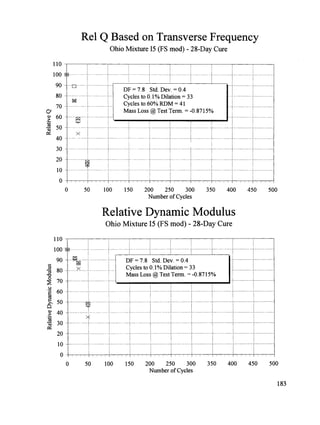
201. Mass Loss After Freezing and Thawing
Mixture MN1 - 28-Day Cure
2.5
2o : 0F=9 9
st oev--04
...............
1.5 Cycles to 0.1% Dilation = >>980 ...................................................................................
m 1.0 Cycles to 60% RDM = >>980 ................................
_
.................................................................
O
0.5 .......................................................................................................................................................................
_
..........................................................
i...................................
i...................................................................
-0.5 .............................................................................................................................................................................................
ID
-1.0 .............................................................................................................................................................................................
-1.5 ..............................
i....................................... i..............................
-2.0 ......................................................
i.................................
i. ii =, i
i
2 _ i
0 100 200 300 400 500 600 700 800 900 1000
Number of Cycles
Dilation after Freezing and Thawing
Mixture MN 1 - 28-Day Cure
o.25 i, i ,i i
0.20 ................................
i.............................................................................................................................
i...............................
i................................
i...................................................................................
oF=9 9
st oev:O4
!
Cycles to 60% RDM = >>980
= 0.15 ..........................................................................................................................
.2 Mass Loss @ 300 Cycles = 0.1001%
"_ i ==
0.10 ............................
............................
i..............................................................................................................................................................
tl)
o
0.05
...............................
i.......................
i
.......................
i
.................................
i.............................
i
................................
i
..................................
i
..................................
i
.................................
i
................................
i i i i i _& _i [] i i []
-0.05 _ _ _ I J _ _ : : ; I I _ _ _ I _ _ _ I _ _ _ I + _ I _ _ _ ! J :
0 100 200 300 400 500 600 700 800 900 1000
Number of Cycles
186

202. Rel Q Based on Transverse Frequency
Mixture MN1 - 28-Day Cure
110
loo+........................................................................
i
..........................................................
i
..................................
i
..............................
90 1 .........................................................................................
i...............................................
_ ....................
x:_ ..............................
i-_ ...................
i......................................................
A
80 .................
_.......z
..... _ _ .+ z. _. _ _ +
_1_+ i_;_i:_i_
__i _ _ _ _, " _ ............................
_i_
.................................
_ _
.................................
'................................
[]
O' 70 .........................................
_ .............
t........................................
_ ............
'..................
-'-t ...............................
_
..............................
i...........................
_
.................................
_
.................................
,u, 60 .......................................................
i...................................................................................
i..........................
}
.................................
E
..........................................................................
"_ 50
....................................................
i.........................
i................................................................
30 Cycles to 0.1% Dilation -- >>980
Cycies to 60% RDM = >>980
20 Mass Loss @ 300 Cycles = 0.1001%
10
0 _ _
0 100 200 300 400 500 600 700 800 900 1000
Number of Cycles
Relative Dynamic Modulus
Mixture MN1 - 28-Day Cure
110 i
, i _
100 __i_1__i____ ...........
i.................
_i .................
__ .......................
__ ...........................................................................
_
i
90 ..................................................................................................
_
.............................
i
_ ! i...........................................................
-u
"_ 80 ..............................................................................................................................................
"
.....................................................................................................................
o
70 ................................................................
DF = 98.9 Std. Dev. = 0.4 .......................................................................
"_ 60 ...................................................................
Cycles to 0.1% Dilation = >>980 .......................................................................
_, 50 .......................................................................
Mass L°ss @ 300 Cycles = 0 1001% .......................................................................
40 ............................................................................................................................................................................................
30 ............................................................................................................................................................................................
20 ............................................................................................................................................................................................
0 ..........................................................................................................................................................................................
:...................................................................................................................................
o , , , i ......... i_, , i ...... i ...... i , , ,
0 100 200 300 400 500 600 700 800 900 1000
Number of Cycles
187

203. Dilation after Freezing and Thawing
Mixture MN2 - 28-Day Cure
0.25 i i i i
0.20 ............................
i........................
i..............................
_
................................
i................................
_
..............................
i..............................
_
................................
_i.................................
_
..................................
i i DF -- 98.4 Std Dev = 0.6 I
Cycles to 60% RDM = >>980 |i
=o 0.15 ..........................................................
Mass Loss @ 300 Cycles = 0.1028% |i ................................................................
I
0.00 _ _ i"_ _ _i _ _ = _ _ _ i '_ i i i Y:
-0.05 ,,, i,,, i + ,, i ...... i ...... i,,, i,, , i , , ,
0 100 200 300 400 500 600 700 800 900 1000
Number of Cycles
Mass Loss After Freezing and Thawing
Mixture MN2 - 28-Day Cure
2.5
i!!-i iiiiii!-iii'iii i!
iiiii!!
!
!!!!!!!
i!!i!!
i
i
!!!
1.5 ]._...]
] Cycles to 0.1% Dilation = >>980
Cycles to 60% RDM = >>980
1.0
tJl
O i T I
o.o
-0.5 ...........................................................................................................................................................................................
__.o
.................................................................
il..........................
i il i ii i;
-1.5 ..........................
i......................
".........................
i
i-
] i i ..........
i
-2.0 ........................................................................................................ _
-2.5 ,, _ i _ , _ i , _, i _ _ , _ _ i i i
0 100 200 300 400 500 600 700 800 900 1000
Number of Cycles
188

204. Rel Q Based on Transverse Frequency
Mixture MN2 - 28-Day Cure
110 .
l []
100 ...........................
i ...................................
i.......................................................
i.................................................................
]
.................................
90 .......................
_.
................................
i................
_i .............
Q .............
i.................
_q .............
7__ ......................
D(-.._ ................
i.................................
F
.......................
_
70 .................................
} + ..............
i---+
..........................................
i................................
_
.........................
_
............................
b--+.................
i..............................
i......................
_..
O' []
o 60 .............................................................................................................................................................................................
•
-_ i i
40 .............................................................
i...: .......................................................................
DF = 98.4 Std. Dev. = 0.6
30 ...............................................................
Cycles to 0.1% Dilation = >>980 ......................................................................
20 .................................................................
Cycles to 60% RDM = >>980 ....................................................................
Mass Loss @ 300 Cycles = 0.1028%
10 ..............................................................
i.......... _
0 , i _ i _ _ _ _ _
0 100 200 300 400 500 600 700 800 900 1000
Number of Cycles
Relative Dynamic Modulus
Mixture MN2 - 28-Day Cure
110 i
90 ............................................................................................................................................................................................
•
_
80o DF=98"4 StdDev'=0"6 ......................................................................
70 Cycles to 0.1% Dilation = >>980 ......................................................................
._ Mass Loss @ 300 Cycles = 0.1028%
=_ 60 ......................................................................
;_ 50 .............................................................................................................................................................................................
o 40 .............................................................................................................................................................................................
20 .................................................................................................
_
...............................................................................................................................................
0 .....................................................................................................................................................................................................................................................................................................................................
0 100 200 300 400 500 600 700 800 900 1000
Number of Cycles
189

205. Dilation after Freezing and Thawing
Mixture MN3 - 28-Day Cure
0.25 i i i i
i ..........................................
0.20 ...........................................................
_
............................
i _ , ----_
DF = 97.6 Std. Dev. = 1.1
Cycles to 60% RDM = >>952 i
0.15
o Mass Loss @ 300 Cycles = 0.1185%
i
'=_ i
OO.lO
..........................
]
................................................
i
...............
0.05 ..............................................................................................
_
..................................
_ .ii
................................
i
0.00 _@iNNNiNNN N _ [] N@ •i _ i
-0.05 ............... I_:_ .....
0 100 200 300 400 500 600 700 800 900 1000
Number of Cycles
Mass Loss After Freezing and Thawing
Mixture MN3 - 28-Day Cure
2.5
2.0
i!iiii
iiii'
ii
iiii
iiiiiii
I° :9 6 y les
too v.:
l.loila on:
...........
1.5 • Cycles to 60% RDM = >>952 .........................................................................
1.0 ........................................................................
o i i i i
.a 0.5 .............................
i...............................
}
..........................................................................................................................
!
...............................................................
_.............
o
° -0.5 .............................................................................................................................................................................................
_
.................................................................................................
O
-1.0 .............................................................................................................................................................................................
-].5 ......................................................................................
_
...............................
_ ....................................
i_ ..........................................
i i i i
-2.0 .............................
i
k
i _ i i i
0 100 200 300 400 500 600 700 800 900 1000
Number of Cycles
190

206. Rel Q Based on Transverse Frequency
Mixture MN3 - 28-Day Cure
11o
lOO ...........................................................................................................................................................................
80 ....
_ ......................................
_-.---_
.............
_....-.-z
.............
_
..................
_---..-.J
................
®.....ta
......................
_......._
.....................
i []
70 .........................
i........................
i..........................
i...................................
_
.........................
i..........................
i...............................
i..................................
i...................................
i...........................
60 ! i i x
.............................................................................................
i.......................................................................................................................................
Z .....................................................................................
i
0 .......................................................... -......................................................................
DF = 97.6 Std. Dev. = 1.1
30 ..................................................................................................................................................
Cycles to 0.1% Dilation = >>952
20 ................................................................
Cycles to 60% RDM = >>952 ................................................................
10 .............................................................
Mass Loss @ 300 Cycles = 0.1185% ................................................................
i
0 i _ i i ' ' I
0 100 200 300 400 500 600 700 800 900 1000
Number of Cycles
Relative Dynamic Modulus
Mixture MN3 - 28-Day Cure
110
90 ......................................................................................................
i.......................................................................
i...........................................................
i..............................
_
..................................
_
.............
.x............
-_ 80 ......................................................................
DF=97.6 Std. Dev.=l.1 j
o
70 ...........................................................................
Cycles to 0.1% Dilation = >>952 ............................................
i_
..................................
60 ..........................................................................
Mass Loss @ 300 Cycles = 0.1185% ..........................................
!
..................................
_, 50 ..............................................................................................................................
*_ 40 ............................................................................................................................................................................
_
..................................
_.
.=_
30 ............................................................................................................................................................................
20 ............................................................................................................................................................................
0 ............................................................................................................................................................................................................................................................................................................................
0 , i ,[], i , , , i , , , i , , , i , , , i ,' , ,' , , , i , , ,
0 100 200 300 400 500 600 700 800 900 1000
Number of Cycles
191

207. Dilation after Freezing and Thawing
Mixture MN4 - 28-Day Cure
0.20 ....................................................................................................................
i.............................
i
..........................
i ..............................................
DF = 97.9 Std. Dev. = 0.3
= 0.15 ............................................................
Cycles to 60% RDM = >>980 ..................................................................
.2 Mass Loss @ 300 Cycles = 0.0989%
.,,m
0.10 .........................................................................................................................................................................................
Q_
_, o.o5 .............................................................
,............................
, i i
...........................
_
..........................................................................
J i
0.00 __,_; _; i _ i _ x z
i
i , i i
-0.05 .... _ _ : , _ : I, : _ , ' : , ' ,, _ : _ _ I : .
0 100 200 300 400 500 600 700 800 900 1000
Number of Cycles
Mass Loss After Freezing and Thawing
Mixture MN4 - 28-Day Cure
2.5 !
_ 1.0 "
0.5 ................................................................................................................................................................................
!
................................................................................................
-0.5 .......................................................................................................................................................
i...............................................................................................................
-1.0 .........................................................................................................................................................................
"
................................................................................
-2.0 ............................................
i
-2.5 _ _ i
0 100 200 300 400 500 600 700 800 900 1000
Number of Cycles
192

208. Rel Q Based on Transverse Frequency
Mixture MN4 - 28-Day Cure
110 _
_.. .... _ i i i
100 • _:
................... i..........................
_
........................
,..........................
_
............................
_- +! i E +
90 ..........
i...... + • i...........................................
-_...................................
i........................
i-.----+
...................
i.......................
i..............................
so_1_.i_ ix._ .x.!..._.-._
.._.....
B............
_
................
_.............
"_-
..............
_-.--.-._
...............
70 - i i } i 7. ................................................
_...
O'
60 ................................
_ ............
, ..................................................
i..........................................................................
'> i
50 ..................................................................................................................................................
_
.........................................................
¢_ [ DF = 97.9 Std. Dev. = 0.3
30 . ..... - Cycles to 60% RDM = >>980 .........................................................................
20 Mass Loss @ 300 Cycles = 0.0989% .......................................................................
10 .......................
:.
..............................................................
_ i i
i _ ! i i
0 100 200 300 400 500 600 700 800 900 1000
Number of Cycles
Relative Dynamic Modulus
Mixture MN4 - 28 Day Cure
110
100 _ _i__i_" I_ ___ ...........
i................
_ ......................
__ ...................
__ ....................................................................
i_
9o ........................................................................................
i ........................
i...............................
i..........................
i............................................................
" I: :
_ 80 DF=97.9 Std. Dev.=0.3
o Cycles to 0.1% Dilation = >>980
70 Mass Loss @ 300 Cycles = 0.0989% "
60 i
5o ...............................................................................................................................
._ 40 .............................................................................................................................................................................................
"_ 30 .............................................................................
i..................................................................................................................
i............................................................................
20 .......................................................................................
_
..................................................................................................................................
0 ...........................................................................................................................................................................................................................................................................................
0 : , , i , , i : , , i , , , i , , , i ...... i ...... i, , ,
0 100 200 300 400 500 600 700 800 900 1000
Number of Cycles
193

209. Dilation after Freezing and Thawing
Mixture MN5 - 28-Day Cure
0.25 i i i i
i i +
0.20 ...............................................................
+
...............................
+
..................................
+ .i
........................
+........ _ _
................................
+
DF = 92.5 Std. Dev. = 3.2 I
Cycles to 60% RDM = 582
._ 0.15 ..................
Mass Loss @ 300 Cyc. = 0.046% ................................
_ ...................................................................................
0.10 ...............................
i.......................................................................................................
+..4 .........................
[] .....................
_i...................................................................................
0.05 -!- []
+ m[] i
++++[][]+ []
0.00 _ [] _ ' _ ' +
+ i + i
+ + + i
i +
-0.05 + _ , , .... , + + _ , ...... I _ + + L _ , I _ +
0 100 200 300 400 500 600 700 800 900 1000
Number of Cycles
Mass Loss After Freezing and Thawing
Mixture MN5 - 28-Day Cure
2.5 i ;+ i +
..............................
I +:
586
[i!ii
iii!!
iii
ii
_ 1.0
O i................................
' ................................
'...............................
0.5 ...................................................................................................................
i-
ra i [] _i
i + .
............ + +
_
_ -0.5 ...................................................................................................................................................
i................................................................................................................
-1.5 .......................................................................................................................................................
"
...............................................
+
............................................................
-_.o
................................
+ ........
i + .........................................................
i
i i i i
-2.5 , , , , , , , , , , , , , + , , , + , + , +
0 100 200 300 400 500 600 700 800 900 1000
Number of Cycles
194

210. Rel Q Based on Transverse Frequency
Mixture MN5 - 28-Day Cure
110 _ i
100 ...........................................................
[ DF = 92.5 Std. Dev. = 3.2 ]
90 i_ Cycles to 0.1% Dilation = 586
%° t i
80 .......................
i..........................
,......................
_ ...............................
i.. Cycles to 60% RDM = 582
_c3[] oi i i Mass Loss @ 300 Cycles = 0.046%
70 ...............................
_--_ ........
_--_
......................
_
............................
i.,
+i+ _ _D i_
CY _ i
60 .......................................
+........................
+....-..!
............
[]............
i................................................................................................................................
-_ 5o
40 ..........................
i...............................................................................................................................................................
i...............................
i............................................................................
20 ..................................................................................................................................................................................
[]............................
i..................................................................................
O .............................................................................................................................................................................................................................................................................................................
0 1O0 200 300 400 500 600 700 800 900 1000
Number of Cycles
Relative Dynamic Modulus
Mixture MN5 - 28-Day Cure
llO i i
_oo_._ i®_i__ _ _...................................................................
90 ...........................
_.............................
i...........................
_......._.............
i..................
[] .4...............................
i...............................
_
...................................
_
.................................
_
..................................
•
a 80 ......................................................................................................................
_
.............................................................
i
.............................................................
o [] i
70 ...................................................................................................................................
+ "i
_
...............
®_ ................................................................................................
'_ 60 ..........................................................................................................................................................
i..........................
_ ................................................................................................
50 ............................
i............................................................................................
i...........................
i.................
T ...................................
[] ...................................................................................
i21 i i
•' 40 ............................
i............................................................
i...............................
i i
--_ 30 ] - DF= 92.5 Std. Dev. = 3.2 .......................................................................................................
Cycles to 0.1% Dilation = 586
20 I Mass Loss @ 300 Cycles = 0.046% .......................................................................................................
10 _ i ..........
i.....................................................................
i
..................................
i
..................................
0 100 200 300 400 500 600 700 800 900 1000
Number of Cycles
195

211. Dilation after Freezing and Thawing
Mixture MN6 - 28-Day Cure
0.25 i i i
i i
0.20 ....................................................
_
.............................._ _i ............
_ _ .........................................
DF = 99.2 Std. Dev. = 0.5 ] +
Cycles to 60% RDM = >>980
I
= 0.15 ........................................................... .....
o Mass Loss @ 300 Cycles = 0.1054%
.=_
•
"= i i
0.10
t_
0.05 ...........................
_
.......................................................
i..............................
, .................................................................
.+_
0.00
_T-I q- i+ H- +i -_-
-[-. -4- + i -_- _-
i i ! i
0 100 200 300 400 500 600 700 800 900 1000
Number of Cycles
Mass Loss After Freezing and Thawing
Mixture MN6 - 28-Day Cure
2.5 _
i i '
2.0 .........................................................................................................................................
i..........................
i. i .............................................................
I DF = 99.2 Std. Dev. = 0.5
151..i CYclest° 0 1%Dilafi°n = >>980 .........................................................................
1.0 = Cycles to 60% RDM = >>980 ........................................................................
_ 0.5 ...............................................................................................
L
...............................................................................................................................
_ 0.5 ..........................................................................
_
...............................................................................................................................................
-1.0 ............................................................................................................................................................................................
-2.0 ............................................................................................................................................................................................
0 100 200 300 400 500 600 700 800 900 1000
Number of Cycles
196

212. Rel Q Based on Transverse Frequency
Mixture MN6 - 28-Day Cure
110 j
x _ x
100 ............ _
...................
_
..................... E
.......................................................
_...........................
_ .................
x +_ xi, [] []
90 ......................
[] .........
_
...............................
_
..........................
_
..................................
El....+
.....................
_i...................................................................................
: ........................ ...........................
i ...............................
i........................
_i ..........................................................................................
80 .@.._ -..+-_ _ +
70 ............... _
...................
I i .............................................................................
O_
o 60 ............................................................................................................................................................................................
•-_ i
-_ 50 ..............
,................................................
_
................................................................................................................................................
40
i!it st' ev:°
30 Cycles to 0.1% Dilation = >>980
Cycles to 60% RDM = >>980
20 Mass Loss @ 300 Cycles = 0.1054%
10 .... .
i i _ i i
0 100 200 300 400 500 600 700 800 900 1000
Number of Cycles
Relative Dynamic Modulus
Mixture MN6 - 28-Day Cure
110 _ _ i
_oo_.®. _®_-i--®-_---®.....®
.......
i
.................
_---i
............
_.-_
....................
_i..._
.............................................
_..
i i '
90 .................................................................................................
i
......................................................
i
..................................................................
_ 80 .....................................................
DF=99.2 Std. Dev.=0.5
o Cycles to 0.1% Dilation = >>980
.-E 70 ..................................................................
Mass Loss @ 300 Cycles = 0.1054% . "
60 .............................................................
5o ..............................................................................................................................
40
"_ 30 .....................................................
i...............................................................................................................................................................
20 .......................................................
i...............................................................................................................................................................
0 ...............................................................................................................................................................................................................................................................................................
0 100 200 300 400 500 600 700 800 900 1000
Number of Cycles
197

213. Dilation after Freezing and Thawing
Mixture MN7 - 28-Day Cure
0.25 i i i i i i []_
..................
DF = 91.4 Std. Dev. = 6.5 I
0.20 Cycles to 60% RDM = 663 ................................................................................................
Mass Loss @ 300 Cycles = 0.0731%
I
,. 0.15 ..........................
i..................................................................
_
.................................. i..................................................................................................
o _ xi
i i i i
o.o5 .................................
i
..........................................................................................................................
i _ ....................................
i i _ i +i i
0.00 i .... i
-0.05 _ _, , ..... , ........ ' _ _ ' ' ' _ '
0 100 200 300 400 500 600 700 800 900 1000
Number of Cycles
Mass Loss After Freezing and Thawing
Mixture MN7 - 28-Day Cure
2.5 i i , _
!i
i!i
!ii!!!i
!ii!!.
!
i!
!i
!!
iDF:
9,.4
Oev.
:
Cy les
Cy ,es
to
,oD , ion
663:
649
iIi!!!
i !
_ 1.0 '
_ i i i i i +
0.5
o.o
-0.5 ............................................................................................................................................................................................
-1.0 .............................................................................................................................................
ii
0 100 200 300 400 500 600 700 800 900 1000
Number of Cycles
198

214. Rel Q Based on Transverse Frequency
Mixture MN7 - 28-Day Cure
100 DF = 91.4 Std. Dev. = 6.5
90 Cycles to 0.1% Dilation = 649
![] i + i i i Cycles to 60% RDM = 663
80 _-_
..... [].....i_..ix
_z.............
[]ii..................................
_!
.............................
i..i
-1 Mass Loss @ 300 Cycles = 0.0731%
......
_................
i+...............
-_ .-i..-.._..-.-_
.....................
_-.................
t
60 .........................................................................................
'_
...............................
i................................................................................................................................
•B X _ [] +
¢_ x i i
i i
40 .....................................................................
.Z..................................
[]...........................................................
_i .......................
+ .....................................................................
30 ............................................................................................
i...........
N...........................................................................................................
i.............................
"+........................................................
N
20 ..............................................................................................................................
_' -®.....................
Ni..................................................................................
+.
0 ..........................................................................................................................................................................................................
i........................................................................................................................
0 100 200 300 400 500 600 700 800 900 1000
Number of Cycles
Relative Dynamic Modulus
Mixture MN7 - 28-Day Cure
110 i
lOO_._.. ___i__U_ ....................................................................................
i................................
i
...............................
90 .................................
_
............................
_
...............................................
_' ............
_
............................................
+..----.-._
...................................
i..................................................................
_
...................................
m N i i + ! i i
-_ 8o ..............................
,.............................
_ s _-.i..............................
i
...........................
±i
...............................
i...............................
i
................................
o [ .......................................................................
i.+ .......................
i.................................
70 ................................ i
"_ "
...................................................................................................................................................
_ ...........................................................................................................
i..................................
I.........................
_
_ 60 i i ! _ i i ! i
50 .........................................................................................................................
_ ...............................................................
Cl @
40 .................................
i......................
i.................................
i...............................
i...................................................................................................................
._,_
__ DF = 91.4 Std. Dev. = 6.5
30 Cycles to 0.1% Dilation = 649 ................................................................................................
[]i
20 Mass Loss @ 300 Cycles = 0.0731% .................................................................................................
0 .............................................................................................................................................................................................................................................................................................................................................
0 ,,, i,, ,i,,,i ......... i,,,', ...... i, ,,
0 100 200 300 400 500 600 700 800 900 1000
Number of Cycles
199

215. Dilation after Freezing and Thawing
Mixture MN8 - 28-Day Cure
0.25 i
0.20 ......................................................................
DF = 98.4 Std.Dev. = 0.3
i Cycles to 60% RDM = >>980
=o 0.15 .........................
_i
.............................
Mass Loss @ 300 Cycles = 0.0467% .....................................................................
•-" !
0.10 ...................................................................................................................................................................
_
...................................................................................................
o 1
¢_ 0.05 ............................................... B........I. _.
2K
o.oo_i_-= _ _ _ _i []
L i ,
0 100 200 300 400 500 600 700 800 900 1000
Number of Cycles
Mass Loss After Freezing and Thawing
Mixture MN8 - 28-Day Cure
2.5 _
i
2.0 .............................................................................................................................................
DF = 98.4 Std.Dev. = 0.3
1.5 ...................................................................
Cycles to 0.1% Dilation = >>980 ............................................................................
Cycles to 60% RDM = >>980 []
).0 .......................................................................................................................................................
o i i
0.5 ...................................................................................................................................................................
i...............................
i.........................
, i....................
>_.
-0.5 .................................................................................................................................................
O
-2.0 ..........................
_ ..................................................................
•
,...............................
[ i......................
i .i
-2.5 , , , _ _ _
0 100 200 300 400 500 600 700 800 900 1000
Number of Cycles
200

216. Rel Q Based on Transverse Frequency
Mixture MN8 - 28-Day Cure
lOOi ...................
i.......................
i.........................................................................................
×._..i
....................
i +.
80 "z: .................................................................................................................................................................................
Lx[] x i x
70 ........................................................ ,.........................
_ _
50 ...........................
_
...........................
_
..........................
0 ........................................................................................................................................
DF = 98.4 Std. Dev. = 0.3
30 ......................................................
Cycles to 0.1% Dilation = >>980 .....................................................................
20 ......................................................................
Cycles to 60% RDM = >>980
Mass Loss @ 300 Cycles = 0.0467%
10 ...............................................
_
............................................. i..........................
o i i i i i _ _*
0 100 200 300 400 500 600 700 800 900 1000
Number of Cycles
Relative Dynamic Modulus
Mixture MN8 - 28-Day Cure
110
100 _-_IEN_[]i-Z _Ii_--IN ...........
i.............
_i ..............
__ ............
_i-_ .................................................................
_
I
90 .....................................................................................
i........................................................................................................................
80 ...........................................................
DF = 98.4 Std. Dev. = 0.3
o Cycles to 0.1% Dilation = >>980
:_ 70 ...............................................................
.o MassLoss@ 300Cycles= 0.0467%
60 ..........................................................
_. 5o ........................................................................................................................................
o 40 ........................................................................................................................................
'........................
'
>
N
30 ...........................................................................................................................................................................................
20 ............................................................................................................................................................................................
10 ......................
ii i i ............................. i, ii
0 _ _ I _ I ' _ _ _ I _ I _ I _ : I _ _ _ I _ I
0 100 200 300 400 500 600 700 800 900 1000
Number of Cycles
201

217. Concrete and Structures Advisory Committee
James J. Murphy, chairman Liaisons
New York Department of Transportation (retired)
Theodore R. Ferragut
Howard H. Newlon, Jr., vice chairman Federal Highway Administration
Virginia Transportation Research Council (retired)
Crawford F. Jencks
Charles J. Arnold Transportation Research Board
Michigan Department of Transportation
Bryant Mat.her
Donald E. Beuerlein USAE Waterways Experiment Station
Koss Construction Co.
Thomas J. Pasko, Jr.
Bernard C. Brown Federal Highway Administration
Iowa Department of Transportation
John L. Rice
Richard D. Gaynor Federal Aviation Administration
National Aggregates Association Ready Mixed Concrete
Association Suneel Vanikar
Federal Highway Administration
Robert J. Girard
Missouri Highway and Transportation Department Expert Task Group
David L. Gress Paul Klieger, chairman
University of New Hampshire Consultant
Gary Lee Hoffman Stephen Forster
Pennsylvania Department of Transportation Federal Highway Administration
Brian B. Hope James G. Gehler
Queens University Illinois Department of Transportation
Carl E. Locke, Jr. Vernon J. Marks
University of Kansas Iowa Department of Transportation
Clellon L. Loveall Bryant Mather
Tennessee Department of Transportation USAE Waterways Experiment Station
David G. Manning Richard Meininger
Ontario Ministry of Transportation National Aggregates Association/
National Ready Mix Concrete Association
Robert G. Packard
Portland Cement Association Larry R. Roberts
W.R. Grace and Company
James E. Roberts
California Department of Transportation James H. Stokes
New Mexico State Highway Department
John M. Scanlon, Jr.
Wiss Janney Elstner Associates James Woodstrom
Consultant
Charles F. Scholer
Purdue University
Lawrence L. Smith
Florida Department of Transportation
John R. Strada
Washington Department of Transportation (retired)