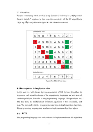
This dissertation presents the 'Square Root Sorting Algorithm' developed by Mir Omranudin Abhar under the supervision of Ms. Nisha Gautam as part of his Master of Technology in Computer Science and Engineering at APG Shimla University. It introduces a new sorting method that demonstrates improved time and space complexity compared to existing algorithms, particularly suited for large lists. The work is original and fulfills university requirements, with proper acknowledgment of guidance and support throughout the research process.


![1
CHAPTER 1
Introduction
This part describes an overview of whole this thesis which provides an
overarching theme of this thesis to reader.
1.1 Introduction
In the field of Computers, data management is the most crucial job. So, we need a
field that helps us in managing data which is known as data structure, A data
structure is a data organization, management and storage format that enables
effective access and modification [2]. In other words, Data structure is a
collection of data values, the relationships among them, and the functions or
operations that can be applied to the data [24].
Various operations are deploying in data structure:
1. Insertion: Insertion means addition of a new data component in a data
structure.
2. Deletion: Deletion means removal of a data component from a data
structure if it is found.
3. Searching: Searching includes searching for the specified data component
in a data structure.
4. Traversal: Traversal of a data structure means processing all the data
components present in it.
5. Sorting: Arranging data components of a data structure in a specified order
is called sorting.
6. Merging: Combining elements of two similar data structures to form a new
data structure of the same type, is called merging. [42]
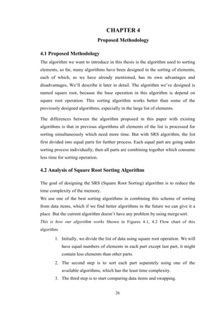
Sorting is one of the most important and valuable parts in the data structure,
Sorting is nothing but arrangement of a set of data in some order or a process
that rearranges the records in a file into a sequence that is sorted on any key
shown in figure 1.1 sorting algorithm. Different methods are used to sort the data
in ascending or descending orders. The different sorting methods can be
divided into two categories. They are
Internal sorting: We can define internal sorting as a sorting of data items in
the main memory.](https://image.slidesharecdn.com/srs-170016511-190723185008/85/Square-Root-Sorting-Algorithm-12-320.jpg)
![2
External sorting: External sorting is defined as a sorting when the data to be
sorted is so large that some of the data is present in the memory and some
is kept in auxiliary memory.
Arrays (sets of items of the same type of stored in contiguous memory space) are
stored in the fast, high-speed random access internal store on computers, whereas
files are stored on the slower but more spacious External store. [11]. the algorithm
that we introduce in this thesis is related to internal sorting algorithm. Some
common internal sorting algorithms include: Bubble Sort, Insertion Sort, Quick
Sort, Heap Sort, Radix Sort, Selection Sort, etc. Every sorting algorithm has some
advantages and disadvantages. The “Performance Analysis of Sorting
Algorithms” deals with the most commonly used internal sorting algorithms and
evaluates their performance. To sort a list of components, First of all we analyzed
the given problem i.e. the given problem is of which type (small numbers, large
values). The time complexity may vary depending on the sorting algorithm used.
Each sorting algorithm follows a unique method to sort an array of numbers either
by ascending or descending order [42].
The complexity of an algorithm is a function f (n) which measures the time and
space use by an algorithm in terms of input size n, in computer science, the
complexity of an algorithm is a way to classify how effective an algorithm is. As
compared to alternative ones. The emphasis is on how execution time increases
with the data set to be processed. The computational complexity and efficient
implementation of the algorithm are important in computing, and this depends on
suitable data structures [40].](https://image.slidesharecdn.com/srs-170016511-190723185008/85/Square-Root-Sorting-Algorithm-13-320.jpg)
![3
1.2 Data Structure and Algorithm
1.2.1 Data Structure
In computer science, with the help of an appropriate data structure the computer
system will perform its task more efficiently because the data structure
influencing the ability of the computer to store and retrieve data from any location
in its memory, A data structure is an individual way of storing and organizing data
in a computer so that it can be used efficiently. Different kinds of data structures
are suited to different kind of applications, and some arc highly specialized to
specific tasks, Data structures are used in almost every program or software
system. Data structures provides a means to manage huge amounts of data
efficiently, such as large databases and internet indexing services. Usually,
effective data structures are a key to designing efficient algorithms, some official
design methods and programming languages emphasize data structures, rather
than algorithms, as the key organizing factor in software design [13, 12].
Data structure deals with the study of how data is organized in the computer’s
main memory and how it maintains logical relationship between individual
elements of data and also, how efficiently the data can be retrieved and
manipulated. A data structure is a study of organizing all the data elements that
consider not only the elements stored but also their relationship with each other.
Data structures are the building blocks of a program and hence, the selection of a
particular data structure addresses the following two things. [7]
Data structures are generally based on the ability of a computer to fetch and
store data at any place in its memory, specified by an address - a bit string that can
be itself store in memory and manipulated by the program thus the record and
array data structures are based on computing the addresses of data items with
arithmetic operations, while the linked data structures are based on storing
addresses of data items within the structure itself, Many data structures use both
principles, sometimes combined in non-trivial ways. The implementation of a data
structure usually needs writing a set of procedures that create and manipulate
instances of that structure. The effective of a data structures cannot be analyze
separately from those operations, this observations motivates the theoretical
concept of an abstract data type a data structure that is defined indirectly by the
operations that may be performed on it, and the mathematical properties of](https://image.slidesharecdn.com/srs-170016511-190723185008/85/Square-Root-Sorting-Algorithm-14-320.jpg)
![4
those operations (including their space and time cost) [13].
• Data structure should be rich enough in structure for reflecting real
relationship existing between data.
• A structure must be simple such that we can process data effectively
whenever needed.
Classification: Data structure is broadly classified into two categories shown in
figure 1.2 categories of data structures.
1. Primitive data structures
2. Non-primitive data structures
1.2.1.1 Primitive data structures
These data structures are basic structures and are manipulated/ operated directly
by machine instructions. We will present storage representations for these data
structures for a variety of machines. The integer’s floating-point numbers (real
numbers), character constants, string constants, pointers etc. Are some of the
primitive data structures? In C language, these primitive data structures are
defined using data types such as int, float char and double. But you are already
aware of these representations in computer main memory [7].
1.2.1.2 Non-Primitive data structures
These data structures are more sophisticated and are derived from the primitive
structures. But, these cannot be manipulated/operated directly by machine](https://image.slidesharecdn.com/srs-170016511-190723185008/85/Square-Root-Sorting-Algorithm-15-320.jpg)
![5
instructions. A non-primitive data structure emphasize on structuring of a set of
homogeneous (same data type) or heterogeneous (different data types) data
elements. Arrays, structures, stacks queues linked lists, files etc. are some of the
non-primitive data structures [7].
1.2.2 Relation between Data Structure and Algorithm
Implementation of data structures can be done with the help of programs. To write
any program we need an algorithm. Algorithm is nothing but collection of
instructions which has to be executed in step by step manner. And data structure
tells us the way to organize the data. Algorithm and data structure together give
the implementation of data structures. To write any program we have to select
proper algorithm and the data structure. If we choose improper data structure then
the algorithm cannot work effectively. Similarly if we choose improper algorithm
then we cannot utilize the data structure effectively. Thus there is a strong
relationship between data structure and algorithm. As data structure can be very
well understood with the help of a programminglanguage [2].
Data Structure + Algorithm = Programs
1.2.3 Algorithm
Algorithm is a procedure or formula for solving a problem. The word derives
from the name of the mathematician, Mohammed ibn-Musa al-Khwarizmi, who
was part of the royal court in Baghdad and who lived from about 780 to 850. Al-
Khwarizmi’s work is the likely source for the word algebra as well [14, 18].
An algorithm is a step by step method of solving a problem [16]. It is commonly
used for data processing, calculation and other related computer and mathematical
operations [4]. Once an algorithm is given for a problem and decided to be
correct, an important step is to determine how much resources, in term of time or](https://image.slidesharecdn.com/srs-170016511-190723185008/85/Square-Root-Sorting-Algorithm-16-320.jpg)
![6
space, the algorithm will require. An algorithm that solves a problem but
requires a year is hardly of any use shown in figure 1.3 representation Algorithm
[41].
1.2.4 Implementation of Algorithm
To develop any program we should first select a proper data structure, and then we
should develop an algorithm for implementing the given problem with the help of
a data structure which we have chosen. Before actual implementation of the
program, designing a program is very important step. Suppose, if we want to build
a house then we do not directly start constructing the house. In fact we consult an
architect, we put our ideas and suggestions, accordingly he draws a plan of the
house, and he discusses it with us. If we have some suggestion, the architect notes
it down and makes the necessary changes accordingly in the plan. This process
continues till we are satisfied. Finally the blue print of house gets ready. Once
design process is over actual construction activity starts. Now it becomes very
easy and systematic for construction of desired house. In this example, you will
find that all designing is just a paper work and at that instance if we want some
changes to be done then those can be easily carried out on the paper. After a
satisfactory design the construction activities start. Same is a program
development process.
If we could follow same kind of approach while developing the program then we
can call it as Software development life cycle which involves several steps as -
a. Feasibility study
b. Requirement analysis and problem specification
c. Design
d. Coding
e. Debugging
f. Testing and
g. Maintenance
1.2.5 Analysis of Algorithm
Analysis of algorithm means to determine the amount of resources (such as time
and storage) required to execute it, most algorithms are designed to works with
inputs of arbitrary length. Usually the efficiency or current time of an algorithm is](https://image.slidesharecdn.com/srs-170016511-190723185008/85/Square-Root-Sorting-Algorithm-17-320.jpg)
![7
stated as a function relating the input length to the number of steps (time
complexity) or storage locations (space complexity) [10, 22].
Algorithm analysis is an important part of a widespread computational
complexity theory, which provides theoretical estimates for the resources needed
by any algorithm which solves a given computational problem. These estimates
provide an insight into reasonable directions of search for effective algorithms. In
theoretical analysis of algorithm it is common to evaluate their complexity in the
asymptotic sense, i.e., to estimate the complexity function for arbitrarily large
input [10, 6].
1.2.6 Analysis of Program
The analysis of the program does not mean simply working of the program but to
check whether for all possible situations program works or not. The analysis also
involves working of the program efficiently. Efficiency, means
• The program requires less amount of storage space.
• The program get executed in very less amount of time.
The time and space are the factors which determine the efficiency of the program.
Time required for execution of the program cannot be computed in terms of
seconds because of the following factors -
The hardware of the machine.
The amount of time required by each machine instruction.
The amount of time required by the compilers to execute the
instruction.
The instruction set.
Hence we will assume that time required by the program to execute means the
total number of times the statements get executed. This is known as frequency
count [2].
1.2.7 Complexity of Algorithm
The complexity of an algorithm is a function f (n) which measures the time and
space use by an algorithm in terms of input size n, in computer science, the
complexity of an algorithm is a way to classify how efficient an algorithm is,
compared to alternative ones, the emphasize is on how execution time
increases with the data set to be processed.](https://image.slidesharecdn.com/srs-170016511-190723185008/85/Square-Root-Sorting-Algorithm-18-320.jpg)
![8
The computational complexity and efficient implementation of the algorithm are
important in computing, and this depends on suitable data structures [29, 3]
If we have two algorithms that perform same task, and the first one has a
computing time of O (n) and the second of O(n2), then we will usually prefer the
first one. The reason is that as n increases the time required for the execution of
second algorithm is far more than the time required for the execution of first. We
will study various values for computing function for the constant values. The
graph given below will indicate the rate of growth of common computing time
functions [2] shown in figure 1.4 Rate of growth of common computing time
function.
Notice how the times O (n) and O (n log n) grow much more slowly than the
others, for large data sets algorithms with a complexity greater than O (n log n)
are often impractical. The very slow algorithm will be the one who is having the
time complexity as 2n [2] shown in table 1.1 Rate of growth of common
computing time function.
𝒏 𝐥𝐨𝐠 𝟐 𝒏 𝒏 𝐥𝐨𝐠 𝟐 𝒏 𝒏 𝟐
𝒏 𝟑
𝟐 𝒏
1 0 0 1 1 2
2 1 9 4 8 4
3 2 8 16 64 16
8 3 24 64 512 256
16 4 64 256 4096 65536
32 5 160 1024 32768 2147483648
1.2.7.1 Asymptotic Notation
Asymptotic notation describes the behavior of the time or space complexity for
large instance characteristics [21]. To select the best algorithm, we need to check
Table 1.1: Rate of growth of common computing time function](https://image.slidesharecdn.com/srs-170016511-190723185008/85/Square-Root-Sorting-Algorithm-19-320.jpg)
![9
efficiency of each algorithm. The efficiency can be measured by calculating time
complexity of each algorithm, asymptotic notation is a shorthand way to represent
the time complexity. Use asymptotic notations we can give time complexity as
“fastest possible”, “slowest possible” or “average time”. Various notations such as
Ω, θ and O used are called asymptotic notions [1].
1.2.7.1.1 Theta Notation : Theta notation denoted as ’θ’ is a method of
representing running time between upper bound and lower bound.
Explanation: Let, f (n) and g (n) be two non-negative functions. There exists a
positive constant C1 and C2 such that C1g (n) ≤ f (n) ≤ C2g (n) and f (n) is theta
of g of n [1, 2] shown in figure1.5 Figure Asymptotic Notation (a).
1.2.7.1.2 Big Oh Notation: Big Oh notation means by ’O’ is a method of
representing the upper bound of algorithm’s running time. Using large oh notation
we can give longest amount of time taken by the algorithm to complete.
Explanation: Let, f (n) and g (n) are two non-negative functions. And if there
exists an integer no. and constant C such that C > 0 and for all integers n > n0, f
(n) ≤ c ∗ g(n) , then f (n) is big oh of g(n). It is also denoted as “f (n) = O (g (n))”
[1,2] shown in figure1.5 Asymptotic Notation (b).
1.2.7.1.3 Omega Notation: Omega notation denoted as Ω is a method of
representing the lower bound of algorithm’s running time. Using omega notation
we canmeansshortest amount of time taken by algorithm to complete.
Explanation: Let, f (n) and g(n) are two non-negative functions and if there exists
constant C and integer no. such that C > 0 and n > no then f (n) > C ∗ g(n) i.e.
f(n) is omega of g of n. This is denoted as f (n) = Ω (g (n))[1, 2] shown in figure1.5
Asymptotic Notation (c).
(a) : Theta Notation (b) : Big O Notation (c) : Omega Notation](https://image.slidesharecdn.com/srs-170016511-190723185008/85/Square-Root-Sorting-Algorithm-20-320.jpg)
![10
1.2.7.2 Space Complexity
Another useful measure of an algorithm is the amount of storage space it needs.
The space complexity of an algorithm can be computed by considering the data
and their sizes. Again we are concerned with those data items which demand for
maximum storage space. A similar notation ’O’ is used to denote the space
complexity of an algorithm. When computing for storage requirement we assume
each data element needs one unit of storage space. While as the aggregate data
items such as arrays will need n units of storage space n is the number of
elements in an array. This assumption again is independent of the machines on
which the algorithms are to be executed [2].
To calculate the space complexity we use two factors: constant and instance
characteristics, the space requirement S (p) can be set as
S(p) = C + Sp
Where C is a constant i.e. fixed part and it mean the space of inputs and outputs,
this space is an amount of space taken by instruction, variables and identifiers.
Sp is a space dependent upon instance characteristics. This is a variable part
whose space requirement depends on particular problem instance [1].
Constant Complexity: O (1)
A constant tasks run time won’t change no matter what the input value is,
considera function that prints a value in an array.
No matter which components value you’re asking the function to print, only
one step is required. So we can say the function runs in O (1) time; its run-time
does not increase. Its order of magnitude is always 1[19, 5].
Linear Complexity: O (n)
A linear tasks run time will vary depending on its input value, if you ask a function to
print all the items in a 10- component array, it will require less steps to complete than it
would a 10,000 element array. This is said to run at O (n); its run time increases at an
order of magnitude proportional to n [19, 5].](https://image.slidesharecdn.com/srs-170016511-190723185008/85/Square-Root-Sorting-Algorithm-21-320.jpg)
![11
Quadratic Complexity: O (N 2)
A quadratic task requires a number of steps equal to the square of its input value.
Let’s look at a function that takes an array and N as its input values where N is
the number of values in the array. If I use a nested loop both of which use N as its
limit condition, and I ask the function to print the arrays contents, the function
will perform N rounds, each round printing N lines for a total of O (N 2) print
steps. Let’s look at that practically. Assume the index length N of an array is 10,
if the function prints the contents of its array in a nested-loop, it will perform 10
rounds, each round printing 10 lines for a total of 100 print steps. This is said to
run in O (N 2) time; its total run time increases at an order of magnitude
proportional to 𝑁2
[19, 5].
Exponential: O (2n)
O (2n) is just one example of exponential growth (among O (3n), O (4n), etc.).
Time complexity at an exponential rate means that with each step the function
performs, its subsequent step will take longer by an order of magnitude
equivalent to a factor of N, For instance, with a function whose step-time doubles
with each sub sequent step, it is said to have a complexity of O (2n). A function
whose step-time triples with each iteration is said to have a complexity of O (3n)
and so on [19, 5].
Logarithmic Complexity: O (log n)
This is the type of algorithm that makes calculation blazingly fast, Instead of in-
creasing the time it takes to perform each subsequent step, the time is decreased at
magnitude inversely proportional to N.](https://image.slidesharecdn.com/srs-170016511-190723185008/85/Square-Root-Sorting-Algorithm-22-320.jpg)
![12
Let’s say we want to search a database for a particular number. In the data set
follow, we want to search 20 numbers for the number 100, in this example,
searching by this 20 numbers is a non-issue. But imagine were dealing with data
sets that store millions of users profile information, searching through each index
value from starting to end would be ridiculously inefficient. Especially if it had to
be done multiple times.
A logarithmic algorithm that performs a binary search looks through only half of
an increasingly smaller data set per step, assume we have an ascending ordered set
of numbers. The algorithm starts by searching half of the entire data set. If it
doesn’t find the number, it discards the set just checked and then searches half of
the remaining set of numbers.
Round printing 10 lines for a total of 100 print steps. This is said to run in O (N 2)
time; its total run time increases at an order of magnitude proportional to N 2.
As illustrated above, each round of searching consists of a smaller data set than
the previous, decreasing the time each subsequent round is performed. This makes
log n algorithms very scalable [19, 5].
1.3 Sorting Algorithm
Introduction-In the previous section, we described the Data Structure, Algorithm,
Complexity, and the relation between the data structure and Algorithm.
Examined the complexity of the algorithm.](https://image.slidesharecdn.com/srs-170016511-190723185008/85/Square-Root-Sorting-Algorithm-23-320.jpg)
![13
In this section we will discuss about existing sorting algorithms and examining
their complexities.
1.3.1 Sorting
Sorting is any process of organizing items in some sequence and/or in different
sets, and accordingly, it has two common, yet distinct meanings:
• Ordering: organizing items of the same kind, class, nature, etc. in some
ordered sequence,
• Categorizing: grouping and labeling items with equivalent properties
together (by sorts).
In computer science, a sorting algorithm is an algorithm that puts components of a
list in a some order, the most-used order are numerical order and lexicographical
order, beneficial sorting is important for improve the use of other algorithms
(such as search and merge algorithms) that require sorted lists to work correctly; it
is also often useful for cannibalizing data and for producing human-readable
output 20] shown in figure 1.6 Sorting Algorithm.
Every sorting algorithm has some advantages and disadvantages, the
“Performance analysis of sorting algorithms” deals and analyze the most generally
used internal sorting algorithms and evaluate their performance. To sort a list of
components, First of all we analyzed the given problem i.e. the assumed problem
is of which type (small numbers, large values). The time complexity may vary
depended upon the sorting algorithm used, each sorting algorithm follows a
unique method to sort an array of numbers either by ascending or descending
order [42].
Many computer scientists discuss sorting to be the most fundamental problem in
the study of algorithms. There are several reasons [43]:
1. Sometimes an application inherently requirements to sort information. For
example, in order to prepare client statements, banks need to sort checks by
check number.
2. Algorithms often use sorting as a key sub routine. For example, a program
that render graphical objects that are layer on top of each other might have
to sort the objects according to an ”above” relation so that it can draw](https://image.slidesharecdn.com/srs-170016511-190723185008/85/Square-Root-Sorting-Algorithm-24-320.jpg)
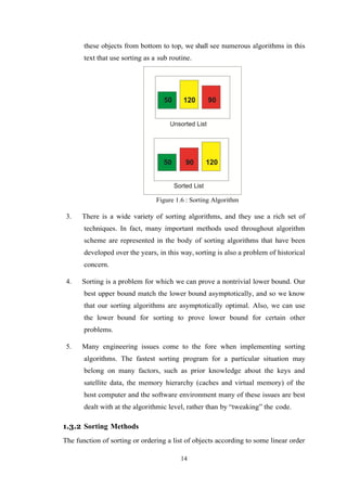
![15
is so fundamental that it is ubiquitous in engineering applications in all
disciplines. There are two broad categories of sorting methods [25]:
1. Internal sorting takes place in the main memory, where we can take
advantage of the random access nature of the main memory;
Quick Sort
Heap Sort
Bubble Sort
Insertion Sort
Selection Sort
Shell Sort and etc.
2. External sorting is necessary when the number and size of objects are
prohibitive to be accommodated in the main memory
Merge Sort
Radix Sort
Polyphase Sort and etc.
1.3.2.1 Bubble Sort
Bubble Sort is a simple algorithm which is used to sort a given set of n components
provided in form of an array with n number of components. Bubble Sort
compares all the elements one by one and sort them based on their values. If the
given array has to be sorted in ascending order, then bubble sort will start by
matching the first element of the array with the second element, if the first
element is greater than the second component, it will swap both the elements,
and then move on to compare the second and the third element, and so on. If we
have total n components, then we need to repeat this process for n-1 times.
It is known as bubble sort, because with every complete iteration the largest
component in the given array, bubbles up towards the last place or the highest
index, just like a water bubble rises up to the water surface. Sorting takes place
by stepping through all the elements one-by-one and matching it with the
adjacent component and swapping them if required.
Following are the Time and Space complexity for the Bubble Sort algorithm [8].](https://image.slidesharecdn.com/srs-170016511-190723185008/85/Square-Root-Sorting-Algorithm-26-320.jpg)
![16
Table 1.2: Bubble Sort
Worst Case Average Case Best Case
Time Complexity n2 n2
n
Space Complexity 1 1 1
1.3.2.2 Insertion Sort
Insertion sort is based on the idea that one component from the inputs components
is consumed in each iteration to find its correct position i.e., the position to which
it belongs in a sorted array.
It iterates the input components by growing the sorted array at each iteration. It
compares the current component with the largest value in the sorted array. If
the current element is greater, then it leaves the element in its place and moves
on to the next component else it finds its correct position in the sorted array and
moves it to that position. This is done by shifting all the components, which are
larger than the current element, in the sorted array to one position ahead [15].
Following are the Time and Space complexity for the Insertion Sort algorithm [8].
Worst Case Average Case Best Case
Time Complexity n2 n2
n
Space Complexity 1 1 1
1.3.2.3 Selection Sort
Selection sort is conceptually the easy sorting algorithm. This algorithm will first
find the smallest component in the array and swap it with the component in the
first position, then it will find the second smallest component and swap it with the
component in the second position, and it will keep on doing this until the entire
array is sorted. It is called selection sort because it repeatedly selects the next-
smallest component and swaps it into the right place.
Following are the Time and Space complexity for the Selection sort algorithm [8].
Worst Case Average Case Best Case
Time Complexity n2 n2 n2
Space Complexity 1 1 1
Table 1.3: Insertion Sort
Table 1.4: Selection Sort](https://image.slidesharecdn.com/srs-170016511-190723185008/85/Square-Root-Sorting-Algorithm-27-320.jpg)
![17
1.3.2.4 Heap Sort
Heap Sort is one of the best sorting techniques being in-place and with no
quadratic worst-case current time. Heap sort involves building a heap data
structures from the given array and then utilizing the heap to sort the array.
You must be wondering, how converting an array of numbers into a heap data
structures will help in sorting the array. To understand this, let’s start by
understanding what a heap is.
Following are the Time and Space complexity for the Heap Sort algorithm [8].
Worst Case Average Case Best Case
Time Complexity 𝑛 log 𝑛 𝑛 log 𝑛 𝑛 log 𝑛
Space Complexity 1 1 1
1.3.2.5 Quick Sort
Quick sort is based on the divide-and-conquer approach based on the idea of
choosing one component as a pivot component and partitioning the array around
it such that: Left side of pivot contains all the components that are less than the
pivot component Right side contains all components greater than the pivot.
It reduces the space complexity and removes the use of the auxiliary array that is
used in merge sort. Selecting a random pivot in an array result in an improved
time complexity in most of the cases.
Following are the Time and Space complexity for the Quick Sort algorithm [8].
Worst Case Average Case Best Case
Time Complexity 𝑛2
𝑛 log 𝑛 𝑛 log 𝑛
Space Complexity 𝑛 log 𝑛 𝑛 log 𝑛 𝑛 log 𝑛
1.3.2.6 Shell Sort
Shell Sort is a generalized version of insertion sorts it is an in place comparison
sort. Shell Sort is also known as diminishing increase sort, it is one of the oldest
sorting algorithms invented by Donald L. Shell (1959.)
This algorithm uses insertion sort on the large interval of components to sort.
Table 1.5: Heap Sort
Table 1.6: Quick Sort](https://image.slidesharecdn.com/srs-170016511-190723185008/85/Square-Root-Sorting-Algorithm-28-320.jpg)
![18
2
Then the interval of sorting keeps on decreasing in a sequence until the interval
reaches 1. These intervals are known as gap sequence.
This algorithm work quite efficiently for small and medium size array as its
average time complexity is near to O (n).
Following are the Time and Space complexity for the Shell Sort algorithm [23].
Worst Case Average Case Best Case
Time Complexity 𝑛 log 𝑛 𝑛 log 𝑛 𝑛
Space Complexity 1 1 1
1.3.2.7 Merge Sort
Merge sort is a divide and conquer algorithm based on the idea of break down a
list into multiple sub lists until each sub list consist of a single component and
merging those sub lists in a manner that results into a sorted list.
Idea:
• Divide the un-sorted list into N sub lists, each containing 1 component.
• Take adjacent pairs of two singleton lists and merge them to form a
list of 2 Components. N will now convert into n list of size 2.
• Repeat the process till a single sorted list of obtained.
While comparing two sub lists for merging, the first component of both lists is
taken into consideration. While sorting in ascending order, the component that is
of a lesser value becomes a new element of the sorted list. This procedure is
repeated until both the smaller sub lists are empty and the new combined sub list
comprises all the components of both the sub lists [15].
Following are the Time and Space complexity for the Merge Sort algorithm [8].
Worst Case Average Case Best Case
Time Complexity 𝑛 𝑙𝑜𝑔 𝑛 𝑛 𝑙𝑜𝑔 𝑛 𝑛 𝑙𝑜𝑔 𝑛
Space Complexity 𝑛 𝑛 𝑛
Table 1.7: Shell Sort
Table 1.8: Merge Sort](https://image.slidesharecdn.com/srs-170016511-190723185008/85/Square-Root-Sorting-Algorithm-29-320.jpg)
![20
CHAPTER 2
Literature Survey
2.1 Literature Survey
V.P.Kulalvaimozhi et.al, [39] In this paper the authors explained “Performance
analysis of sorting algorithms” deals and analyzed the most commonly used
internal sorting algorithms and evaluate their performances. To sort a list of
components, First of all the given problem is analyzed i.e. the given problem is of
which type (small numbers, large values). The time complexity may vary
depending on the sorting algorithm used. Each sorting algorithm follow a unique
method to sort an array of numbers either by ascending or descending
order. The ultimate goals of this study is to match the various sorting
algorithms and finding out the asymptotic complexity of each sorting
algorithm. This study proposed a methodology for the users to choose an
effective sorting algorithm. Finally, the reader with a particular problem in mind
can choose the best sorting algorithm.
Wang Xiang , [29] This paper explains about time complexity of quick sort
algorithm and makes a comparison between the improved bubble sort and quick
sort through analyzing the first order derivative of the function that is founded to
correlate quick sort with other sorting algorithm, the comparison can promote
programmers make the right decision when they face the choice of sort algorithms
in a variety of circumstances so as to reduce the code size and improve efficiency
of application program and Quick sort algorithm has been widely used in data
processing systems, because of its high efficiency, fast speed, and scientific
structure. Therefore, thorough study based on time complexity of quick sort
algorithms is of great significance. Especially on time complexity aspect, the
comparison of quick sort algorithm and other algorithm is particularly important.
S.-S.Chen et.al, [31] this paper described efficient bubble-sort-based algorithms
for the two- and three-layer non-Manhattan channel routing problems. Based on
the same routing model ,the time complexities of their proposed algorithm, two
previous algorithms Chaudhary's and Chen's for the two-layer (and three-layer)
non-Manhattan channel routings are 𝑂(𝑘𝑛), 𝑂(𝑘𝑛2), and 𝑂(𝑘2𝑛), respectively,](https://image.slidesharecdn.com/srs-170016511-190723185008/85/Square-Root-Sorting-Algorithm-31-320.jpg)
![21
where k is the number of sorting passes required and n is the number of two
terminal nets in a channel. To further conduct the performance analysis of the
three bubble-sort based algorithms, they have tested them on a set of examples.
Experimental results indicate that the proposed algorithm requires only 1% more
routing tracks than the optimal Chen's router and the time improvement is over
40% of on the average. Clearly, the time performance of this algorithm is better
than previous algorithms. For future work, they planned to integrate their bubble-
sort router into an over-the-cell (OTC) channel router to reduce the Final channel
height in VLSI chip design.
Indradeep Hayaran et.al, [32] This paper presents a new algorithm for sorting
namely Couple Sort. It is a hybrid sorting algorithm which is influenced from
quick sort and bubble sort techniques which results in a considerably lower time
complexity by eliminating some useless comparisons and the proposed couple
sort algorithm has a worst case complexity of less than n2, which results in lesser
number of computations. It ranges from 𝑂(𝑛 𝑙𝑜𝑔 𝑛) to 𝑂(𝑛2
) as the size of array
increases. Also, the best case is linear time which proves that the proposed couple
sort algorithm is efficient over many other algorithms which require unnecessary
computations for already sorted list. In addition, it is an in-place algorithm, i.e.,
no extra memory space is required. The comparisons are well demonstrated which
show the out performance of the proposed sorting algorithm over other existing
algorithms.
Vignesh R et.al, [35] This paper aims at introducing a new sorting algorithm
which sorts the elements of an array In Place. This algorithm has 𝑂 (𝑛) best case
Time Complexity and 𝑂(𝑛 𝑙𝑜𝑔 𝑛) average and worst case Time Complexity, the
goal had been achieved using Recursive Partitioning combined with In Place
merging to sort a given array, a comparison is made between this particular idea
and other popular implementations. Finally, a conclusion had drawn out and
observed the case where this outperforms other sorting algorithms. The authors
also looked at its shortcomings and list the scope for future improvements that
could be made and the Future improvements can be made to enhance the
performance over larger number of input array. Since they had the minimum and
maximum value of the sub array at any time, instead of starting from the](https://image.slidesharecdn.com/srs-170016511-190723185008/85/Square-Root-Sorting-Algorithm-32-320.jpg)
![22
beginning, they could have combined the current logic with an end first search to
reduce the number of iterations. Regarding its stability, as mentioned earlier, this
algorithm can be made stable by increasing the number of pivots but this would
lead to other complications. Any improvement though, however trivial, would be
highly appreciated.
Sultan Ullah et.al, [36] This paper explain the idea of Optimized Selection Sort
Algorithm (OSSA) is based on the already existing selection sort algorithm, with
a difference that old selection sort; sorts one element either smallest or largest in a
single iteration while optimized selection sort, sorts both the elements at the same
time i.e smallest and largest in a single iteration. In this study the authors have
developed a variation of OSSA for two-dimensional array and called it Optimized
Selection Sort Algorithms for Two-Dimensional arrays OSSA2D. The
hypothetical and experimental analysis revealed that the implementation of the
proposed algorithm is easy. The comparison shows that the performance of
OSSA2D is better than OSSA by four times and when compared with old
Selection Sort algorithm the performance is improved by eight times (i.e if OSSA
can sort an array in 100 seconds, OSSA2D can sort it in 24.55 Seconds, and
similarly if Selection Sort takes 100 Seconds then OSSA2D take only 12.22
Seconds). This performance is remarkable when the array size is very large. The
experiential results also demonstrate that the proposed algorithm has much lower
computational complexity than the one dimensional sorting algorithm when the
array size is very large and It is evident from the above results that optimized
selection algorithm for two-dimensional arrays is more efficient than the other
sorting algorithm of the same complexity for the same amount of data. Hereafter
proved their claim to be an efficient algorithm of the order of 𝑂(𝑛2
). It could be
useful algorithm when it needs to solve the problem of sorting huge volume of
data in reasonably easy manner and efficiently.
Liu Shenghui et.al, [33] This paper presents an internal sorting algorithm by
GPU assisted. It consist of two algorithms: a GPU-based internal sorting
algorithms and a CPU-based multi-way merging algorithms, the algorithm
divided the large-scale data into multiple chunks to fit GPU global memory.
Then copy the chunk to the GPU's global memory one by one, and sort them by](https://image.slidesharecdn.com/srs-170016511-190723185008/85/Square-Root-Sorting-Algorithm-33-320.jpg)
![23
GPU quicksort algorithm. Then merge these sub-sequences to one sorted
sequence by CPU. They have used the loser tree algorithms to reduce the number
of comparisons when merging. Finally, this algorithm is tested using a variety of
data distribution, the experimental results show that this algorithm improves the
efficiency of large-scale data sorting efficiently.
Neetu Faujdar et.al, [37] this paper described the detailed analysis of bucket sort
has been done. The insertion, count and merge sort algorithms have been used
within the buckets. For testing the algorithms, sorting benchmark has been used.
Three algorithms which are bucket with insertion, bucket with count and bucket
with merge sort have been implemented and compared to each other.
The threshold (𝜏 ) is defined for saving the time as well as space of the
algorithms. Results indicate that, count sort comes out to be more efficient within
the buckets for every type of dataset with respect to the range of key elements.
The range used in this work is from 0 to 65535. But if the range of key element
increases then count sort will be worst in comparison to other sorting algorithms
in both aspects (space, time). Based on Window 7, operating system of 64 bit,
core i5 processor of Intel algorithms are tested which are implemented in C-
language. Borland C++ 5.02 compiler is used for program designing and verified
after running on 2.2 𝐺𝐻𝑧 clock speed.
In the future work, they can to further classify other sorting algorithm like
quick sort based on the number of elements in bucket which will not only make
the working faster of the bucket sort but also will reduce the time.
2.2 Conclusion of literature review
In conclusion, we know that every sorting algorithm has its own specific
properties. Each and every algorithm has its special usage and benefits. Some
algorithms are ideal for organizing and arranging items in the internal memory
and some others for external memory. Additionally some of the algorithms are
appropriate to be used in both internal and external memory.
Sorting algorithms such as bubble sort, selection sort and insertion sort are ideal
for lists with few elements inside internal memory but using them for huge lists
are not effective not efficient as they consume more time.
Merge sort and Quick sort algorithms are comparatively efficient for relatively](https://image.slidesharecdn.com/srs-170016511-190723185008/85/Square-Root-Sorting-Algorithm-34-320.jpg)

![30
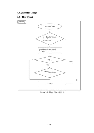
4.3.2 Algorithms
Step 1. 𝑛 ← 𝑙𝑒𝑛𝑔𝑡ℎ of List 𝐴, 𝑟 ← √ 𝑛 ,𝑠 = 0 .
Step 2. Divide the list 𝐴 in 𝑟 part and every part have 𝑟 item in that list.
Step 3. 𝑓𝑜𝑟(𝑝 = 1 𝑡𝑜 𝑟, 𝑝 + +) Part of list 𝐴 individual sort, with the Merge sort or
other Algorithms.
𝑚𝑒𝑟𝑔𝑒(𝑝𝑎𝑟𝑡. 𝑝)
Step 4. The first item will compare with the first item of seconds part.
𝑓𝑜𝑟(𝑝 = 1 𝑡𝑜 𝑟, 𝑝 + +){
𝑓𝑜𝑟(𝑖 = 1 𝑡𝑜 𝑟, 𝑖 + +){
𝑖𝑓(𝑝𝑎𝑟𝑡. (𝑝)[𝑖] ≤ 𝑝𝑎𝑟𝑡. (𝑝 + 1)[𝑠]){
𝑠 + +
}𝑒𝑙𝑠𝑒{
𝐴 ← 𝑝𝑎𝑟𝑡. (𝑖)[1]
𝐵 ← 𝑝𝑎𝑟𝑡. (𝑖 + 1)[𝑠]
𝑝𝑎𝑟𝑡. (𝑖 + 1)[𝑠] ← 𝐴
𝑝𝑎𝑟𝑡. (𝑝)[𝑖] ← 𝐵
𝑚𝑒𝑟𝑔𝑒(𝑝𝑎𝑟𝑡. (𝑖 + 1))
}
}
𝑠 = 0
}
Step 5. Return A
4.4 Complexity Analysis
The complexity of a sorting algorithm measures the running time as a
function of the number of n items to be sorted, each sorting algorithm S will be
made up of the following operations, where A1, A2...An contain the items to be
sorted and B is an auxiliary location.
Comparison which test whether Ai < Ai or test whether Ai < B.
Interchange which switch the contents of Ai and Aj or Ai and B.
Assignment which set B = Ai and then set Aj = B or Aj = Ai.
Generally the complexity function measures only the number of comparison,
since the number of other operations is at most a constant factor of the number of
other operations is at most a constant factor of the number of comparison,
Suppose space is fixed for one algorithm then only run time will be considered
for obtaining the complexity of algorithm. [27, 17]
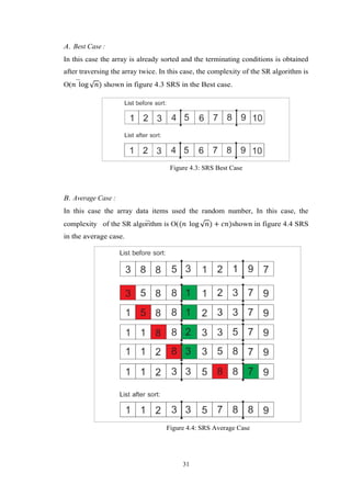
Complexity analysis of the proposed SR Sorting Algorithm for best case and
worstcase is discussed here with the help of examples.](https://image.slidesharecdn.com/srs-170016511-190723185008/85/Square-Root-Sorting-Algorithm-41-320.jpg)
![35
CHAPTER 5
Results and Discussion
5.1 Introduction
After development and implementation of SR Algorithm, We have decided to
compare this algorithm with one of the best existed algorithm that is currently
using for sorting. For this purpose we have chosen the Merge Sort algorithm
because this algorithm is one of the most powerful algorithms in terms of time
complexity, furthermore, Merge Sort can be used in an internal and external
memory.
5.2 Compare SR Sorting Algorithm with other Sorting Algorithm
(Merge Sort)
Which sorting algorithm is the fastest? This question doesn’t have an easy or
unambiguous answer, however. The speed of sorting can depend quite heavily on
the environments where the sorting is done, the type of items that are sorted and
the distribution of these items.
For example, sorting a database which is so big that can-not fit into memory all
at once is quite different from sorting an array of 100 integers, not only will the
implementation of the algorithm be quite different, naturally, but it may even be
that the same algorithm which is fast in one case is slow in the other. Also sorting
an array may be different from sorting a linked list, for example. [9]
In order to better understand the advantages and disadvantages of an algorithm,
there is a need for time that the algorithm should be adapted in different criteria’s
so that the results obtained can be examined in order to understand the
advantages and dis- advantages of the algorithm. When we discuss the complexity
of the SR algorithm, we have achieved the results after it was implemented in
Java programming language which indicates that the algorithm performs a
comparative and substitute comparison with previous algorithms. This al- growth
can still be called a technique that replaces any sorting algorithm that exists up to
now or in the future in order to reduce the time complexity of the algorithm and
when we compare merge sort with this algorithm, the results obtained from 100 to
102400 data items are presented in the following way figure 5.1, figure 5.2 and
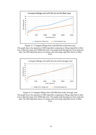
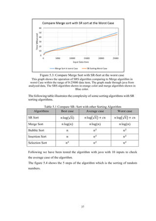
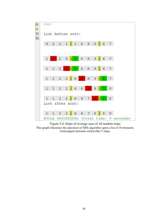
figure 5.3 compare merge sort with SRS algorithm:](https://image.slidesharecdn.com/srs-170016511-190723185008/85/Square-Root-Sorting-Algorithm-46-320.jpg)
![40
References
[1] A.A.Puntambekar. (2007). Advance Data Structures.
[2] A.A.Puntambekar. (2009). Data Structures And Algorithms.
[3] Abdel-hafeez, S. and Gordon-Ross, A. (2014). A Comparison-Free Sorting Algorithm. IEEE Journals.
[4] www.techopedia.com. (2019). Algorithm. [online] Available at:
https://www.techopedia.com/definition/3739/algorithm. [Accessed 1 Oct. 2018].
[5] www.medium.com. (2018). Algorithm Time Complexity and Big O Notation. [online] Available at:
http://https:/ /medium.com/StueyGK/algorithm-time-complexity-and-big-o-notation-51502e612b4d
[Accessed 15 Oct. 2018].
[6] www.tutorialspoint.com. (2018). Analysis of Algorithms.. [online] Available at:
https://www.tutorialspoint.com/design_and_analysis_ of_algorithms/analysis_of_algorithms.htm [Accessed 8
Oct. 2018].
[7] N. Baitipuli, V. (2009). Introduction to Data Structures Using C.
[8] www.studytonight.com. (2018). Bubble Sort Algorithm. [online] Available at:
https://www.studytonight.com/data-structures/bubble- sort [Accessed 9 Nov. 2018].
[9] www.warp.povusers.org. (2018). Comparison of several sorting algorithms. [online] Available at:
http://warp.povusers.org/SortComparison [Accessed 13 Nov. 2018].
[10] Computer Science : An Overview. (2011). PediaPress GmbH, Boppstrasse 64 , Mainz, Germany: PediaPress.
[11] Joshi (2010). Data Structures and Algorithms Using C. Tata McGraw-Hill Education.
[12] Joshi (2011). DATA STRUCTURES THROUGH C++. Tata McGraw-Hill Education.
[13] Erik Azar and Mario Eguiluz Alebicto (2016). Swift Data Structure and Algorithms. Paket.
[14] Robert Slade (2006). The Information Security Dictionary. Elsevie.
[15] www.hackerearth.com. (2018). Insertion Sort Algorithm. [online] Available at:
https://www.hackerearth.com/practice/algorithms/sorting/insertion-sort/tutorial/ [Accessed 9 Nov. 2018].
[16] Johnsonbaugh (2007). Discrete Mathematics, 6/E. India: Pearson Education.
[17] Seymour Lipschutz (2011). Data Structures with C. Data Mcgraw Hill Education Private Lmited.
[18] Dheeraj Mehrotra and Yogita Mehrotra (2008). S.Chand’s Rapid Revision in ISC Computer Science for Class
12. S. Chand Publishing.
[19] Arjun Sawhney, Rayner Vaz, Viraj Shah and Rugved Deolekar (2017). Big-O Analysis of Algorithms. IEEE
Journals.
[20] Sartaj Sahni (2005). Data Structures, Algorithms, and Applications in C++. Silicon Press.
[21] Saleh Abdel-Hafeez and Ann Gordon-Ross (2017). An Efcient O(N) Comparison-Free Sorting
Algorithm. IEEE Journals.
[22] www.codingeek.com. (2019). SHELL SORT ALGORITHM- EXPLANATION, IMPLEMENTATION AND
COM- PLEXIT. [online] Available at: https://www.codingeek.com/algorithms/shell-sort-algorithm-
explanation-implementation-and-complexity/ [Accessed 14 Nov. 2018].
[23] Edwin D. Reilly (2004). Concise Encyclopedia of Computer Science. John Wiley & Sons.
[24] www.lcm.csa.iisc.ernet.i. (2018). Sorting Methods. [online] Available at:
http://lcm.csa.iisc.ernet.in/dsa/node193.html [Accessed 19 Nov. 2018].
[25] Thomas H.. Cormen, Thomas H Cormen, Charles E Leiserson, Ronald L Rivest and Clifford Stein
(2009). Introduction To Algorithms. MIT Press.
[26] Saleh Abdel-Hafeez and Ann Gordon-Ross (2014). A Comparison sorting Algirthm. IEEE Journals.
[27] Saleh Abdel-Hafeez and Ann Gordon-Ross (2017). An Efcient O(N) Comparison-Free Sorting
Algorithm. IEEE Journals.](https://image.slidesharecdn.com/srs-170016511-190723185008/85/Square-Root-Sorting-Algorithm-51-320.jpg)
![41
[28] Gianni Franceschini and Viliam Geffert (2003). An In-Place Sorting with O(nlogn) Comparisons and O(n)
Moves.IEEE Journals.
[29] Wang Xiang (2011). Analysis of the Time Complexity of Quick Sort Algorithm. IEEE Journals.
[30] Rayner Vaz, Viraj Shah, Arjun Sawhney and Rugved Deolekar (2017). Automated Big-O Analysis of
Algorithms. IEEE Journals.
[31] S.-S.Chen, C.-H.Yang and S.-J.Chen (2000). Bubble-sort approach to channel routing. IEE Journals.
[32] Indradeep Hayaran and Pritee Khanna (2016). Couple Sort. PDGC Journals.
[33] Liu Shenghui, Ma Junfeng and CheNan (2013). Internal Sorting Algorithm for Large-scale Data Based on
GPU -assisted. IEEE Journals.
[34] Hoda Osama, Yasser Omar and Amr Badr (2016). Mapping Sorting Algorithm. IEEE Journals.
[35] Vignesh R, and Tribikram Pradhan (2016). Merge Sort Enhanced In Place Sorting Algorithm. ICACCCT.
[36] Sultan Ullah, Muhammad A. Khan and Mudasser A. Khan, H. Akbar, and Syed S. Hassan (2015). Optimized
Selection Sort Algorithm for Two Dimensional Array. IEEE journal.
[37] Neetu Faujdar and Shipra Saraswat (2017). The Detailed Experimental Analysis of Bucket Sort. IEEE
journal.
[38] Taras Dyvak (2008). The Rapid Algorithm of the Files Comparison with the Hash Functions Usage. TCSET.
[39] V.P.Kulalvaimozhi, M.Muthulakshmi, R.Mariselvi, G.Santhana Devi, C.Rajalakshmi and C.Durai (2015).
PERFORMANCE ANALYSIS OF SORTING ALGORITHM. IJCSMC Journal.
[40] www.quora.com. (2018). What is complexity of algorithm. [online] Available at:
https://www.quora.com/What- is- complexity- of-algorithm [Accessed 2 Nov. 2018].
[41] Mark Allen Weiss (2007). Data Structures and Algorithm Analysis in Java. Pearson/Addison-Wesle.
[42] www.scanftree.com. (2019). Operations on data structures. [online] Available at:
http://scanftree.com/Data_Structure [Accessed 5 Jun. 2019].](https://image.slidesharecdn.com/srs-170016511-190723185008/85/Square-Root-Sorting-Algorithm-52-320.jpg)
![42
Appendix A: Source Code
package rootsort;
import java.util.Arrays;
import java.util.Random;
/**
*
@author Mir Omranudin Abhar
*/
public class RootSort {
public static final String RED = "u001B[41m";
public static final String BLACK = "u001B[47m";
public static final String BGREEN = "u001B[42m";
static int com = 0;
static int swapp = 0;
public static void main(String[] args) {
// TODO code application logic here
// list of item
// int array[] = {
//// 1, 2, 3, 4, 5, 6, 7, 8, 9, 10
// 10,9,8,7,6,5,4,3,2,1
// };
////
int size = 10;
int array[] = new int[size];
RootSort obj = new RootSort();
// base,worst, average
obj.setArray(array, size, "average");
// Getting the size of list and getting the Sqaure root
int i = array.length;
int item = (int) Math.ceil(Math.sqrt(i));
int part = (int) Math.ceil((i / item)) + 1;
// Create the object of class for accessing the method of the class
// Show the list before sorted.
System.out.print("nList before sort: ");
obj.printList(array, item);
// This method used for sorting every part of list
obj.sortAllRow(array, part, item);
// This method used for comparing.
obj.compaireTwoPart(array, part, item);
// This loop used for showing the sorted list.
System.out.print("nList after sort: ");
obj.printList(array, item);
// System.out.println("Total Comparing : " + com);
// System.out.println("Total Swapping : " + swapp);](https://image.slidesharecdn.com/srs-170016511-190723185008/85/Square-Root-Sorting-Algorithm-53-320.jpg)
![43
}
// This methtod used for comparing.
public void compaireTwoPart(int array2D[], int part, int item) {
int max = 0, min = 0, vc = 0, vr = 0, i = 1, last = 0;
for (int row = 0; row < array2D.length; row += item) {
last = row;
for (int col = row; col < ((col >= array2D.length) ? array2D.length - 1 : row + item); col++) {
for (int rowV = row + item; rowV < array2D.length; rowV += item) {
for (int colV = rowV; colV < ((colV >= array2D.length) ? array2D.length - 1 :
rowV + item); colV++) {
vc = colV;
vr = colV;
com++;
if (array2D[col] > array2D[colV]) {
swapp++;
for (int rowVJ = row + item + item; rowVJ < array2D.length; rowVJ += item) {
for (int colVJ = rowVJ; colVJ < ((colVJ >= array2D.length) ?
array2D.length - 1 : rowVJ + item); colVJ++) {
com++;
if (array2D[vc] > array2D[colVJ]) {
vc = colVJ;
vr = colVJ;
}
break;
}
}
max = array2D[col];
min = array2D[vc];
i++;
int ll = 1;
System.out.println("");
System.out.println("");
for (int j = 0; j < array2D.length; j++) {
if (j == item * i) {
i++;
}
if (j == col) {
System.out.print(RED + " " + array2D[j] + " " + BLACK);
} else if (j == vc) {
System.out.print(BGREEN + " " + array2D[j] + " " + BLACK);
} else {
System.out.print(" " + array2D[j] + " ");
}
if (ll * item == j + 1) {
System.out.print("u001B[43m" + "|" + BLACK);](https://image.slidesharecdn.com/srs-170016511-190723185008/85/Square-Root-Sorting-Algorithm-54-320.jpg)
![44
ll++;
}
}
array2D[vc] = max;
array2D[col] = min;
Arrays.sort(array2D, vr, ((vr + item > array2D.length) ? array2D.length : vr +
item));
break;
} else {
break;
}
}
}
}
}
}
public void printList(int array[], int item) {
int i = 1;
System.out.println("n");
for (int j = 0; j < array.length; j++) {
if (j == item * i) {
i++;
System.out.print("u001B[43m" + "|" + BLACK);
}
System.out.print(BLACK + " " + array[j] + " ");
}
System.out.println("");
}
// This method used for sorting every part of list
public void sortAllRow(int array2D[], int part, int item) {
int i = 1;
int cc = 0;
for (int row = 0; row <= part; row++) {
if (item * i >= array2D.length) {
if ((item * i) - item < array2D.length) {
cc = array2D.length;
} else {
break;
}
} else {
cc = item * i;
}
Arrays.sort(array2D, item * row, (cc));
i++;
}](https://image.slidesharecdn.com/srs-170016511-190723185008/85/Square-Root-Sorting-Algorithm-55-320.jpg)
![45
}
// This method used for sorting every part of list
public void setArray(int array[], int size, String Case) {
Random rand = new Random();
if (Case.equals("best")) {
// Base Case
for (int set = 0; set < size; set++) {
array[set] = set;
}
} else if (Case.equals("worst")) {
// Worst Case
for (int set = 0; set < size; set++) {
array[set] = size - set;
}
} else {
// Random Case
for (int set = size - 1; set >= 0; set--) {
array[set] = rand.nextInt(10);
}
}
}
}](https://image.slidesharecdn.com/srs-170016511-190723185008/85/Square-Root-Sorting-Algorithm-56-320.jpg)