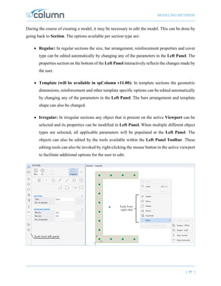
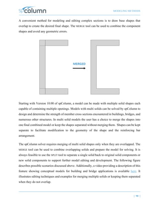
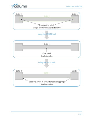
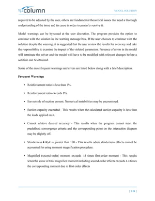
The document is a user manual for the Spcolumn software, designed for the structural analysis and design of reinforced concrete sections under axial and flexural loads, supporting various codes. It details program features, including capabilities for handling different geometries, importing/exporting materials, and analysis methods with a focus on slenderness effects. The software is applicable for diverse engineering structures like columns, shear walls, and bridge piers, and emphasizes user responsibility for the integrity of the modeling and data input.


![INTRODUCTION
| 10 |
1.4. Terms & Conventions
The following terms are used throughout this manual. A brief explanation is given to help
familiarize you with them.
Windows refers to the Microsoft Windows environment as listed in System
Requirements.
[ ] indicates metric equivalent
Click on means to position the cursor on top of a designated item or
location and press and release the left-mouse button (unless
instructed to use the right-mouse button).
Double-click on means to position the cursor on top of a designated item or
location and press and release the left-mouse button twice in quick
succession.
To help you locate and interpret information easily, the spColumn manual adheres to the following
text format.
Italic indicates a glossary item, or emphasizes a given word or phrase.
Bold indicates the name of a menu or a menu item command such as
File or Save.
Mono-space indicates something you should enter with the keyboard. For
example “c:*.txt”.
KEY + KEY indicates a key combination. The plus sign indicates that you
should press and hold the first key while pressing the second key,
then release both keys. For example, “ALT + F” indicates that you
should press the “ALT” key and hold it while you press the “F”
key. then release both keys.
SMALL CAPS Indicates the name of an object such as a dialog box or a dialog
box component. For example, the OPEN dialog box or the CANCEL
or MODIFY buttons.](https://image.slidesharecdn.com/spcolumn-manual-240518140157-ee4e4ec0/85/spColumn-Manual-design-column-by-spcolumn-software-pdf-10-320.jpg)
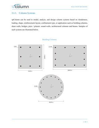

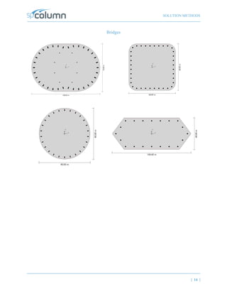
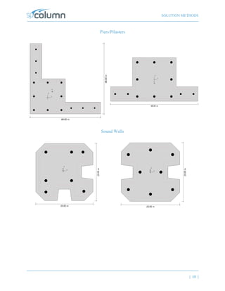
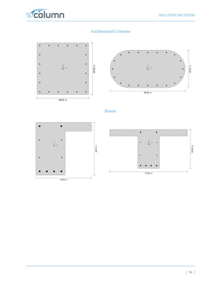
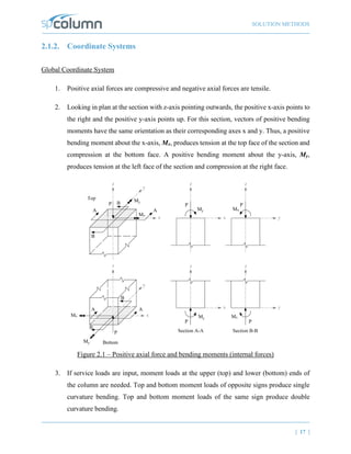


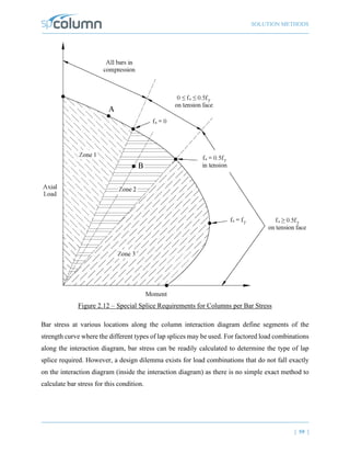
![SOLUTION METHODS
| 21 |
Output Phase
The program does not perform any geometric checks during output phase. However, any warning
pertaining to model adequacy, stability, or exceedance of limits is reported.
2.2.3. Definitions and Assumptions
1. The analysis of the reinforced concrete section performed by spColumn conforms to the
provisions of the Strength Design Method1
and Unified Design Provisions2
and is based
on the following assumptions.
a) All conditions of strength satisfy the applicable conditions of equilibrium and strain
compatibility3
b) Strain in the concrete and in the reinforcement is directly proportional to the distance
from the neutral axis4
. In other words, plane sections normal to the axis of bending
are assumed to remain plane after bending.
c) The maximum usable (ultimate) strain at the extreme concrete compression fiber is
assumed equal to 0.003 for ACI codes5
and 0.0035 for CSA codes6
unless otherwise
specified by the user.
1
For CSA A23.3-19 (Ref. [18]) CSA A23.3-14 (Ref. [16]) CSA A23.3-04 (Ref. [8]) and CSA A23.3-94 (Ref.[9])
2
For ACI 318-19 (Ref. [1]), ACI 318-14 (Ref. [2]), ACI 318-11 (Ref. [3]), ACI 318-08 (Ref. [4]), ACI 318-05 (Ref.
[5]) and ACI 318-02 (Ref. [6]); also see notes on ACI 318-08, 8.1.2 in Ref. [11] and notes on ACI 318-11, 8.1.2 in
Ref. [15]
3
ACI 318-19, 4.5.1, 22.2.1.1, 13.2.6.4; ACI 318-14, 4.5.1, 22.2.1.1, 13.2.6.2; ACI 318-11, 10.2.1; ACI 318-08,
10.2.1; ACI 318-05, 10.2.1; ACI 318-02, 10.2.1; CSA A23.3-19, 10.1.1; CSA A23.3-14, 10.1.1; CSA A23.3-04,
10.1.1; CSAA23.3-94, 10.1.1
4
ACI 318-19, 22.1.2, 22.2.1.2; ACI 318-14, 22.1.2, 22.2.1.2; ACI 318-11, 10.2.2; ACI 318-08, 10.2.2; ACI 318-05,
10.2.2; ACI 318-02, 10.2.2; CSAA23.3-19, 10.1.2; CSAA23.3-14, 10.1.2; CSAA23.3-04, 10.1.2; CSAA23.3-94,
10.1.2
5
ACI 318-19, 22.2.2.1; ACI 318-14, 22.2.2.1; ACI 318-11, 10.2.3; ACI 318-08, 10.2.3; ACI 318-05, 10.2.3; ACI
318-02, 10.2.3
6
CSAA23.3-19, 10.1.3; CSAA23.3-14, 10.1.3; CSAA23.3-04, 10.1.3; CSAA23.3-94, 10.1.3](https://image.slidesharecdn.com/spcolumn-manual-240518140157-ee4e4ec0/85/spColumn-Manual-design-column-by-spcolumn-software-pdf-21-320.jpg)
![SOLUTION METHODS
| 22 |
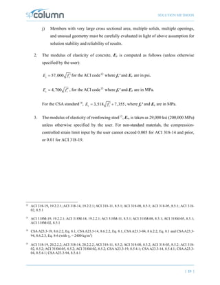
d) A uniform rectangular concrete stress block is used. For ACI code7
, the maximum
uniform concrete compressive stress, fc, is 0.85 fc' by default and the block depth is
β1c, where c is the distance from the extreme compression fiber to the neutral axis
and β1 is described in item 4 below. For CSA8
, fc is taken as:
( )
0.85 0.0015 0.68
c c c c
f f f f
′ ′ ′
=
− ≥ , where fc' is in MPa
Both fc and β1 can be modified by the user.
e) Concrete displaced by the reinforcement in compression is deducted from the
compression block9
f) For the reinforcing steel, the elastic-plastic stress-strain distribution is used10
. Stress
in the reinforcing steel below the yield strength, fy, is directly proportional to the
strain. For strains greater than that corresponding to the yield strength, the
reinforcement stress remains constant and equal to fy. Reinforcing steel yield
strength must be with in customary ranges.
g) Tensile strength of concrete in axial and flexural calculations is neglected11
.
h) Reinforcement bars are located within section outline.
i) Irregular sections must be composed of a closed polygon without any intersecting
sides.
7
ACI 318-19, 22.2.2.3; ACI 318-14, 22.2.2.3; ACI 318-11, 10.2.6; ACI 318-08, 10.2.6, 10.2.7; ACI 318-05, 10.2.6,
10.2.7; ACI 318-02, 10.2.6, 10.2.6
8
CSAA23.3-19, 10.1.1; CSAA23.3-14, 10.1.1; CSAA23.3-04, 10.1.1; CSAA23.3-94, 10.1.1
9
For consistency with Eq. 22.4.2.4 in ACI codes (Refs. [1], [2]) and for consistency with Eq. 10-1 and 10-2 in ACI
codes (Refs. [3], [4], [5], [6]) and with Eq. 10-10 in CSA codes (Refs. [8], [9])
10
ACI 318-19, 20.2.2.1; ACI 318-14, 20.2.2.1; ACI 318-11, 10.2.4; ACI 318-08, 10.2.4; ACI 318-05, 10.2.4; ACI
318-02, 10.2.4; CSA A23.3-19, 8.5.3.2; CSA A23.3-14, 8.5.3.2; CSA A23.3-04, 8.5.3.2; CSA A23.3-94, 8.5.3.2
11
ACI 318-19, 22.2.2.2; ACI 318-14, 22.2.2.2; ACI 318-11, 10.2.5; ACI 318-08, 10.2.5; ACI 318-05, 10.2.5; ACI
318-02, 10.2.5; CSAA23.3-19, 10.1.5; CSAA23.3-14, 10.1.5; CSAA23.3-04, 10.1.5; CSA A23.3-94, 10.1.5](https://image.slidesharecdn.com/spcolumn-manual-240518140157-ee4e4ec0/85/spColumn-Manual-design-column-by-spcolumn-software-pdf-22-320.jpg)
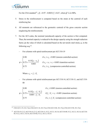


![SOLUTION METHODS
| 39 |
2. The program starts the design by trying the smallest section (minimum dimensions) and
the least amount of reinforcing bars. The program verifies that the ratio of provided
reinforcement is always within the specified minimum and maximum ratios.
Furthermore, unless otherwise specified by the user29
, the bar spacing is always kept
greater than or equal to the larger of 1.5 times the bar diameter or 1.5 in. [40 mm] for
ACI30
and 1.4 times the bar diameter or 1.2 in [30 mm] for CSA31
.
3. A section fails the design if, for any load point the capacity ratio exceeds 1.0 (unless
otherwise specified in the Design Criteria dialog box).
4. Once a section passes the design, its capacity is computed and the calculations explained
in the procedure for section investigation are performed.
5. For members with large cross-sectional area spColumn sometimes warns the user with the
following message “Cannot achieve desired accuracy”. This results when the program
cannot meet the predefined convergence criteria and the corresponding point on the
interaction diagram may be slightly off. The convergence criteria is more stringent than
required in engineering practice, however, the shape of the interaction diagram should be
verified to be relatively smooth and free of unexpected discontinuity.
29
The user may select spacing greater than the default value to take into account tolerances for reinforcement
placement (see ACI 117-06, Ref [7]) and other project specific considerations.
30
ACI 318-19, 25.2.3; ACI 318-14, 25.2.3; ACI 318-11, 7.6.3; ACI 318-08, 7.6.3; ACI 318-05, 7.6.3; ACI 318-02,
7.6.3
31
CSAA23.3-19, Annex A, 6.6.5.2; CSAA23.3-14, Annex A, 6.6.5.2; CSAA23.3-04, Annex A, 6.6.5.2; CSAA23.3-
94, Annex A, A12.5.2](https://image.slidesharecdn.com/spcolumn-manual-240518140157-ee4e4ec0/85/spColumn-Manual-design-column-by-spcolumn-software-pdf-39-320.jpg)
![SOLUTION METHODS
| 40 |
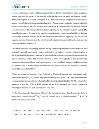
2.3.3. Moment Magnification at Ends of Compression Member
This procedure accounts for moment magnification due to second-order effects at ends of columns
in sway frames32
.
1. If properties of framing members are input, spColumn computes the effective length
factor, ks, for sway condition using the following equation33
:
( )
2
/
1 tan 0
36 6
s A B A B
s s
k
k k
π ψ ψ ψ ψ
π π
+
− − =
where ψ is the ratio of ∑(EI/ℓc) of columns to ∑(EI/ℓ) of beams in a plane at one end of
the column, ψA and ψB are the values of ψ at the upper end and the lower end of the
column. For a hinged end, ψ is very large. This happens in the case where ∑(EI/ℓ) of
beams is very small (or zero) relative to the ∑(EI/ℓc) of columns at that end. In this case,
the program outputs 999.9 for the value of ψ. The moment of inertia used in computing ψ
is the gross moment of inertia multiplied by the cracked section coefficients34
(specified
in the Slenderness Factors dialog box).
2. For the ACI code35
, slenderness effects will be considered if / 22.0
u
k l r
× ≥ . For the
CSA standards, all sway columns are designed for slenderness effects.
32
ACI 318-19, 6.6.4.6.1; ACI 318-14, 6.6.4.6.1; ACI 318-11, 10.10.7; ACI 318-08, 10.10.7; ACI 318-05, 10.13; ACI
318-02, 10.13; CSAA23.3-19, 10.16; CSAA23.3-14, 10.16; CSAA23.3-04, 10.16; CSA A23.3-94, 10.16
33
Exact formula derived in Ref. [14] pp. 851 for Jackson and Moreland alignment chart
34
ACI 318-19, 6.6.3.1.1, 6.6.4.2, 6.7.1.3, 6.8.1.4; ACI 318-14, 6.6.3.1.1, 6.6.4.2, 6.7.1.3, 6.8.1.4; ACI 318-11,
10.10.4.1; ACI 318-08, 10.10.4.1; ACI 318-05, 10.11.1, 10.13.1; ACI 318-02, 10.11.1, 10.13.1; CSA A23.3-14,
10.14.1.2, 10.16.1; CSAA23.3-19, 10.14.1.2, 10.16.1; CSA A23.3-04, 10.14.1.2, 10.16.1; CSAA23.3-94, 10.14.1,
10.16.1
35
ACI 318-19, 6.2.5; ACI 318-14, 6.2.5; ACI 318-11, 10.10.1; ACI 318-08, 10.10.1; ACI 318-05, 10.13.2; ACI 318-
02, 10.13.2](https://image.slidesharecdn.com/spcolumn-manual-240518140157-ee4e4ec0/85/spColumn-Manual-design-column-by-spcolumn-software-pdf-40-320.jpg)

![SOLUTION METHODS
| 42 |
6. Flexural stiffness EI is calculated as39
:
0.2
1
c g s se
ds
E I E I
EI
β
+
=
+
where Ec is the modulus of elasticity of concrete, Es is the modulus elasticity of steel, Ig is
the gross moment of inertia of the concrete section, Ise is the moment of inertia of
reinforcement. Assuming that shear due to lateral loads is not sustained in most frames40
,
the βds is taken as zero (with the exception of strength and stability of the structure as a
whole under factored gravity loads described in Step 11).
7. The critical buckling load, Pc, is computed as41
.
( )
2
2
c
u
EI
P
k l
π
=
×
39
ACI 318-19, 6.6.4.4.4, Eq. 6.6.4.4.4b; ACI 318-14, 6.6.4.4.4, Eq. 6.6.4.4.4b; ACI 318-11, 10.10.6 Eq. 10-14; ACI
318-08, 10.10.6 Eq. 10-14; ACI 318-05, 10.12.3 Eq. 10-11; ACI 318-02, 10.12.3. Eq. 10-10; CSA A23.3-14/19,
10.16.3.2, 10.15.3 Eq. 10-19; CSA A23.3-04, 10.16.3.2, 10.15.3 Eq. 10-18; CSA A23.3-94, 10.16.3.2, 10.15.3.1
Eq. 10-18
40
ACI 318-19, R6.6.4.6.2(b); ACI 318-14, R6.6.4.6.2(b); ACI 318-11, R10.10.7.4; ACI 318-08, R10.10.7.4;ACI 318-
05, R10.13.4.1, R10.13.4.3; ACI 318-02, R10.13.4.1, R10.13.4.3; Ref. [10] pp 586 (first paragraph from the
bottom)
41
ACI 318-19, 6.6.4.4.2, Eq. 6.6.4.4.2; ACI 318-14, 6.6.4.4.2, Eq. 6.6.4.4.2; ACI 318-11, 10.10.6 Eq. 10-13; ACI
318-08, 10.10.6 Eq. 10-13; ACI 318-05, 10.12.3 Eq. 10-10; ACI 318-02, 10.12.3 Eq. 10-10; CSA A23.3-19,
10.16.3.2, 10.15.3.1 Eq. 10-18; CSAA23.3-14, 10.16.3.2, 10.15.3.1 Eq. 10-18; CSA A23.3-04, 10.16.3.2, 10.15.3.1
Eq. 10-17; CSAA23.3-94, 10.16.3.2, 10.15.3 Eq. 10-17](https://image.slidesharecdn.com/spcolumn-manual-240518140157-ee4e4ec0/85/spColumn-Manual-design-column-by-spcolumn-software-pdf-42-320.jpg)


![SOLUTION METHODS
| 45 |
2.3.4. Moment Magnification along Length of Compression Member
This procedure accounts for moment magnification due to second-order effect along the length of
compression members that are part of either nonsway47
or sway frames48
. In nonsway frames,
moment magnification along length is neglected by the program if the condition in Step 3 is
satisfied.
In sway frames designed per ACI 318-02/05 and CSA A23.3-94/04/14/19, the magnification along
the length is neglected if49
:
35
u
u
c g
l
r P
f A
≤
′
By rearranging and introducing, ( )
/
u c g
k P f A
′ ′
= this condition can be succinctly expressed as
/ 35
u
k l r
′× ≤ . For columns designed per ACI 318-19, ACI 318-14, ACI 318-11, and ACI 318-08
codes, moment magnification along length is to be considered for all slender compression
members, i.e. columns in either nonsway or sway frames regardless of the /
u
k l r
′× ratio. Since
various published examples of columns designed per ACI 318-19, ACI 318-14, ACI 318-11, and
ACI 318-08 do not combine moment magnification at ends and along length of columns in sway
frames50
, spColumn optionally allows not considering moment magnification along the length of
acolumn in a sway frame based on engineering judgment of the user.
47
ACI 318-19, 6.6.4.4.2, 6.6.4.5.1, 6.6.4.5.2; ACI 318-14, 6.6.4.4.2, 6.6.4.5.1, 6.6.4.5.2; ACI 318-11, 10.10.6; ACI
318-08, 10.10.6; ACI 318-05, 10.12; ACI 318-02, 10.12; CSAA23.3-19, 10.15; CSA A23.3-14, 10.15; CSAA23.3-
04, 10.15; CSAA23.3-94, 10.15
48
ACI 318-19, 6.6.1.1; ACI 318-14, 6.6.1.1; ACI 318-11, 10.10.2.2; ACI 318-08, 10.10.2.2; ACI 318-05, 10.13.5;
ACI 318-02, 10.13.5; CSA A23.3-19, 10.16.4; CSA A23.3-14, 10.16.4; CSA A23.3-04, 10.16.4; CSA A23.3-94,
10.16.4
49
ACI 318-05, Eq. 10-19; ACI 318-02, Eq. 10-19; CSAA23.3-04, Eq. 10-26; CSAA23.3-04, Eq. 10-25; CSAA23.3-
94, Eq. 10-25
50
See Example 11.2 in Ref. [11], Example 12.4 in Ref. [13], and Example 12.3 in Ref. [12]](https://image.slidesharecdn.com/spcolumn-manual-240518140157-ee4e4ec0/85/spColumn-Manual-design-column-by-spcolumn-software-pdf-45-320.jpg)
![SOLUTION METHODS
| 46 |
When moment magnification along the length of a compression member is considered, the
following procedure is followed:
1. The effective length factor, k, is either entered by the user or calculated by the program.
The value of k must be between 0.5 and 1.0 for moment magnification along length and
the recommended51
value is 1.0. Smaller values can be used if justified by analysis. If
properties of framing members are input, spColumn computes the effective length factor,
k, for nonsway condition from the following equation52
:
( )
2
2
/ 2
1 tan 1
4 2 tan / / 2
A B A B k
k k k k
ψ ψ ψ ψ
π π π
π π
+
+ − + =
Where ψ is the ratio of ∑(EI/ℓc) of columns to ∑(EI/ℓ) of beams in a plane at one end of
the column, ψA and ψB are the values of ψ at the upper end and the lower end of the
column, respectively. Moments of inertia used in computing ψ factors are gross moments
of inertia multiplied by the cracked section coefficients53
(specified in the Slenderness
Factors dialog box).
2. Moments at column ends, M1 and M2, are calculated, where M1 is the moment with the
smaller absolute value and M2 is the moment with the larger absolute value. For columns
in nonsway frames, the end moments will be equal to the factored applied first order
moment. For columns in sway frames, the end moments will be the moments M1 and M2
calculated in the procedure for moment magnification at ends of compression member.
51
ACI 318-19, 6.6.4.4.3, R6.6.4.4.3; ACI 318-14, 6.6.4.4.3, R6.6.4.4.3; ACI 318-11, 10.10.6.3, R10.10.6.3; ACI 318-
08, 10.10.6.3, R10.10.6.3; ACI 318-05, 10.12.1; ACI 318-02, 10.12.1; CSA A23.3- 19, 10.15.1; CSA A23.3-14,
10.15.1; CSAA23.3-04, 10.15.1; CSAA23.3-94, 10.15.1
52
Exact formula derived in Ref. [14] pp. 848 for Jackson and Moreland alignment chart.
53
ACI 318-19, 6.6.3.1.1, 6.6.4.2, 6.7.1.3, 6.8.1.4; ACI 318-14, 6.6.3.1.1, 6.6.4.2, 6.7.1.3, 6.8.1.4; ACI 318-11,
10.10.4.1; ACI 318-08, 10.10.4.1; ACI 318-05, 10.11.1, 10.12.1; ACI 318-02, 10.11.1, 10.12.1; CSA A23.3-19,
10.14.1.2, CSAA23.3-14, 10.14.1.2, 10.15.1; CSAA23.3-04, 10.14.1.2, 10.15.1; CSA A23.3-94, 10.14.1, 10.15.1](https://image.slidesharecdn.com/spcolumn-manual-240518140157-ee4e4ec0/85/spColumn-Manual-design-column-by-spcolumn-software-pdf-46-320.jpg)


![SOLUTION METHODS
| 66 |
2.7. References
[1] Building Code Requirements for Structural Concrete (ACI 318-19) and Commentary (ACI
318R-19), American Concrete Institute, 2019
[2] Building Code Requirements for Structural Concrete (ACI 318-14) and Commentary (ACI
318R-14), American Concrete Institute, 2014
[3] Building Code Requirements for Structural Concrete (ACI 318-11) and Commentary (ACI
318R-11), American Concrete Institute, 2011
[4] Building Code Requirements for Structural Concrete (ACI 318-08) and Commentary (ACI
318R-08), American Concrete Institute, 2008
[5] Building Code Requirements for Structural Concrete (ACI 318-05) and Commentary (ACI
318R-05), American Concrete Institute, 2005
[6] Building Code Requirements for Structural Concrete (ACI 318-02) and Commentary (ACI
318R-02), American Concrete Institute, 2002
[7] Specification for Tolerances for Concrete and Materials and Commentary, An ACI
Standard (ACI 117-06), American Concrete Institute, 2006
[8] CSA23.3-04, Design of Concrete Structures, Canadian Standards Association, 2004
[9] CSA23.3-94, Design of Concrete Structures, Canadian Standards Association, 1994
(Reaffirmed 2000)
[10] National Building Code of Canada 2005, Volume 1, Canadian Commission on Buildings
and Fire Codes, National Research Council of Canada, 2005
[11] Notes on ACI 318-08 Building Code Requirements for Structural Concrete with Design
Applications, Edited by Mahmoud E. Kamara, Lawrence C. Novak and Basile G. Rabbat,
Portland Cement Association, 2008](https://image.slidesharecdn.com/spcolumn-manual-240518140157-ee4e4ec0/85/spColumn-Manual-design-column-by-spcolumn-software-pdf-66-320.jpg)
![SOLUTION METHODS
| 67 |
[12] Wight J.K. and MacGregor J.G., Reinforced Concrete, Mechanics and Design, Fifth
Edition, Pearson Prentice Hall, 2009
[13] Hassoun M.N. and Al-Manaseer A., Structural Concrete Theory and Design, Fourth
Edition, John Wiley & Sons, Inc., 2009
[14] Salomon C.G. and Johnson J.E., Steel Structures: Design and Behavior, 2nd Edition,
Harper & Row Publishers, 1980
[15] Notes on ACI 318-11 Building Code Requirements for Structural Concrete with Design
Applications, Edited by Mahmoud E. Kamara, and Lawrence C. Novak, Portland Cement
Association, 2013
[16] CSA23.3-14, Design of Concrete Structures, Canadian Standards Association, 2014
[17] National Building Code of Canada 2010, Volume 1, Canadian Commission on Buildings
and Fire Codes, National Research Council of Canada, 2010
[18] CSA23.3-19, Design of Concrete Structures, Canadian Standards Association, 2019](https://image.slidesharecdn.com/spcolumn-manual-240518140157-ee4e4ec0/85/spColumn-Manual-design-column-by-spcolumn-software-pdf-67-320.jpg)


![APPENDIX
| 169 |
For CSA A23.3-19 and CSA A23.3-14 codes3
:
U1 = 1.4D
U2 = 1.25D + 1.5L + 1S
U3 = 0.9D + 1.5L + 1S
U4 = 1.25D + 1.5L + 0.4W
U5 = 1.25D + 1.5L - 0.4W
U6 = 0.9D + 1.5L + 0.4W
U7 = 0.9D + 1.5L - 0.4W
U8 = 1.25D + 1L + 1.5S
U9 = 0.9D + 1L + 1.5S
U10 = 1.25D + 0.4W + 1.5S
U11 = 1.25D - 0.4W + 1.5S
U12 = 0.9D + 0.4W + 1.5S
U13 = 0.9D - 0.4W + 1.5S
U14 = 1.25D + 0.5L + 1.4W
U15 = 1.25D + 0.5L - 1.4W
U16 = 1.25D + 1.4W + 0.5S
U17 = 1.25D - 1.4W + 0.5S
U18 = 0.9D + 0.5L + 1.4W
U19 = 0.9D + 0.5L - 1.4W
U20 = 0.9D + 1.4W + 0.5S
U21 = 0.9D - 1.4W + 0.5S
U22 = 1D + 0.5L + 1E + 0.25S
U23 = 1D + 0.5L - 1E + 0.25S
3
CSA A23.3-14/19 Annex C, Table C1; NBCC 2010 [10], Table 4.1.3.2A](https://image.slidesharecdn.com/spcolumn-manual-240518140157-ee4e4ec0/85/spColumn-Manual-design-column-by-spcolumn-software-pdf-169-320.jpg)
![APPENDIX
| 170 |
For the CSA A23.3-04 code4
:
U1 = 1.4D
U2 = 1.25D + 1.5L + 0.5S
U3 = 0.9D + 1.5L + 0.5S
U4 = 1.25D + 1.5L + 0.4W
U5 = 1.25D + 1.5L - 0.4W
U6 = 0.9D + 1.5L + 0.4W
U7 = 0.9D + 1.5L - 0.4W
U8 = 1.25D + 0.5L + 1.5S
U9 = 0.9D + 0.5L + 1.5S
U10 = 1.25D + 0.4W + 1.5S
U11 = 1.25D - 0.4W + 1.5S
U12 = 0.9D + 0.4W + 1.5S
U13 = 0.9D - 0.4W + 1.5S
U14 = 1.25D + 0.5L + 1.4W
U15 = 1.25D + 0.5L - 1.4W
U16 = 1.25D + 1.4W + 0.5S
U17 = 1.25D - 1.4W + 0.5S
U18 = 0.9D + 0.5L + 1.4W
U19 = 0.9D + 0.5L - 1.4W
U20 = 0.9D + 1.4W + 0.5S
U21 = 0.9D - 1.4W + 0.5S
U22 = 1D + 0.5L + 1E + 0.25S
U23 = 1D + 0.5L - 1E + 0.25S
4
CSA A23.3-04, 8.3.2; CSAA23.3-04, Annex C, Table C1; NBCC 2005 [10], Table 4.1.3.2](https://image.slidesharecdn.com/spcolumn-manual-240518140157-ee4e4ec0/85/spColumn-Manual-design-column-by-spcolumn-software-pdf-170-320.jpg)


![APPENDIX
| 178 |
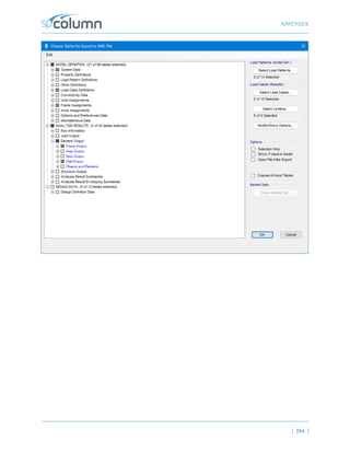
A.3. spColumn Text Input (CTI) file format
spColumn is able to read three file formats, COL, COLX and CTI and save its input data into two
file formats, COLX file or CTI file. CTI files are plain text files that can be edited by any text
editing software.
Caution must be used when editing a CTI file because some values may be interrelated. If one of
these values is changed, then other interrelated values should be changed accordingly. While this
is done automatically when a model is edited in the spColumn user graphic user interface (GUI),
one must update all the related values in a CTI file manually in order to obtain correct results. For
example, if units are changed from English to Metric in GUI, all the related input values are
updated automatically. If this is done by editing a CTI file, however, not only the unit flag but also
all the related input values must be updated manually.
The best way to create a CTI file is by using the spColumn GUI and selecting CTI file type in the
Save As menu command. Then, any necessary modifications to the CTI file can be applied with
any text editor. However, it is recommended that users always verify modified CTI files by loading
them in the spColumn GUI to ensure that the modifications are correct before running manually
revised CTI files in batch mode.
The CTI file is organized by sections. Each section contains a title in square brackets, followed by
values required by the section. The CTI file contains the following sections.
[spColumn Version]
[Project]
[Column ID]
[Engineer]
[Investigation Run Flag]
[Design Run Flag]
[Slenderness Flag]
[User Options]
[Irregular Options]
[Ties]
[Investigation Reinforcement]](https://image.slidesharecdn.com/spcolumn-manual-240518140157-ee4e4ec0/85/spColumn-Manual-design-column-by-spcolumn-software-pdf-178-320.jpg)
![APPENDIX
| 179 |
[Design Reinforcement]
[Investigation Section Dimensions]
[Design Section Dimensions]
[Material Properties]
[Reduction Factors]
[Design Criteria]
[External Points]
[Internal Points]
[Reinforcement Bars]
[Factored Loads]
[Slenderness: Column]
[Slenderness: Column Above And Below]
[Slenderness: Beams]
[EI]
[SldOptFact]
[Phi_Delta]
[Cracked I]
[Service Loads]
[Load Combinations]
[BarGroupType]
[User Defined Bars]
[Sustained Load Factors]
Each section of a CTI file and allowable values of each parameter are described in details below.
Corresponding GUI commands are presented in parenthesis.
#spColumn Text Input (CTI) File
The number sign, #, at the beginning of a line of text indicates that the line of text is a comment.
The # sign must be located at the beginning of a line. Comments may be added anywhere necessary
in a CTI file to make the file more readable. If a comment appears in multiple lines, each line must
be started with a # sign](https://image.slidesharecdn.com/spcolumn-manual-240518140157-ee4e4ec0/85/spColumn-Manual-design-column-by-spcolumn-software-pdf-179-320.jpg)
![APPENDIX
| 180 |
[spColumn Version]
Reserved. Do not edit.
[Project]
There is one line of text in this section.
Project name (Project left panel | Description)
[Column ID]
There is one line of text in this section.
Column ID (Project left panel | Description)
[Engineer]
There is one line of text in this section.
Engineer name (Project left panel | Description)
[Investigation Run Flag]
Reserved. Do not edit.
[Design Run Flag]
Reserved. Do not edit.
[Slenderness Flag]
Reserved. Do not edit.](https://image.slidesharecdn.com/spcolumn-manual-240518140157-ee4e4ec0/85/spColumn-Manual-design-column-by-spcolumn-software-pdf-180-320.jpg)
![APPENDIX
| 181 |
[User Options]
There are 27 values separated by commas in one line in this section. These values are described
below in the order they appear from left to right.
1. 0-Investigation Mode; 1-Design Mode; (Run Option in Project left panel | Run Options)
2. 0-English Unit; 1-Metric Units; (Unit system in Project left panel | General)
3. 0-ACI 318-02; 1- CSA A23.3-94; 2-ACI 318-05; 3-CSA A23.3-04; 4-ACI 318-08; 5-ACI
318-11; 6-ACI 318-14; 7-CSA A23.3-14; 8-ACI 318-19; 9-CSA A23.3-19 (Design Code
in Project left panel | General)
4. 0-X Axis Run; 1-Y Axis Run; 2-Biaxial Run; (Run Axis in Project left panel | Run Options)
5. Reserved. Do not edit.
6. 0-Slenderness is not considered; 1-Slenderness in considered; (Consider Slenderness in
Project left panel | Run Options)
7. 0-Design for minimum number of bars; 1-Design for minimum area of reinforcement; (Bar
selection in Definitions dialog | Properties | Design Criteria | Reinforcement Bars)
8. Reserved. Do not edit.
9. 0-Rectangular Column Section; 1-Circular Column Section; 2-Irregular Column Section;
(Section left panel)
10. 0-Rectangular reinforcing bar layout; 1-Circular reinforcing bar layout; (Layout in Section
left panel | Rect. Or Cir. | Bar Arrangement - when Type is All Sides Equal)
11. 0-Structural Column Section; 1-Architectural Column Section; 2-User Defined Column
Section; (Column Type in Definitions dialog | Properties | Design Criteria)
12. 0-Tied Confinement; 1-Spiral Confinement; 2-Other Confinement; (Confinement in
Definitions dialog | Properties | Reduction Factors | Confinement)](https://image.slidesharecdn.com/spcolumn-manual-240518140157-ee4e4ec0/85/spColumn-Manual-design-column-by-spcolumn-software-pdf-181-320.jpg)

![APPENDIX
| 183 |
26. Number of load combinations; (Load combinations in Definitions dialog | Load
Case/Combo)
27. Section capacity: 0-Moment capacity method; 1-Critical Capacity method; (Section
capacity in Project left panel | General)
[Irregular Options]
There are 13 values separated by commas in one line in this section. These values are described
below in the order they appear from left to right. (Section left panel | Irregular)
1. Reserved. Do not edit.
2. Reserved. Do not edit.
3. Reserved. Do not edit.
4. Reserved. Do not edit.
5. Area of reinforcing bar that is to be added through irregular section editor
6. Maximum X value of drawing area of irregular section editor
7. Maximum Y value of drawing area of irregular section editor
8. Minimum X value of drawing area of irregular section editor
9. Minimum Y value of drawing area of irregular section editor
10. Grid step in X of irregular section editor
11. Grid step in Y of irregular section editor
12. Grid snap step in X of irregular section editor
13. Grid snap step in Y of irregular section editor](https://image.slidesharecdn.com/spcolumn-manual-240518140157-ee4e4ec0/85/spColumn-Manual-design-column-by-spcolumn-software-pdf-183-320.jpg)
![APPENDIX
| 184 |
[Ties]
There are 3 values separated by commas in one line in this section. These values are described
below in the order they appear from left to right. (Section left panel | Rect. or Cir. | Cover Type)
1. Index (0 based) of tie bars for longitudinal bars smaller that the one specified in the 3rd
item
in this section in the drop-down list
2. Index (0 based) of tie bars for longitudinal bars bigger that the one specified in the 3rd
item
in this section in the drop-down list
3. Index (0 based) of longitudinal bar in the drop-down list
[Investigation Reinforcement]
This section applies to investigation mode only. There are 12 values separated by commas in one
line in this section. These values are described below in the order they appear from left to right.
If Side Different (Type is Sides Different in Section left panel | Rect. | Bar Arrangement) is
selected:
1. Number of top bars
2. Number of bottom bars
3. Number of left bars
4. Number of right bars
5. Index (0 based) of top bars (Top Bar Size drop-download list)
6. Index (0 based) of bottom bars (Bottom Bar Size drop-download list)
7. Index (0 based) of left bars (Left Bar Size drop-download list)
8. Index (0 based) of right bars (Right Bar Size drop-download list)](https://image.slidesharecdn.com/spcolumn-manual-240518140157-ee4e4ec0/85/spColumn-Manual-design-column-by-spcolumn-software-pdf-184-320.jpg)

![APPENDIX
| 186 |
[Design Reinforcement]
This section applies to design mode only. There are 12 values separated by commas in one line in
this section. These values are described below in the order they appear from left to right.
If Side Different (Type is Sides Different in Section left panel | Rect. | Bar Arrangement) is
selected:
1. Minimum number of top and bottom bars
2. Maximum number of top and bottom bars
3. Minimum number of left and right bars
4. Maximum number of left and right bars
5. Index (0 based) of minimum size for top and bottom bars
6. Index (0 based) of maximum size for top and bottom bars
7. Index (0 based) of minimum size for left and right bars
8. Index (0 based) of maximum size for left and right bars
9. Clear cover to top and bottom bars
10. Reserved. Do not edit.
11. Clear cover to left and right bars
12. Reserved. Do not edit.](https://image.slidesharecdn.com/spcolumn-manual-240518140157-ee4e4ec0/85/spColumn-Manual-design-column-by-spcolumn-software-pdf-186-320.jpg)

![APPENDIX
| 188 |
[Investigation Section Dimensions]
This section applies to investigation mode only. There are 2 values separated by commas in one
line in this section. These values are described below in the order they appear from left to right.
If rectangular section (Section left panel | Rect.) is selected:
1. Section width (along X)
2. Section depth (along Y)
If circular section (Section left panel | Cir.) is selected:
1. Section diameter
2. Reserved. Do not edit.
If irregular section (Section left panel | Irregular) is selected:
1. Reserved. Do not edit.
2. Reserved. Do not edit.](https://image.slidesharecdn.com/spcolumn-manual-240518140157-ee4e4ec0/85/spColumn-Manual-design-column-by-spcolumn-software-pdf-188-320.jpg)
![APPENDIX
| 189 |
[Design Section Dimensions]
This section applies to design mode only. There are 6 values separated by commas in one line in
this section. These values are described below in the order they appear from left to right.
If rectangular section (Section left panel | Rect.) is selected:
1. Section width (along X) Start
2. Section depth (along Y) Start
3. Section width (along X) End
4. Section depth (along Y) End
5. Section width (along X) Increment
6. Section depth (along Y) Increment
If circular section (Section left panel | Cir.) is selected:
1. Diameter start
2. Reserved. Do not change.
3. Diameter end
4. Reserved. Do not change.
5. Diameter increment
6. Reserved. Do not change.](https://image.slidesharecdn.com/spcolumn-manual-240518140157-ee4e4ec0/85/spColumn-Manual-design-column-by-spcolumn-software-pdf-189-320.jpg)
![APPENDIX
| 190 |
[Material Properties]
There are 11 values separated by commas in one line in this section. These values are described
below in the order they appear from left to right. (Concrete and Reinforcing Steel in Definitions
dialog | Properties)
1. Concrete strength, f’c
2. Concrete modulus of elasticity, Ec
3. Concrete maximum stress, fc
4. Beta (1) for concrete stress block
5. Concrete ultimate strain
6. Steel yield strength, fy
7. Steel modulus of elasticity, Es
8. Precast material for concrete. Only applicable for CSA A23.3-14 and CSA A23.3-04. 0-
non-precast; 1-Precast
9. Standard material for concrete 0-Non-standard; 1-Standard
10. Standard material for reinforcing steel 0-Non-standard; 1-Standard
11. Compression-controlled strain limit](https://image.slidesharecdn.com/spcolumn-manual-240518140157-ee4e4ec0/85/spColumn-Manual-design-column-by-spcolumn-software-pdf-190-320.jpg)
![APPENDIX
| 191 |
[Reduction Factors]
There are 5 values separated by commas in one line in this section. These values are described
below in the order they appear from left to right. (Capacity Reduction Factors/Material Resistance
Factors in Definitions dialog | Properties | Reduction Factors)
1. Phi(a) for axial compression
2. Phi(b) for tension-controlled failure
3. Phi(c) for compression-controlled failure
4. Reserved. Do not edit
5. Minimum dimension of tied irregular sections for CSA A23.3-14 and CSA A23.3-19; 0-
for all other cases
[Design Criteria]
There are 4 values separated by commas in one line in this section. These values are described
below in the order they appear from left to right. (Reinforcement Ratio, Reinforcement Bars and
Capacity Ratio in Definitions dialog | Properties | Reduction Factors)
1. Minimum reinforcement ratio
2. Maximum reinforcement ratio
3. Minimum clear spacing between bars
4. Allowable Capacity (Ratio)](https://image.slidesharecdn.com/spcolumn-manual-240518140157-ee4e4ec0/85/spColumn-Manual-design-column-by-spcolumn-software-pdf-191-320.jpg)
![APPENDIX
| 192 |
[External Points]
This section applies to irregular section in investigation mode only. The first line contains the
number of solids. The second line contains the number of points on the perimeter of the first solid.
Each of the following lines contains 2 values: Xand Y coordinates (separated by comma) of a point.
The number of points on the perimeter of the solid and the values of X and Y coordinates are listed
one after the other for each solid present. The coordinates provided should be such that no two
solids should overlap.
Number of solids
Number of Points in 1st solid, n1
Point_1_X, Point_1_Y
Point_2_X, Point_2_Y...
Point_n1_X, Point_n1_Y
Number of Points in 2nd solid, n2
Point_1_X, Point_1_Y
Point_2_X, Point_2_Y...
Point_n2_X, Point_n2_Y](https://image.slidesharecdn.com/spcolumn-manual-240518140157-ee4e4ec0/85/spColumn-Manual-design-column-by-spcolumn-software-pdf-192-320.jpg)
![APPENDIX
| 193 |
[Internal Points]
This section applies to irregular section in investigation mode only. The first line contains the
number of openings. The second line contains the number of points on the perimeter of the first
opening. Each of the following lines contains 2 values:X and Y coordinates (separated by comma)
of a point. The number of points on the perimeter of the opening and the values of X and Y
coordinates are listed one after the other for each opening present. If no openings exist, then the
first line (Number of openings) mustbe 0. The coordinates provided should be such that no two
openings overlap and an opening is completely inside a solid.
Number of openings
Number of Points in 1st opening, n1
Point_1_X, Point_1_Y
Point_2_X, Point_2_Y...
Point_n1_X, Point_n1_Y
Number of Points in 2nd opening, n2
Point_1_X, Point_1_Y
Point_2_X, Point_2_Y...
Point_n2_X, Point_n2_Y
[Reinforcement Bars]
This section applies to irregular section in investigation mode only. The first line contains the
number of reinforcing bars. Each of the following lines contains 3 values: area, X and Y
coordinates (separated by comma) of a bar.
Number of bars,
n Bar_1_area, Bar_1_X, Bar_1_Y
Bar_2_area, Bar_2_X, Bar_2_Y
...
Bar_n_area, Bar_n_X, Bar_n_Y](https://image.slidesharecdn.com/spcolumn-manual-240518140157-ee4e4ec0/85/spColumn-Manual-design-column-by-spcolumn-software-pdf-193-320.jpg)
![APPENDIX
| 194 |
[Factored Loads]
The first line contains the number of factored loads defined. Each of the following lines contains 3
values: axial load, X-moment, and Y-moment separated by commas. (Factored Loads in Loads
dialog | Loads)
Number of Factored Loads, n
Load_1, X-Moment_1, Y-Moment_1
Load_2, X-Moment_2, Y-Moment_2
...
Load_n, X-Moment_n, Y-Moment_n](https://image.slidesharecdn.com/spcolumn-manual-240518140157-ee4e4ec0/85/spColumn-Manual-design-column-by-spcolumn-software-pdf-194-320.jpg)
![APPENDIX
| 195 |
[Slenderness: Column]
This section contains 2 lines describing slenderness parameters for column being designed. The
first line is for X-axis parameters, and the second line is for Y-axis parameters.
There are 9 values6
separated by commas in each line. These values are described below in the
order they appear from left to right. (Design Column X – Axis and Design Column Y – Axis in
Slenderness dialog | Columns)
1. Column clear height
2. k(nonsway)
3. k(sway)
4. 0-Sway frame; 1-Nonsway frame
5. 0-Compute ‘k’ factors; 1-Input k factors
6. (ΣPc)/Pc
7. (ΣPu)/Pu
8. 0-Do not ignore moment magnification along column length in sway frames; 1-Ignore
moment magnification along column length in sway frames. Use for ACI 318-11 and ACI
318-08 only. For all other codes the value must be 0.
6
Value No 8 introduced in spColumn v4.60.](https://image.slidesharecdn.com/spcolumn-manual-240518140157-ee4e4ec0/85/spColumn-Manual-design-column-by-spcolumn-software-pdf-195-320.jpg)

![APPENDIX
| 197 |
[Slenderness: Column Above And Below]
This section contains 2 lines describing slenderness parameters for column above and column
below. The first line is for column above, and the second line is for column below. (Columns
Above/Below in Slenderness dialog | Columns)
There are 6 values separated by commas in line 1 for column above. These values are described
below in the order they appear from left to right.
1. 0-No column specified; 1-Circular column specified; 2-Rectangular column specified; 3-
Column above section taken as design column section
2. Column Height
3. Column width (along X)
4. Column depth (along Y)
5. Concrete compressive strength, f’c
6. Concrete modulus of elasticity, Ec
There are 6 values separated by commas in line 2 for column below. These values are described
below in the order they appear from left to right.
1. 0-No column specified; 1-Circular column specified; 2-Rectangular column specified; 3-
Column below section taken as design column section
2. Column Height
3. Column width (along X)
4. Column depth (along Y)
5. Concrete compressive strength, f’c
6. Concrete modulus of elasticity, Ec](https://image.slidesharecdn.com/spcolumn-manual-240518140157-ee4e4ec0/85/spColumn-Manual-design-column-by-spcolumn-software-pdf-197-320.jpg)
![APPENDIX
| 198 |
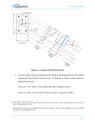
[Slenderness: Beams]
This section contains 8 lines. Each line describes a beam.
Line 1: X-Beam (perpendicular to X), Above Left
Line 2: X-Beam (perpendicular to X), Above Right
Line 3: X-Beam (perpendicular to X), Below Left
Line 4: X-Beam (perpendicular to X), Below Right
Line 5: Y-Beam (perpendicular to Y), Above Left
Line 6: Y-Beam (perpendicular to Y), Above Right
Line 7: Y-Beam (perpendicular to Y), Below Left
Line 8: Y-Beam (perpendicular to Y), Below Right
There are 7 values separated by commas for each beam in each line. (X-Beams and Y-Beams in
Slenderness dialog | Beams) These values are described below in the order they appear from left to
right.
1. 0-Rectangular Beam specified; 1-No beam specified; 2-Rigid beam specified
2. Beam span length (c/c)
3. Beam width
4. Beam depth
5. Beam section moment of inertia
6. Concrete compressive strength, f’c
7. Concrete modulus of elasticity, Ec](https://image.slidesharecdn.com/spcolumn-manual-240518140157-ee4e4ec0/85/spColumn-Manual-design-column-by-spcolumn-software-pdf-198-320.jpg)
![APPENDIX
| 199 |
[EI]
Reserved. Do not edit.
[SldOptFact]
There is 1 value in this section for slenderness factors. (Code Default and User Defined radio
buttons in Slenderness dialog | Properties | Slenderness Factors)
Code default; 1-User defined
[Phi_Delta]
There is 1 value in this section for slenderness factors. (Stiffness reduction factor in Slenderness
dialog | Properties | Slenderness Factors)
Stiffness reduction factor
[Cracked I]
There are 2 values separated by commas in one line in this section. These values are described
below in the order they appear from left to right. (Beams and Columns Cracked Section
Coefficients in Slenderness dialog | Properties | Slenderness Factors)
1. Beam cracked section coefficient
2. Column cracked section coefficient](https://image.slidesharecdn.com/spcolumn-manual-240518140157-ee4e4ec0/85/spColumn-Manual-design-column-by-spcolumn-software-pdf-199-320.jpg)
![APPENDIX
| 200 |
[Service Loads]
This section describes defined service loads. (Service Loads in Loads dialog | Loads) The first line
contains the number of service loads. Each of the following lines contains values for one service
load.
There are 25 values for each service load in one Line separated by commas. These values are
described below in the order they appear from left to right.
1. Dead Axial Load
2. Dead X-moment at top
3. Dead X-moment at bottom
4. Dead Y-moment at top
5. Dead Y-moment at bottom
6. Live Axial Load
7. Live X-moment at top
8. Live X-moment at bottom
9. Live Y-moment at top
10. Live Y-moment at bottom
11. Wind Axial Load
12. Wind X-moment at top
13. Wind X-moment at bottom
14. Wind Y-moment at top
15. Wind Y-moment at bottom](https://image.slidesharecdn.com/spcolumn-manual-240518140157-ee4e4ec0/85/spColumn-Manual-design-column-by-spcolumn-software-pdf-200-320.jpg)
![APPENDIX
| 201 |
16. EQ. Axial Load
17. EQ. X-moment at top
18. EQ. X-moment at bottom
19. EQ. Y-moment at top
20. EQ. Y-moment at bottom
21. Snow Axial Load
22. Snow X-moment at top
23. Snow X-moment at bottom
24. Snow Y-moment at top
25. Snow Y-moment at bottom
[Load Combinations]
This section describes defined load combinations. (Lod combinations in Definitions dialog | Load
Case/Combo) The first line contains the number of load combinations. Each of the following lines
contains load factors for one load combination.
Number of load combinations, n
Dead_1, Live_1, Wind_1, E.Q._1, Snow_1
Dead_2, Live_2, Wind_2, E.Q._2, Snow_2
...
Dead_n, Live_n, Wind_n, E.Q._n, Snow_n](https://image.slidesharecdn.com/spcolumn-manual-240518140157-ee4e4ec0/85/spColumn-Manual-design-column-by-spcolumn-software-pdf-201-320.jpg)
![APPENDIX
| 202 |
[BarGroupType]
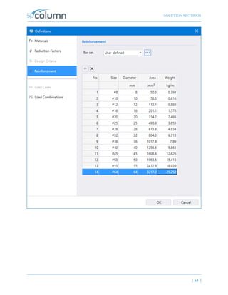
There is 1 value in this section. (Bar Set drop-down list on menu Options | Reinforcement…)
0-User Defined
1. ASTM615
2. CSA G30.18
3. prEN 10080
4. ASTM615M
[User Defined Bars]
This section contains user-defined reinforcing bars. (Bar set in Project left panel | General) The
first line contains the number of defined bars. Each of the following lines contains values for one
bar separated by commas.
Number of user-defined bars, n
Bar_1_size, Bar_1_diameter, Bar_1_area, Bar_1_weight
Bar_2_size, Bar_2_diameter, Bar_2_area, Bar_2_weight
...
Bar_n_size, Bar_n_diameter, Bar_n_area, Bar_n_weight
[Sustained Load Factors]
There are 5 values separated by commas in one line in this section. Each value respectively
represents percentage of Dead, Live, Wind, EQ, and Snow load case that is considered sustained
(Load Cases in Definitions dialog | Load Case/Combo.).](https://image.slidesharecdn.com/spcolumn-manual-240518140157-ee4e4ec0/85/spColumn-Manual-design-column-by-spcolumn-software-pdf-202-320.jpg)