1. LECTURES FOR WEEK 11
Stratified Random Sampling:
So far, we have discussed random and systematic location of cruise plots in the context of simple
random sampling. These methods work well when the area sampled is homogeneous. Foresters,
however, often cruise areas with different forest cover types (i.e., stands). These different stands
make the area heterogeneous in terms of cover types. In this case, stratified random sampling
can be used to calculate a more precise cruise.
In stratified random sampling, the units of the population (e.g., stands) are grouped together
based on similar criterion (e.g., overstory tree type). Each unit (stratum) or stand is then cruised
and the stratum estimates are combined to give an estimate for the entire area. We will illustrate
this methodology with an example.
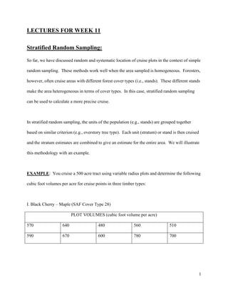
EXAMPLE: You cruise a 500 acre tract using variable radius plots and determine the following
cubic foot volumes per acre for cruise points in three timber types:
I. Black Cherry – Maple (SAF Cover Type 28)
PLOT VOLUMES (cubic foot volume per acre)
570 640 480 560 510
590 670 600 780 700
1

2. II. Yellow-Poplar – White Oak – Northern Red Oak (SAF Cover Type 59)
PLOT VOLUMES (cubic foot volume per acre)
520 710 770 840 630
760 890 810 580 860
III. White Oak – Black Oak – Northern Red Oak (SAF Cover Type 52)
PLOT VOLUMES (cubic foot volume per acre)
200 420 210 290 350
540 180 260 320 270
Mean: First, calculate the mean cubic foot volume per acre (CFV/A) for each stratum using the
simple random procedure we used earlier:
X I = 6100 / 10 = 610 cfv/a
X II = 7370 / 10 = 737 cfv/a
X III = 3040 / 10 = 304 cfv/a
The mean of the stratified sample can now be computed by:
L
∑N h ∗ Xh
X ST = h =1
,
N
where: L = The number of strata
Nh = The size of stratum h (h = 1, 2, …, L) in acres.
L
N = The total size of the tract in acres ( N = ∑ N h ).
h =1
2

3. If the strata sizes are:
NI = 250 acres
NII = 100 acres
NIII = 150 acres
Total Acres: N = 500 acres.
Then the stratified sample mean cubic volume per acre is:
250 *610 + 100 * 737 + 150 * 304
X ST = = 543.6 cfv/a
500
If you used the simple random sampling formula to calculate the mean, you would get:
16,510
XS = = 550.3 cfv/a
30
which is close to the stratified mean.
Standard Errors: Next, calculate the variance ( s 2 ) of cubic foot volume per acre (CFV/A) for
each stratum using the simple random methodology we used earlier:
s 2 = 8111.1 cfv/a
I
s 2 = 15,556.7 cfv/a
II
s 2 = 12,204.4 cfv/a
III
With these variances, calculate the stratified standard error of cubic foot volume per acre for the
sample by:
L
⎛ sh ⎞
SE ST = ∑⎜w
⎜
2
h ∗ ⎟,
⎟
h =1 ⎝ nh ⎠
where nh = number of cruise plots
wh = weight factor = Nh / N.
3

4. So, the stratified standard error for this example is:
2 2 2
⎛ 250 ⎞ 8111.1 ⎛ 100 ⎞ 15,556.7 ⎛ 150 ⎞ 12,204.4
SE SR = ⎜ ⎟ ∗ +⎜ ⎟ ∗ +⎜ ⎟ ∗ = 19.4 cfv/a ,
⎝ 500 ⎠ 10 ⎝ 500 ⎠ 10 ⎝ 500 ⎠ 10
If you used the simple random sampling formula to calculate the standard error, you would get:
SES = 38.9 cfv/a,
which is greater than the stratified standard error. Thus, stratifying the sample will improve our
overall cruise precision in this example (why?).
95% Confidence Interval: Calculate the 95% confidence interval for cubic foot volume per
acre:
X ST ± t0.05,n-1=29 * SEST ⇒ 543.6 ± 2.045*19.4 or 543.6 ± 39.7 cfv/a
Cruise Precision: Calculate the cruise precision for this stratified cruise:
SE ST * t 0.05, 29 19.4 ∗ 2.045
Pr ecision = = ∗ 100 ≅ 7%
X ST 543.6
Pr ecision (SRS) ≅ 15%
Sample Size: You can calculate the number of plots needed in each stratum that are necessary to
achieve a specified statistical objective. First, determine the total number of plots necessary by:
2
⎛ L ⎞
t * ⎜ ∑ w h * s xh ⎟
2
n= ⎝ h =1 ⎠ ,
E2
4

5. where: E = allowable error in absolute units
all other variables defined as before.
So, for our example, we want to find the number of plots needed to be 95% confident that we are
within plus or minus 10% of the true cubic foot volume per acre. In absolute units, E = 543.6
cfv/a * (0.10) = 54.4 cfv/a.
2
⎛ 250 100 150 ⎞
22 * ⎜ * 8111.1 + * 15,556.7 + * 12,204.4 ⎟
n= ⎝ 500 500 500 ⎠ ≅ 15 plots
2
54.4
For our example, we actually collected more sample points than necessary to achieve this
statistical objective.
Continuing with our example, we can now allocate (i.e., optimum allocation) these 15 plots to
the three strata with the formula:
w h * s xh
nh = L
*n
∑w
h =1
h * s xh
So,
⎛ 250 ⎞
⎜ ⎟ * 8111.1
nI = ⎝ 500 ⎠ * 15 =
45.03
* 15 ≅ 7 plots
⎛ 250 ⎞ ⎛ 100 ⎞ ⎛ 150 ⎞ 103.12
⎜ ⎟ * 8111.1 + ⎜ ⎟ * 15,556.7 + ⎜ ⎟ * 12,204.4
⎝ 500 ⎠ ⎝ 500 ⎠ ⎝ 500 ⎠
⎛ 100 ⎞
⎜ ⎟ * 15,556.7
n II = ⎝ 500 ⎠ *15 ≅ 4 plots
103.12
5

6. ⎛ 150 ⎞
⎜ ⎟ * 12,204.4
n III = ⎝ 500 ⎠ * 15 ≅ 5 plots
103.12
You will notice that the total number of plots equals 16 if you add up the strata plot numbers.
This number is greater than 15 because you should always round up the result when calculating
sample size.
You should also know that if you had an estimate of variability and you defined your strata
before the cruise, you can calculate your sample size before the cruise and allocate the plots to
each stratum with the same methodology.
6