This document presents an analysis of the relationship between Walmart stock growth and various national economic indicators over time. It examines monthly stock returns for Walmart against factors like unemployment rates, inflation rates, and various stock market indices. Regression models will be used to analyze what relationships exist between the economic variables and Walmart's performance. The analysis will provide insight into how well Walmart's business is correlated with the overall health of the economy.

1. ANALYSIS OF
WALMART
STOCK GROWTH
ABSTRACT
Analysis of Walmart Stock growth with national
economic indicators.
Lisa Feder
STA 9700- Regression Analysis

2. 1 | P a g e
Table of Contents
Chapter 1 Overview........................................................................................................................ 3
1. Topic ....................................................................................................................................... 3
2. Data Source............................................................................................................................. 3
3. Variables ................................................................................................................................. 3
4. Data View ............................................................................................................................... 3
Chapter 2 A Simple Regression Model .......................................................................................... 5
1. Scatterplots.............................................................................................................................. 5
2. Analysis of Scatterplot............................................................................................................ 5
3. The Linear Regression Model................................................................................................. 6
(a) Mean of Yx................................................................................................................... 6
(b) Terms on Right Side of E(Yx) Equation ...................................................................... 6
(c) Terms on Right Side of V(Yx) Equation...................................................................... 6
4. SAS Output for the Fitted Model............................................................................................ 6
5. Analysis of Output................................................................................................................. 7
(a) The T-Tests........................................................................................................................ 8
(b) The y -equation................................................................................................................. 8
(c) 95% Confidence and Predication Intervals ....................................................................... 8
Chapter 3. The Matrix Approach to Regression ............................................................................. 9
1. Simple Linear Regression in Matrix Terms............................................................................ 9
(a) X Matrix ....................................................................................................................... 9
(b) Y-Vector..................................................................................................................... 10
(c) Hat Matrix................................................................................................................... 10
(d) Comparison of H Matrix Excel and SAS ................................................................... 11
(e) Hat Matrix Computed Directly................................................................................... 12
2. Multiple Linear Regression in Matrix Terms ....................................................................... 12
(a) X Matrix with Two Variables.......................................................................................... 12
(b) H Matrix with Proc IML............................................................................................. 13
Chapter 4. Polynomial Regression................................................................................................ 14
1. Simple Polynomial Regression............................................................................................. 14
(a) SAS Data Program...................................................................................................... 14
(b) SAS Regression Output.............................................................................................. 14
(c) RStudent Diagnostic................................................................................................... 15
(d) Leverage Points .......................................................................................................... 16

3. 2 | P a g e
(e) T- tests and F-test for our the variables in our polynomial model ............................. 16
(f) Scatter Plots of polynomials of degree 1, 3, 4 and 10. ............................................... 17
(g) Scatter Plot Analysis................................................................................................... 19
2. Multiple Regression with a Dummy Variable and an Interaction Term............................... 19
(a) Dummy Variable Data..................................................................................................... 19
(b) Interaction Term Data ..................................................................................................... 20
(c) Regression on Interaction Term ...................................................................................... 20
(d) Dummy Variable Discussion...................................................................................... 22
(e) Interaction Term Discussion....................................................................................... 22
Chapter 5 Model Selection............................................................................................................ 22
1. Best Subsets Model Selection............................................................................................... 22
(a) Matrix Scatter Plot......................................................................................................... 22
(b) Transformation ........................................................................................................... 23
(c) Criteria Plot and Summary Table ............................................................................... 23
(d) Select Model............................................................................................................... 23
(e) Diagnostic Plots on Selected Model........................................................................... 24
2. Forward Stepwise Model Selection ...................................................................................... 26
(a) Stepwise SAS Table ................................................................................................... 26
(b) Stepwise Vs. Best Selection Method.......................................................................... 26
3. Variance Inflation ................................................................................................................. 26
(a) VIF Explanation ......................................................................................................... 26
(b) SAS Output................................................................................................................. 26
4. The Press Residuals .............................................................................................................. 27
(a) Proc Reg Vs. Proc IML .............................................................................................. 27
(b) Proc IML- Step 4, Step 7............................................................................................ 28
5. Cook's D................................................................................................................................ 28
........................................................................................................ 28
.............................................................................................................. 28
Chapter 6 GLM Select and Cross-Validation............................................................................... 30
1. GLM Select........................................................................................................................... 30
2. Cross-Section Validation ...................................................................................................... 31

4. 3 | P a g e
Chapter 1 Overview
1. Topic
This project is to study the movement of Walmart Stock Returns and see how they do in different
economic cycles. My premise
houses will need and buy even in a down economy. In fact, the theory is that Walmart does
better in down economy
2. Data Source
Yahoo Finance: Walmart Monthly Returns
Bureau of Labor & Statistics: Monthly Unemployment Rates
US Inflation Calculator: Inflation Rate
Yahoo Finance: S&P 500 Discretionary Consumption Index
Yahoo Finance: S&P 500 Index
3. Variables
x1 ~ Monthly Percentage Change in Unemployment Rate
x2 ~ Monthly Percentage Change in Inflation Rate
x3 ~ Monthly Returns of S &P Discretionary Consumption Index
x4 ~ Monthly Returns of S&P 500 Index Fund
y ~ Monthly Walmart Stock Returns
variables that are indicators of the health of the economy and will test if these
variables have any relationship with dependent variable Walmart Stock Returns.
sample and track the relationships.
4. Data View
Date X1 X2 X3 X4 Y
8/1/2015 0 0.2 9.62 -6.26 -9

5. 4 | P a g e
7/1/2015 -0.2 0.2 -3.27 1.97 1
6/1/2015 0 0.1 -1.17 -2.1 -4
5/1/2015 -0.2 0 -0.11 1.05 -4
4/1/2015 0.1 -0.2 -1.73 0.85 -5
3/1/2015 -0.1 -0.1 2.31 -1.74 -1
2/1/2015 0 0 -8.08 5.49 -1
1/1/2015 -0.2 -0.1 1.59 -3.1 -1
12/1/2014 0.1 0.8 -1.11 -0.42 -1
11/1/2014 -0.2 1.3 -3.96 2.45 15
10/1/2014 0.1 1.7 -3.30 2.32 0
9/1/2014 -0.2 1.7 4.51 -1.55 1
8/1/2014 -0.2 1.7 -4.66 3.77 3
7/1/2014 -0.1 2 2.82 -1.51 -2
6/1/2014 0.1 2.1 -2.51 1.91 -2
5/1/2014 -0.2 2.1 -2.62 2.1 -3
4/1/2014 0.1 2 2.48 0.62 4
3/1/2014 -0.4 1.5 0.70 0.69 3
2/1/2014 -0.1 1.1 -7.44 4.31 0
1/1/2014 0.1 1.6 8.71 -3.56 -5
12/1/2013 -0.1 1.5 -2.07 2.36 -2
11/1/2013 -0.3 1.2 -2.50 2.8 6
10/1/2013 -0.2 1 -3.79 4.46 4
9/1/2013 0 1.2 -5.15 2.97 1
8/1/2013 0 1.5 4.00 -3.13 -6
7/1/2013 -0.1 1.2 -5.80 4.95 5
6/1/2013 -0.2 1.8 -0.86 -1.5 0
5/1/2013 0 1.4 -3.56 2.08 -3
4/1/2013 -0.1 1.1 -3.12 1.81 4
3/1/2013 0.1 1.5 -3.23 3.6 6
2/1/2013 -0.2 2 -0.97 1.11 1
1/1/2013 -0.3 1.6 -3.85 5.04 3
12/1/2012 0.1 1.7 -2.88 0.71 -5
11/1/2012 0.2 1.8 -1.16 0.28 -4
10/1/2012 -0.1 2.2 0.39 -1.98 2
9/1/2012 0 2 -3.18 2.42 2
8/1/2012 -0.2 1.7 -4.37 1.98 -2
7/1/2012 -0.2 1.4 1.28 1.26 7
6/1/2012 0 1.7 -5.18 3.96 6
5/1/2012 0 1.7 10.22 -6.27 12
4/1/2012 0 2.3 -1.47 -0.75 -4
3/1/2012 0 2.7 -3.83 3.13 4

6. 14 | P a g e
Chapter 4. Polynomial Regression
Many times are data does not conform to a simple regression model, so we us different
techniques to see if our x and y polynomial relationship rather than linear.
1. Simple Polynomial Regression
Below we begin with simple regression using only one variable, we will select an x variable and
I used my x3 variable, the Monthly Stock Return
on the S&P 500 Discretionary Consumption Index.
(a) SAS Data Program
The program below is written to square the value of are x3 variable, then regress y on both x3
and x3
2
.
proc import datafile='C:UsersLisaDesktopLisaStat ProgramSTA 9700ProjectStock_Prices.xlsx'
dbms=xlsx out=walmart replace;
getnames=yes; sheet=Final_data;
run;
Data Poly_Reg;
Set Walmart;
x3_sqr= SP_500_Discretionary_x3**2;
run;
proc reg;
model Walmart_Stock_Prices_y = x3_sqr SP_500_Discretionary_x3;
run;
(b)SAS Regression Output
T-value: S&P 500 Discretionary
Consumption Index x3 = .0879

7. 15 | P a g e
P-value x3
2
= .2040
(c) RStudent Diagnostic
In the RStudent Diagnostic we found one point of leverage in this data this point is extreme
in the x direction in comparison to the rest of the points.

8. 16 | P a g e
(d)Leverage Points
These leverage points are computed on the diagonal of the H matrix that is used to compute the
bi -vector (slopes for the all the repressors), and by extension the y vector.
(e) T- tests and F-test for our the variables in our polynomial model
T-Test for x3 variable, (Monthly Stock Return on S&P 500 Discretionary Consumption Index)
Hypothesis Test:
H0: 1=0
H1: 1
Test statistic: t-stat =
SSxs/
0b1
= (-.2483-0)/(.14281) = -1.74 .
Rejection region: |-1.74| < 2.92
t-critical value with d.f. = 2 .
Conclusion: null hypothesis is not rejected.
Because the |t-stat| = |-1.74| less than the t-critical value of 2.92 .
T-Test for x3 variable, (Monthly Stock Return on S&P 500 Discretionary Consumption Index- Squared)
Hypothesis Test:
H0: 1=0
H1: 1
Test statistic: t-stat =
SSxs/
0b1
= (.0288)/(.02239) = 1.29 .
t-critical value with . d.f. = 2 .

9. 17 | P a g e
Conclusion: null hypothesis is not rejected.
Because the |t-stat| = |1.29| less than the t-critical value of . 2.92 .
F-test below are x3 and x3
2
H0: 1= 2 = 0 [Note that 0 is not included.]
H1: j t least one value of j
Test statistic: F-stat =
p)-SSE/(n
1)SSR/(p
= (81.278/2) / (1092.15051/53) =1.97 [p=k+1=2+1, here]
Rejection region: F-stat > F-critical value, 2 d.f., 53 d.f.,
Conclusion: the null hypothesis is not rejected.
because the F-stat of 1.97 less than the F-critical value of. 3.96 .
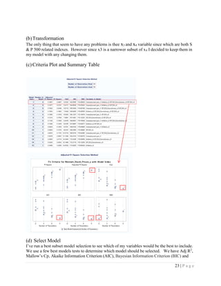
(f) Scatter Plots of polynomials of degree 1, 3, 4 and 10.
Now we will try on plot our simple regression on a polynomial of different degrees to see if our
data will fit betters with a different degree of polynomials.
model so we can compare the other higher polynomial graphs with it.
Our second plot is of degree=3, which y is regressed on x, x2
, x3
. Our objective is to see if our data fits better.

10. 18 | P a g e
Now we have a polynomial of degree=4, y regressed on x, x2
, x3
, x4
.
The last model is a polynomial of degree=10, y regressed x, x2
, x3
,x4
, x5
, x6
, x7
, x8
, x9
, x10
.
could potentially with an extreme high order model.

11. 22 | P a g e
(d)Dummy Variable Discussion
The way the dummy variable works is that it will categorize the data into the categories that was
set forth but the dummy variables (in our case high (above 3.2) and low (below 3.2) inflation
rate). It will create two y lines with the same slope but different y-intercepts.
(e) Interaction Term Discussion
The interaction variable works as a new regressor, but this term in not have linear relationship
with y. Since we are multiplying two regressors we now have a quadratic relationship.
Chapter 5 Model Selection
1. Best Subsets Model Selection
Now we going to analyze what would be the best model to use. Here we will explore if the
regressor we have our correct for our data or if some should be left out. We will also see if there
are any transformation that we can do to our data, so that it has a better linear relationship.
(a) Matrix Scatter Plot
Below is scatterplot of the full data, all the x variables and the y variable. Below we plot each
of the four regressors, against our y variable (Walmart Stock Return) and each other. We want
to see if there is multicollinearity between any of the regressors. Below we see that there is
some correlation between our x3 (S&P 500 Discretionary Consumer Index) and x4 (S&P 500
Index fund).

12. 23 | P a g e
(b)Transformation
The only thing that seem to have any problems is thee x3 and x4 variable since which are both S
& P 500 related indexes. However since x3 is a narrower subset of x4 I decided to keep them in
my model with any changing them.
(c) Criteria Plot and Summary Table
(d) Select Model
We use a few best models tests to determine which model should be selected. We have Adj R2
,
riterion (AIC), Bayesian Information Criterion (BIC) and

13. 24 | P a g e
Schwarz Criterion (SBC). Here almost all the methods choose Model One which says to
include all the variables. The only one that disagrees in SBC which says to take model Ten, that
which only includes our x4 variable.
(e) Diagnostic Plots on Selected Model
Below are the diagnostic plots and the model that was selected with all the four selected
variables.
e blown up the RStudent and to get a better look it. It shows the leverage points and outliners
in the data. Again, as discussed in an earlier section, a leverage point is an extreme point in the x
direction, an outlier is an extreme point in the y direction and an influential point is a
combination of the two.

14. 25 | P a g e
Red- Outlier
Green- Leverage Point
Orange- Leverage Point & Outlier (Influential Point)
kept the leverage points and outliers in my data to cast a broader net for the values. Since
comparison these points would be leverage points. In that way by keeping the leverage points I
can use it to help forecast other values that may vary from the data.
Below is the analysis of variance. With all of these variable only our x4 has remained
statistically significant. But our adj R2
is higher at .1436, than our original .0923 when we only
had the first two variables in our model.

15. 26 | P a g e
2. Forward Stepwise Model Selection
(a) Stepwise SAS Table
Below is the Stepwise selection method. What this does is that it start by bringing in the variable
with the Partial R-Square and then one by one determines if the additional variables should be
added. If also will drop earlier variables along the way if it is necessary. In our case The
Stepwise Model brought in all the variables.
(b)Stepwise Vs. Best Selection Method
The results from the stepwise method match what we got in the best subsets method they both
leave all variables in the model.
3. Variance Inflation
(a) VIF Explanation
VIF shows if there is any correlation between the variables. The formula is 1/(1-Rk
2
) so that if
the correlation is low VIF will be close to 1 and if correlation is high correlation the VIF will
be large. Then we would take one of the variables out of the model. Large values of VIF and
high correlation of variables tend to increase the variance of the slopes. In our data there are
no extreme values of VIF.
(b)SAS Output
Below is the regression that was run including the VIF information. None of the values
are extremely high which suggest that none of the variables are too closely related and
have different attributes to contribute to the model.