This document is a thesis that evaluates investment strategies. It first reviews literature on performance evaluation measures. It then defines and describes various return, risk, return-to-risk, benchmark, and other quantifiable measures to evaluate past investment performance. It discusses potential misuses of these measures and stresses the importance of evaluating measures together. It also covers non-quantifiable evaluation criteria. Finally, it applies the discussed performance measures and principles to evaluate the past 10 years of Slovak equity pension funds.

1. COMENIUS UNIVERSITY BRATISLAVA
FACULTY OF MATHEMATICS, PHYSICS AND INFORMATICS
Evaluation of Investment Strategies
RIGOROUS THESIS
Bratislava 2016 Msc. Igor Vilcek

2. COMENIUS UNIVERSITY BRATISLAVA
FACULTY OF MATHEMATICS, PHYSICS AND INFORMATICS
Department of applied mathematics and statistics
Evaluation of Investment Strategies
RIGOROUS THESIS
Study programme: Economic and Financial Mathematics
Field of study: 9.1.9 Applied Mathematics, 1114
Department: Department of Applied Mathematics and Statistics
Bratislava 2016 Msc. Igor Vilcek

3. Abstract
VIL ˇCEK, Igor: Evaluation of investment strategies [rigorous thesis]. Comenius Univer-
sity, Bratislava. Faculty of Mathematics, Physics and Informatics. Department of App-
lied Mathematics and Statistics. Bratislava: FMFI UK, 2016. 89 pages.
The paper is focused on an ex-post investment performance analysis. Firstly, we create
a suite of return, risk, return to risk and benchmark related measures with immediate
real life applications in mind. We define and describe these measures and provide real
data examples where appropriate. Secondly, we take a look at common mistakes per-
formed by practitioners. For each measure, we assess potential misuses and potential
misinterpretations of conclusions resulting from them. We also include the visual ana-
lysis. Moreover, we analyze advantages and disadvantages of specific measures and
show how to use them appropriately. We furthermore stress that it is necessary to eva-
luate measures in conjunction with each other. We complement the analysis by brief
discussion of non-quantifiable, more qualitative, criteria. Lastly, in the practical sec-
tion, we apply all performance measures and discussed principles in evaluation of the
ten years of historical data of the Slovak equity pension funds in the funded pillar.
Keywords: performance evaluation, investment performance measurement, port-
folio performance, fund performance analysis, risk-return analysis, the funded pillar
of the Slovak pension system.

4. Table of Contents
Introduction 1
1 Literature 4
2 Ex-post evaluation 6
2.1 Return measures . . . . . . . . . . . . . . . . . . . . . . . . . . . . . . . . 8
2.1.1 Visual inspection . . . . . . . . . . . . . . . . . . . . . . . . . . . . 9
2.1.2 Cumulative annual growth of return . . . . . . . . . . . . . . . . . 15
2.1.3 Rolling return . . . . . . . . . . . . . . . . . . . . . . . . . . . . . . 15
2.1.4 Calendar returns . . . . . . . . . . . . . . . . . . . . . . . . . . . . 16
2.1.5 Distribution of returns . . . . . . . . . . . . . . . . . . . . . . . . . 16
2.2 Risk measures . . . . . . . . . . . . . . . . . . . . . . . . . . . . . . . . . . 17
2.2.1 Volatility . . . . . . . . . . . . . . . . . . . . . . . . . . . . . . . . . 18
2.2.2 Maximum drawdown . . . . . . . . . . . . . . . . . . . . . . . . . 21
2.2.3 Time to recovery . . . . . . . . . . . . . . . . . . . . . . . . . . . . 24
2.2.4 Value at risk . . . . . . . . . . . . . . . . . . . . . . . . . . . . . . . 25
2.3 Return to risk measures . . . . . . . . . . . . . . . . . . . . . . . . . . . . 26
2.3.1 Sharpe ratio . . . . . . . . . . . . . . . . . . . . . . . . . . . . . . . 26
2.3.2 Sortino ratio . . . . . . . . . . . . . . . . . . . . . . . . . . . . . . . 28
2.3.3 DVR ratio . . . . . . . . . . . . . . . . . . . . . . . . . . . . . . . . 29
2.3.4 Calmar ratio . . . . . . . . . . . . . . . . . . . . . . . . . . . . . . . 30
2.3.5 CAR to Xth percentile of drawdown . . . . . . . . . . . . . . . . . 31
2.3.6 Omega ratio . . . . . . . . . . . . . . . . . . . . . . . . . . . . . . . 31
2.3.7 Return to maximal loss . . . . . . . . . . . . . . . . . . . . . . . . . 32
2.3.8 Ulcer performance index . . . . . . . . . . . . . . . . . . . . . . . 33
2.4 Other quantifiable measures . . . . . . . . . . . . . . . . . . . . . . . . . . 33
2.4.1 Statistical significance . . . . . . . . . . . . . . . . . . . . . . . . . 33
2.4.2 Skewness . . . . . . . . . . . . . . . . . . . . . . . . . . . . . . . . 35
2.4.3 Kurtosis . . . . . . . . . . . . . . . . . . . . . . . . . . . . . . . . . 36
2.4.4 Fractal efficiency . . . . . . . . . . . . . . . . . . . . . . . . . . . . 37
2.4.5 K-ratio . . . . . . . . . . . . . . . . . . . . . . . . . . . . . . . . . . 38
2.5 Benchmark related measures . . . . . . . . . . . . . . . . . . . . . . . . . 39
2.5.1 Jensen’s alpha . . . . . . . . . . . . . . . . . . . . . . . . . . . . . . 40

5. 2.5.2 Black-Treynor ratio . . . . . . . . . . . . . . . . . . . . . . . . . . . 41
2.5.3 Tracking error . . . . . . . . . . . . . . . . . . . . . . . . . . . . . . 42
2.5.4 Information ratio . . . . . . . . . . . . . . . . . . . . . . . . . . . . 42
2.5.5 Treynor ratio . . . . . . . . . . . . . . . . . . . . . . . . . . . . . . 43
2.6 Criteria difficult to measure . . . . . . . . . . . . . . . . . . . . . . . . . . 43
2.6.1 Reputation of the manager . . . . . . . . . . . . . . . . . . . . . . 44
2.6.2 Credit risk . . . . . . . . . . . . . . . . . . . . . . . . . . . . . . . . 44
2.6.3 Liquidity risk . . . . . . . . . . . . . . . . . . . . . . . . . . . . . . 44
2.6.4 Pricing risk . . . . . . . . . . . . . . . . . . . . . . . . . . . . . . . 45
2.6.5 Market risk . . . . . . . . . . . . . . . . . . . . . . . . . . . . . . . 45
2.6.6 Details regarding investment strategy . . . . . . . . . . . . . . . . 47
3 The practical ex-post evaluation 49
3.1 The funded pillar of the Slovak pension system . . . . . . . . . . . . . . . 49
3.1.1 Brief history . . . . . . . . . . . . . . . . . . . . . . . . . . . . . . . 49
3.1.2 Current setup of the pillar . . . . . . . . . . . . . . . . . . . . . . . 50
3.2 Description of the measures and data . . . . . . . . . . . . . . . . . . . . 50
3.2.1 Fund data . . . . . . . . . . . . . . . . . . . . . . . . . . . . . . . . 50
3.2.2 Performance measures . . . . . . . . . . . . . . . . . . . . . . . . . 51
3.3 Evaluation . . . . . . . . . . . . . . . . . . . . . . . . . . . . . . . . . . . . 54
3.3.1 Visual Evaluation . . . . . . . . . . . . . . . . . . . . . . . . . . . . 54
3.3.2 The whole sample . . . . . . . . . . . . . . . . . . . . . . . . . . . 65
3.3.3 First part of the sample . . . . . . . . . . . . . . . . . . . . . . . . 70
3.3.4 Second part of the sample . . . . . . . . . . . . . . . . . . . . . . . 71
3.3.5 Third part of the sample . . . . . . . . . . . . . . . . . . . . . . . . 73
3.3.6 Criteria difficult to measure . . . . . . . . . . . . . . . . . . . . . . 74
Conclusion 84

6. Introduction
The number of investment products available for investors nowadays is reaching over-
whelming levels and is further growing. It is still more complicated and complex for
an investor to assess which investment product is suitable for his investment objec-
tive. For a product an investor needs to consider almost endless number of aspects
such as the future return potential, an alignment of the product against his investment
objective, investment horizon, risks associated with it, costs, threats of a potential mis-
leading marketing as well as historical performance of the same or similar products.
The last is perhaps the most easily accessible and quantifiable and represents the foun-
dation for this paper.
Many practitioners and even some investment professionals do not evaluate the
performance of investment strategies correctly. It is a very common practice to judge
an investment only by means of a price chart of an equity curve of an investment.
This, stand-alone, is not sufficient for assessment of investment’s past risk and return
characteristics. Moreover, even carrying out a so called visual inspection of the chart is
often done incorrectly by analysts. Scaling, frequency of the displayed returns or the
length of the charts is often misused and incorrectly interpreted, whether consciously
or unconsciously.
Not uncommon is putting too much emphasis on the return side of the strategy.
Practitioners very often base their investment decisions only on the past returns and
do not put enough focus on all of the risks associated with an investment. It is often
forgotten that if a specific risk event such as default is triggered, it may substantially
or even completely reduce returns on an investment. For that reason it is of uttermost
importance to focus on the return in conjunction with the risk associated and never on
the return alone.
Even in case a potential investor conducts a return to risk analysis, it may be in-
sufficient, calculated incorrectly or lacking other important return to risk measures
necessary to be taken into account. Many practitioners focus on just one or two re-
turn to risk measures. They sometimes use the annualization incorrectly or compare
investments between each other in spite of each of them being scaled differently. All
of these introduces misuse of a performance evaluation.
Last but not least, it is not enough to assess only quantifiable statistics of an in-
vestment themselves. Besides them, one needs to take into account effects difficult to
1

7. 2
measure such as liquidity, credit quality, currency risk or details regarding investment
strategy. It is worth mentioning that these may often only be obtainable from detailed
reports or in the worst case only by means of contacting the investment manager.
This paper attempts to address most of the above mentioned issues. We focus on
an ex-post investment performance analysis. This analysis is purely based on the his-
torical price data and does not cover predictions of a future performance, fundamental
analysis or analysis of single trades. We thus do not focus on an ex-ante evaluation of
a potential strategies but rather on an analysis of existing strategies with long enough
track record. Nonetheless, we are aware of the fact that an ex-post analysis of the his-
torical data is not fully sufficient to completely assess a suitability of an investment.
Ex-ante analysis, however, is beyond the scope of this paper.
As we are not aware of the relevant literature which describes the ex-post per-
formance measures, provides real data examples, discusses their pros and cons, the
common misuses of the measures and which applies the measures again to the real
data, we aim to accomplish this.
We will focus on an evaluation of the strategies as such, rather than compared to
some benchmark. The reason is twofold. Firstly, most of the investors are usually con-
cerned about the performance of a strategy as such and not about outperformance
against some abstract benchmark. Secondly, a choice of the benchmark is often dis-
putable and not always unambiguous. Hence, the majority of the paper will be devo-
ted to the return, risk and return to risk measures which do not involve comparison
against benchmark. Nonetheless, because it is still important for many analysts to also
assess the performance against some pre-specified benchmark, we do include a sec-
tion devoted to benchmark related measures. Aim of this paper is not to cover all of
the existing measures. The aim is to describe as many different measures as possible
which do complement each other and may add value when introduced into the deci-
sion making process.
Purpose of this text is as following. Firstly we aim to create a suite of return, risk,
return to risk and benchmark related measures suitable for the immediate real life
application. We define and describe the measures and attempt to provide real data
examples where appropriate. Next, we aim to discuss the common mistakes made by
practitioners, the common misuse of the measures and a potential misinterpretation
of the resulting values of the measures. We also devote a section to the visual ana-
lysis. Moreover, we aim to discuss the advantages and disadvantages of the specific
measures and describe the cases in which it is appropriate to use a specific measure.
Furthermore, we want to stress that it is necessary to evaluate the measures in conjunc-
tion with each other rather then to arrive at conclusions based just on a single measure.
We complement the analysis by brief discussion of the criteria which are difficult to
be measured. Last but not least, we apply all of the defined measures and discussed
principles to the ten years of historical data of the Slovak equity pension funds in the

8. 3
funded pillar (defined contribution pension scheme).
The paper is organized as follows. The first chapter summarizes the relevant litera-
ture. The second chapter focuses on the entire ex-post evaluation in terms of defining
and describing the measures. First section describes the return measures and addres-
ses the visual inspection, second section the risk measures, third section the return to
risk measures, fourth section the other quantifiable measures, fifth section the bench-
mark related measures and sixth section the criteria difficult to measure. In the third
chapter we apply the measures defined and described in the second chapter to the
real data. In the first section we briefly introduce the Slovak funded pension pillar,
in the second section we describe our data and summarize the measures and in the
third section we carry out the visual as well as the quantitative (and very briefly also
qualitative) evaluation. The final chapter concludes.

9. Chapter 1
Literature
Literature analyzing an investment performance started emerging as soon as in the
1960s, see for example [1], [2] or [3]. The majority of the literature since then has been
focused on a single specific phenomenon, a new performance measure or an evalu-
ation of a specific investment segment, see for example [4], [5] or [6]. Only few of the
papers attempted to provide a more general framework or a review applicable to the
large, diverse universe of assets, for example [7]. In our paper we focus on an easy to
implement general framework for evaluation of an investment performance.
Closest to our paper in terms of content is the work of Veronique le Sourd in [8].
The paper is devoted to the performance measurement for traditional investments. It
provides a comprehensive review of performance measures with many of them invol-
ving factor models and regression analysis. It also describes models that take a step
away from modern portfolio theory and allow a consideration of cases beyond mean-
variance theory. An author starts with different methods used in the return calcula-
tion, continues with absolute and relative risk-adjusted performance measures and
also with the review of a new research on the Sharpe ratio. The second part of the
paper is devoted to the measures of risk, downside risk and to the higher moments
analysis. It also contains some more advanced models of a performance measurement
using conditional beta and methods that are not dependent on the market model. It
concludes with the factor models review. We appreciate the comprehensiveness of the
review, the mathematical exactness as well as the inclusion of many of the relevant
references to the original papers. On the other hand, the paper does not provide any
practical applications or suggestions for implementation and some of the measures
from the paper are really hard and exhausting to implement. Moreover, many of the
measures listed are very similar to each other. We also miss the discussion of the ad-
vantages and disadvantages of the measures and appropriateness of their utilization
in specific cases. Based on the aforementioned facts about the paper, we decided to
focus on simple to implement performance measures, diverse enough to complement
each other, and provide many real data examples and suggestions for implementation.
One of the classic theoretical books from the field of the portfolio analysis which
is definitely a must-read for any professional interested in the subject is the work of
4

10. CHAPTER 1. LITERATURE 5
Elton, Gruber, Brown and Goetzmann in [9]. The book devotes a section also to the
evaluation of the investment process, mutual funds and portfolio performance, but is
not primarily focused on this topic.
The very comprehensive book on the topic of quantitative finance and portfolio
analysis, which also contains many of the VBA code ready for the practical imple-
mentation, is the work of Wilmott in [10]. It may be of a high value for any reader
who is interested in more details in specific topics, such as modeling of the volatility,
mentioned also in our paper.
The more practical paper devoted to the performance evaluation has been written
by Eling in [11]. His work is focused on the comparison of the Sharpe ratio measure
with other performance measures in terms of ranking the mutual and hedge funds’
performance. Eling has analyzed a data set of 38 954 funds investing in various asset
classes. He has found that the ranking order of the funds utilizing the Sharpe ratio is
virtually identical to the ranking order generated by other performance measures used
in his paper. Eling thus argues that the Sharpe ratio is an appropriate performance me-
asure even in cases when returns of investments are not normally distributed, which
is the case for hedge funds, mutual funds and many other asset classes analyzed in his
paper.

11. Chapter 2
Ex-post evaluation
In the following chapter we will describe the most important ex-post performance
evaluation measures. As a reader may already find many of these in an existing lite-
rature, what we consider even more important, and one of the main contributions of
this paper, we present the evaluation measures along with the real world examples of
their advantages and disadvantages. We discuss what they are mainly suited for and,
on the other hand, what we cannot conclude purely by examining them.
Ex-post evaluation of an investment strategy can be interpreted as an evaluation
in case that we already know the outcome of the strategy. In other words, we already
have the real performance data of the fund employing the strategy, or at least real out
of sample results of a trading account. Ex-post evaluation of a strategy is often insight-
ful for many different types of professionals. Definitely, it is frequently being carried
out by a company managing the strategy, to have a thorough understanding of its real
world, or out of sample, performance. Next, it is naturally of uttermost importance for
existing or prospective investors in the strategy. Last but not least, many third party
evaluators, such as the regulator, researchers or journals discussing investment oppor-
tunities carry out the analysis often as well.
At first sight this evaluation process seems to be quite straightforward - we have
the data, for which we need to calculate some known descriptive statistics, evaluate
them and finally decide if we are satisfied with the observed outcome or not. As easy
as it may seem, there are however many pitfalls that an evaluator has to face. Someti-
mes even investment professionals with years of experience omit important decision
factors, neglect statistics needed to properly assess the particular strategy or oversim-
plify their analysis. We think it is crucial to consider as many performance statistics as
possible and, at least, start with an ample universe1
of potential evaluation measures.
1
We however do not aim to list every single existing evaluation criterion. Since the number of inves-
tment performance statistics can easily count into hundreds, we focus on the most important statistics
that we think are inevitable to consider at least in some specific cases. For more comprehensive and also
different list of performance measures we refer a reader for example to [8].
6

12. CHAPTER 2. EX-POST EVALUATION 7
Thereafter we may choose the most suitable subset for an investment that is to be eva-
luated.
Before proceeding to the definitions of the specific evaluation measures, it is useful
to categorize the measures into basic groups.
Firstly, it is important to be aware that the measures described below could be
calculated from two types of fund’s (or strategy’s) data. Each type has a distinct func-
tion in evaluation of the strategy. The first is a computation of the measures from the
realized returns of the whole strategy (daily, weekly or different). The second is a com-
putation of the statistics from the closed trades which the strategy has made. Each of
them produces different results and each of them is differently accessible. On the one
hand it is almost impossible to get the data of individual trades for a person not in-
volved in the management of the strategy. On the other hand, it is very easy to obtain
the daily equity curve data of a publicly listed fund, and hence its strategy returns, for
any external researcher. In this chapter we will focus on the measures computed from
the first type of data, since the majority of these measures can be easily adapted also
to the second type of data.
Secondly, a strategy can be evaluated as such, i.e. on a stand-alone basis, or with re-
gards to a chosen benchmark. The first type of assessment is more suitable for absolute
return strategies, which usually do not have a pre-specified market benchmark. The
second type of evaluation applies better to a so called „beta” strategies or „market”
strategies, i.e. investments which are in some way tied to a specific market bench-
mark. Since most of the investors are usually concerned about the performance of a
strategy as such, and not about outperformance against some abstract benchmark, we
will focus our analysis on the first type of measures, i.e. absolute return. For the sake
of integrity we add a separate category discussing measures related to a benchmark.
Last but not least, evaluation measures can describe only the return part of an in-
vestment, or only the risk attributes of an investment, or both of them. Division based
on these differences will be our chosen categorization. Basically, evaluation measures
can be divided into 5 distinct categories - return measures, risk measures, return to risk
measures, other quantifiable measures and criteria difficult to measure. As mentioned above,
most of them can be related to either calendar returns or closed trades (e.g. return dis-
tribution of the daily returns or return distribution of the trades). In this paper we will
not be analyzing the trade specific data, which is very hard to obtain, and rather focus
on historical returns. To address the issue of a comparison of an investment against the
benchmark we also add the last category which we call the benchmark related measures.

13. CHAPTER 2. EX-POST EVALUATION 8
2.1 Return measures2
Calendar days versus trading days
In every calculation we have to firstly decide whether we will use a calendar day con-
vention or a trading day convention. This can be illustrated on an example of a sample
starting on 31.12.2014 and ending on 31.12.2015. In terms of the calendar day con-
vention we have the sample of length n = 366 calendar days with t0 = 31.12.2014,
T = 31.12.2015 and hence, if we assign a serial number to each day, T − t0 = 365.
In terms of the trading day convention we have a sample of length d = 253 trading
days3
with t0 = 1 (first trading day), T = 253 (253-th trading day), T − t0 = 252 and
d − 1 = 252 return observations. We will always state what convention we are using.
Simple return
If Pt0 and PT , where T > t0 are the prices of an evaluated asset at times t0 and T
respectively, then let us define the return on an investment from (either calendar or
trading) period t0 to period T as follows
rT
t0
=
PT
Pt0
− 1. (2.1)
This is the simple arithmetic return for the whole period, or in financial jargon
also flat return, without annualization. Throughout the paper we will utilize this sim-
ple arithmetic measure of return instead of log-returns, because it exactly represents
an investor’s return on their investment, without any approximation. Log-returns of
course do have important properties when used for modeling involving normal dis-
tribution, but throughout this section we will not be modeling the aforementioned.
We will omit the superscript when dealing with just 1-tick4
returns instead of whole
period returns (such as a 1-day return instead of a 1-year return) and denote as ri only,
where ri = rt0+i
t0+i−1 , i = 1, . . . , T − t0 .
Note that, for example, r1 = rt0+1
t0
denotes return from the close of the trading (or
calendar) day 1 (that is t0) to the close of the trading (or calendar) day 2.
2
We omit the prefix „historical” from any of the following measures for the sake of readability.
3
Measured by the number of trading days on the New York stock exchange. The average number
of trading days per year on the American stock exchanges is 252.
4
The smallest tick or, in other words, the highest frequency used in this paper will be 1 day, that is
daily frequency. However, all of the measures and calculations are applicable in the same way to any
other frequency, higher or lower.

14. CHAPTER 2. EX-POST EVALUATION 9
2.1.1 Visual inspection5
Many professionals base their investment decisions on a visual inspection of the charts
of investments. This is usually just a part of the decision making process. However,
whether one admits it or not, it is still heavily used, despite all of the perils of doing
so. These include but are not limited to looking just at the historical (and not the future
potential) price evolution and many biases related to imperfections of the human jud-
gement. We do not argue against visual inspection, we, however, stress the importance
of the correct visual inspection.
Logarithmic charts
A special treatment should be applied to the very long (years or tenths of years) charts
or charts in which the securities displayed experience an exponential growth. One
of the ways how to deal with such charts is to partition the analysis to more shorter
horizons and examine each of them separately. Another way, which enables an exami-
nation of the whole chart at a time, is to use the (natural) logarithm of the time series
of the prices instead of the original time series of the prices.
Fig. 2.1: Price series of the S&P 500 price index from 3.1.1928 to 31.12.1996. Data source: Bloom-
berg
Why is this important and why may this cause problems? Consider an example in
the figure (2.1). In the figure is displayed an American equity market price index S&P
5
It is not clear whether a visual inspection should be categorized into a return, risk, return to risk or
criteria difficult to measure category. Although it most likely belongs into the last mentioned category,
we include it into the return measures category. We do so because we think it is important to address
the main issues about a visual inspection in the beginning rather than in the end of the chapter.

15. CHAPTER 2. EX-POST EVALUATION 10
500 (without dividends)6
from 1928 to 1996. Consider now an analyst trying to quickly
assess the risk of this potential investment just by examining the chart. The analyst de-
cides to do this by finding the largest peak to through losses (maximum drawdown,
see section (2.2.2)) of an index in the chart. The largest loss he is able to observe is the
crash of the index in 1987, when the index lost −33.2% from its peak to its through.
The problem with the non-logarithmic chart of such a long history is that an expo-
nential growth which an index experienced makes it almost unable to correctly ana-
lyze the periods prior to the growth. And because most of the growth occurred during
the 1980s and the 1990s, the price evolution during 1928-1980 is almost impossible
to observe. The figure (2.2) displays the natural logarithm of the prices of an index
during the same period.
Fig. 2.2: Natural logarithm of the price series of the S&P 500 price index from 3.1.1928 to
31.12.1996. Data source: Bloomberg
The figure (2.2) is much more revealing when considering price evolution during
earlier part of the history displayed. We can now much more easily see the huge losses
which an index experienced during the Great Depression in the earlier 1930s. The
maximum peak to through loss (maximum drawdown) reached −86.1% in 1932.
Frequency of the charts
For the purposes of visual inspection, we prefer as high frequency as possible. This is
also the reason why we use the daily frequency of charts and returns in most of the
examples throughout the paper. As already mentioned, our preferred frequency is the
6
S&P 500 is the most widely used American stock market index consisting of 500 largest (measured
by market capitalization) American stocks.

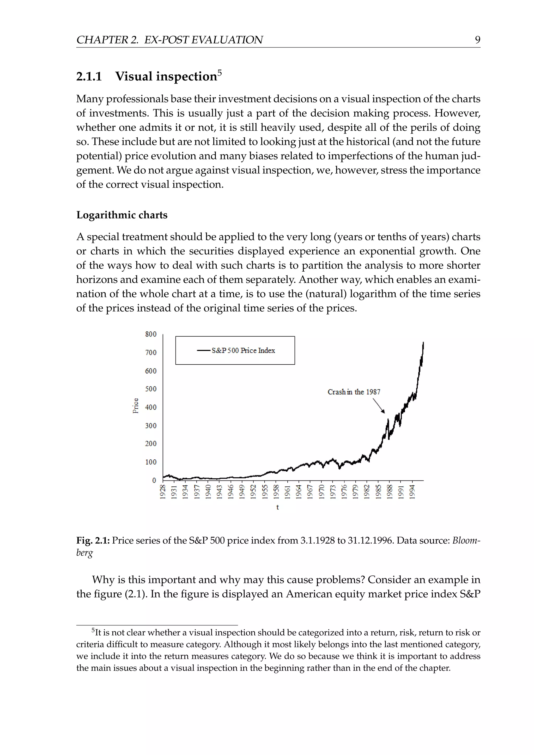
16. CHAPTER 2. EX-POST EVALUATION 11
daily frequency, contrary to some of the literature on this topic.7
Many hedge funds,
mutual funds or financial advisors report their performance on a weekly, monthly
or some even on a quarterly basis. Although the return realized on an investment is
the same regardless of the frequency of reporting chosen, the judgement of the risk
becomes highly misleading with lower frequencies. Especially drawdowns (largest
historical peak to through losses of an investment, see section (2.2.2)) but also many
other risk characteristics may be highly underestimated when measured over low fre-
quencies. Actually, in practice many funds rely on a monthly pricing of their net asset
values, because that way they may be better able to smooth the performance, hiding
the intra-month price swings.
An example of how the risk of an investment may be underestimated when using
lower frequencies can be illustrated on the American equity market index S&P 500
with net (after tax) reinvested dividends. Let us calculate the historical maximum dra-
wdown for the index (that is the maximum historical peak to through loss, see section
(2.2.2)) during the period starting on 4.1.1999 and ending on 29.2.2016. We will calcu-
late the drawdown using daily, monthly, quarterly and yearly price data of the afo-
rementioned index. The maximum drawdown when using the daily data is −55.7%,
when using monthly data −51.4%, when using quarterly data −46.4% and when using
yearly data −38.4%. The reason why the drawdown gets larger (more negative) with
higher frequency is pretty straightforward. Lower frequencies smooth the data and
therefore the sample then contains fewer price deviations. Consider also this simple
numerical illustration. Assume an index starts the month with the value of 1, in the
middle of the month falls to the value of 0.9 and ends the month by the jump back to
the value 1. Its largest monthly peak to through loss would be 0 (from 1 to 1) but its
largest daily peak to through loss would be −10%. This illustrates the importance of
using high enough frequencies to assess the risk of an investment.
Scaling
Although it should be quite obvious for everyone involved in an investment analysis,
it is still important to emphasize that different investments should be compared fairly,
on the same scale, with the same frequency and with the same (correct) adjustments
applied. This means that, firstly, the frequency of returns (and thus pricing) should be
the same for the investments under inspection.8
7
For example [8] advocates for using lower frequencies, such as monthly, because of the smaller no-
ise. They argue, firstly, that lack of synchronization of different investments over a single day may cause
problems. Secondly they argue that the common assumptions about asset returns (normal distribution,
independent, identically distributed returns) are more plausible for returns of lower frequencies. Des-
pite all of these, we prefer higher frequencies such as daily to be able to assess risk of an investment on
a daily, not only a monthly basis.
8
Common mistake in this area is to compare the volatility of the monthly returns with the volatility
of the daily returns. Even after annualization of the both aforementioned returns, they produce different

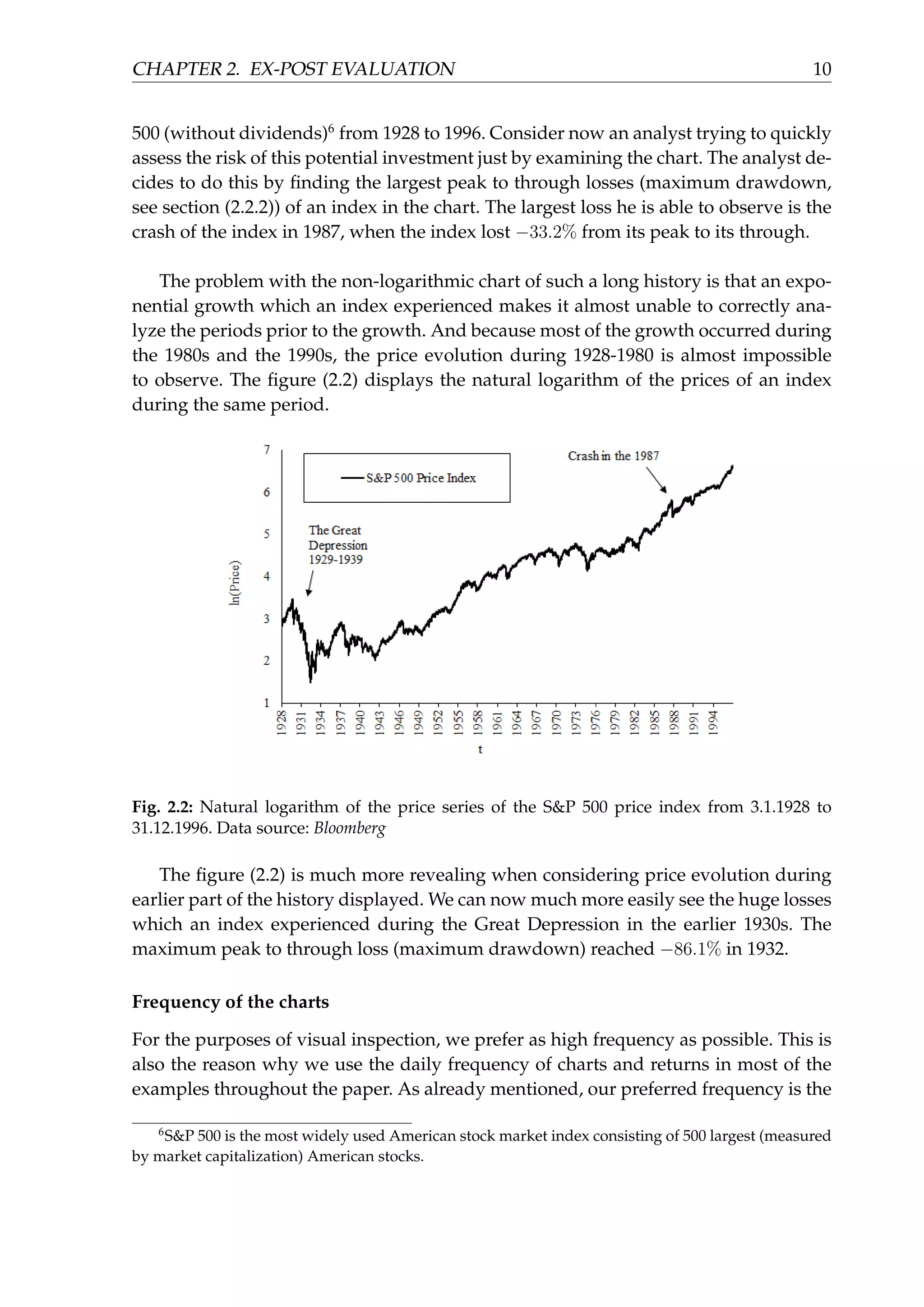
17. CHAPTER 2. EX-POST EVALUATION 12
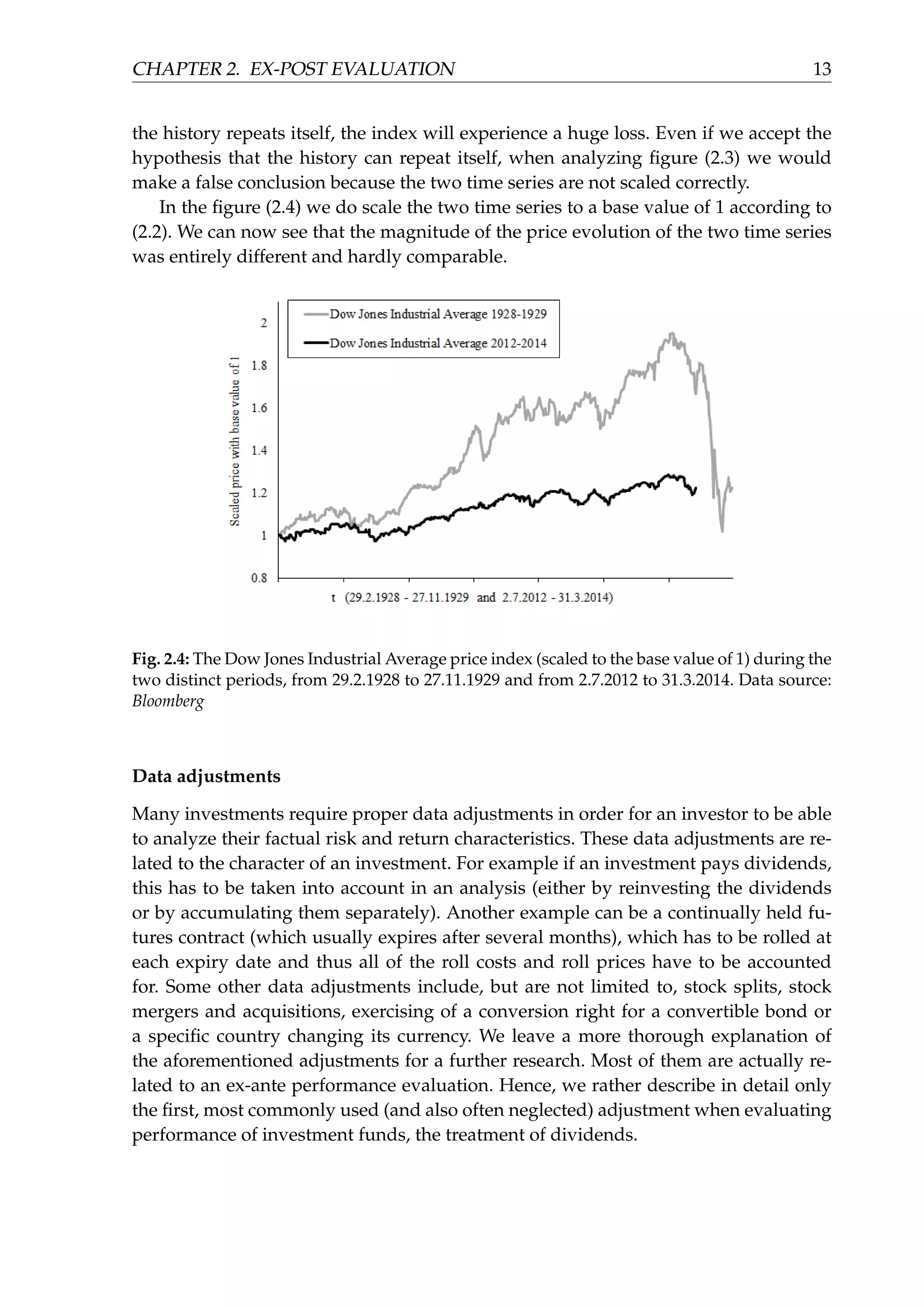
Secondly, when charted in the same figure for the purposes of comparison, it is
essential to scale the base (first) value of all charted investments to the same value.
If {Pt}T
t=t0
is the original time series of prices of an investment and { ¯Pt}T
t=t0
is the
new scaled time series with the new base value set to ¯Pt0 (most commonly ¯Pt0 = 1)
then we obtain the new scaled time series from the original one as
¯Pt = ¯Pt0 · (1 + rt
t0
) , t0 < t ≤ T , (2.2)
where rt
t0
is the flat return from (2.1).
In practice, we often witness a comparison of two different investments or a com-
parison of the current price evolution of the security with some piece of its history,
where each price is displayed on a different axis of the same figure. This highly dis-
torts the comparison, because we cannot infer if the (percentage) magnitude of the
moves in price of investments is similar or not.
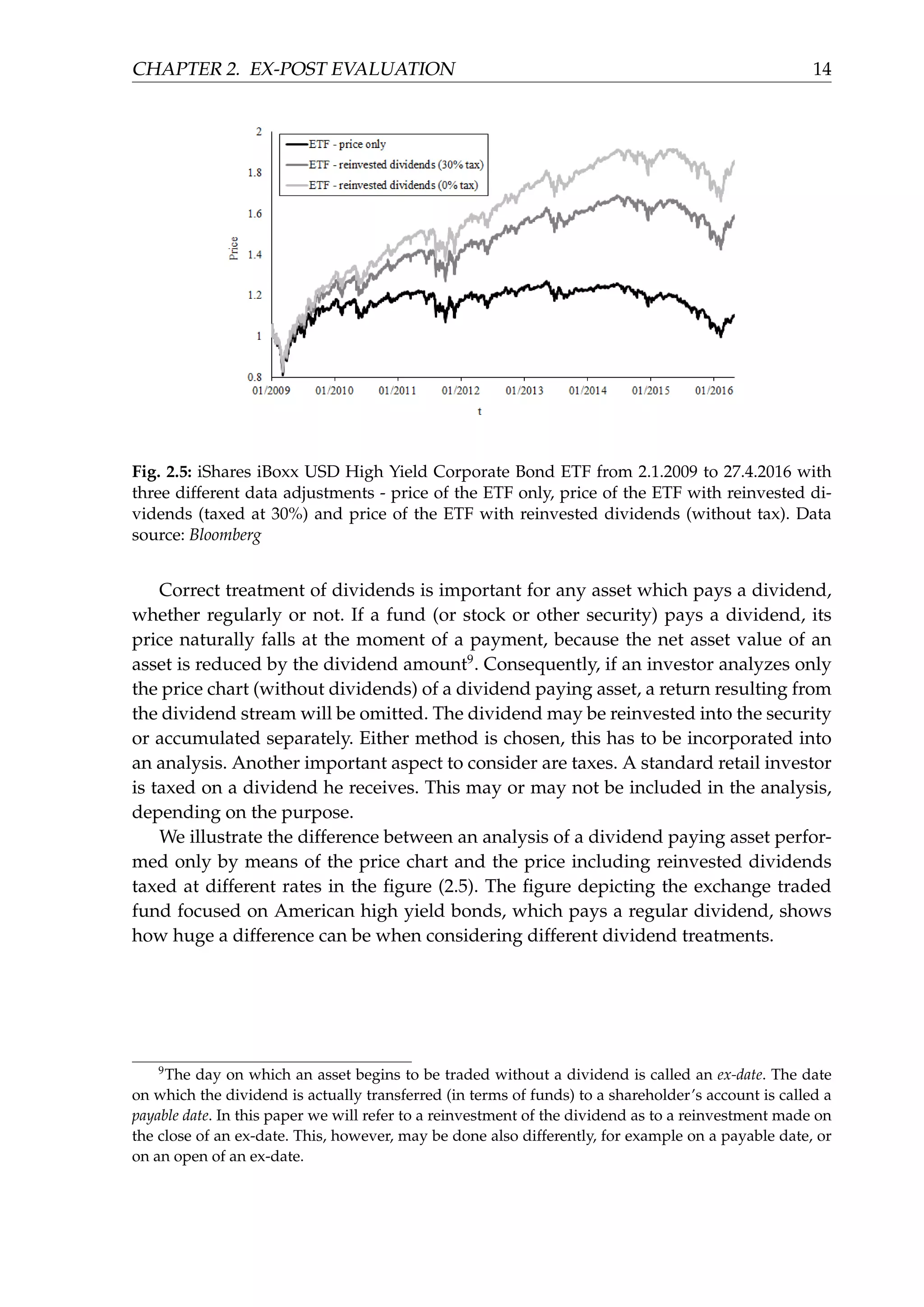
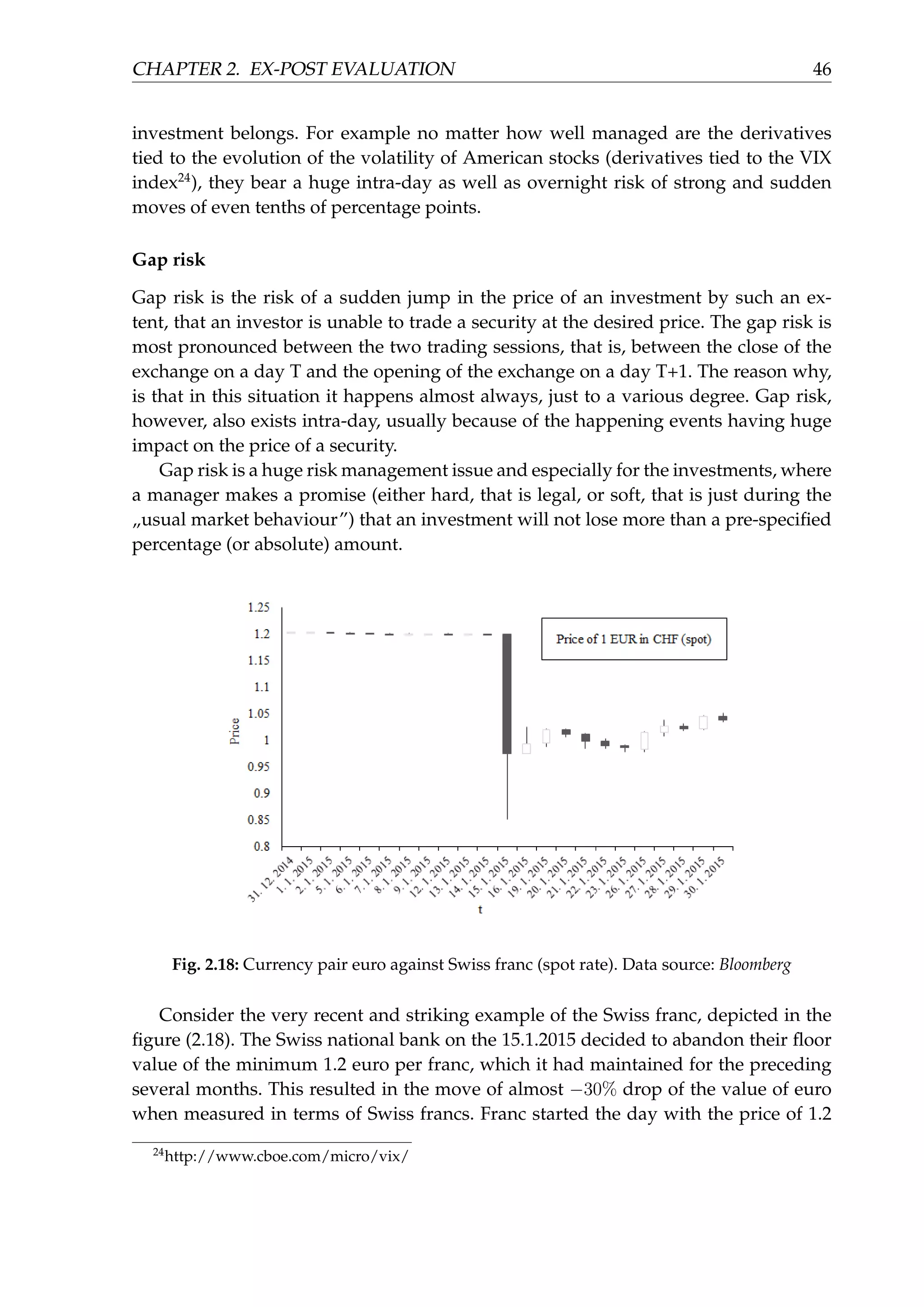
Fig. 2.3: The Dow Jones Industrial Average price index (absolute values) during the two dis-
tinct periods, from 29.2.1928 to 27.11.1929 and from 2.7.2012 to 31.3.2014. Data source: Bloom-
berg
Consider an example from the blog The Mathematical Investor [12]. As the blog
points out, in February 2014 an article appeared on a web page which is focused on
investing [13]. The article described a „scary” parallel between the price evolution of
the Dow Jones Industrial Average (American stock market price index consisting of 30
companies) from July 2012 to February 2014 and the price evolution of the same index
but from March 1928 to October 1929 (see figure (2.3)). The article suggested, that if
results. The volatility of the monthly returns will be almost always quite different from the volatility of
the daily returns. And this applies to almost any performance measure chosen.

18. CHAPTER 2. EX-POST EVALUATION 13
the history repeats itself, the index will experience a huge loss. Even if we accept the
hypothesis that the history can repeat itself, when analyzing figure (2.3) we would
make a false conclusion because the two time series are not scaled correctly.
In the figure (2.4) we do scale the two time series to a base value of 1 according to
(2.2). We can now see that the magnitude of the price evolution of the two time series
was entirely different and hardly comparable.
Fig. 2.4: The Dow Jones Industrial Average price index (scaled to the base value of 1) during the
two distinct periods, from 29.2.1928 to 27.11.1929 and from 2.7.2012 to 31.3.2014. Data source:
Bloomberg
Data adjustments
Many investments require proper data adjustments in order for an investor to be able
to analyze their factual risk and return characteristics. These data adjustments are re-
lated to the character of an investment. For example if an investment pays dividends,
this has to be taken into account in an analysis (either by reinvesting the dividends
or by accumulating them separately). Another example can be a continually held fu-
tures contract (which usually expires after several months), which has to be rolled at
each expiry date and thus all of the roll costs and roll prices have to be accounted
for. Some other data adjustments include, but are not limited to, stock splits, stock
mergers and acquisitions, exercising of a conversion right for a convertible bond or
a specific country changing its currency. We leave a more thorough explanation of
the aforementioned adjustments for a further research. Most of them are actually re-
lated to an ex-ante performance evaluation. Hence, we rather describe in detail only
the first, most commonly used (and also often neglected) adjustment when evaluating
performance of investment funds, the treatment of dividends.

19. CHAPTER 2. EX-POST EVALUATION 14
Fig. 2.5: iShares iBoxx USD High Yield Corporate Bond ETF from 2.1.2009 to 27.4.2016 with
three different data adjustments - price of the ETF only, price of the ETF with reinvested di-
vidends (taxed at 30%) and price of the ETF with reinvested dividends (without tax). Data
source: Bloomberg
Correct treatment of dividends is important for any asset which pays a dividend,
whether regularly or not. If a fund (or stock or other security) pays a dividend, its
price naturally falls at the moment of a payment, because the net asset value of an
asset is reduced by the dividend amount9
. Consequently, if an investor analyzes only
the price chart (without dividends) of a dividend paying asset, a return resulting from
the dividend stream will be omitted. The dividend may be reinvested into the security
or accumulated separately. Either method is chosen, this has to be incorporated into
an analysis. Another important aspect to consider are taxes. A standard retail investor
is taxed on a dividend he receives. This may or may not be included in the analysis,
depending on the purpose.
We illustrate the difference between an analysis of a dividend paying asset perfor-
med only by means of the price chart and the price including reinvested dividends
taxed at different rates in the figure (2.5). The figure depicting the exchange traded
fund focused on American high yield bonds, which pays a regular dividend, shows
how huge a difference can be when considering different dividend treatments.
9
The day on which an asset begins to be traded without a dividend is called an ex-date. The date
on which the dividend is actually transferred (in terms of funds) to a shareholder’s account is called a
payable date. In this paper we will refer to a reinvestment of the dividend as to a reinvestment made on
the close of an ex-date. This, however, may be done also differently, for example on a payable date, or
on an open of an ex-date.

20. CHAPTER 2. EX-POST EVALUATION 15
2.1.2 Cumulative annual growth of return
Let n be the number of calendar days in the period starting at (the close of the day) t0
and ending at (the close of the day) T, that is excluding t0 and including T in the count.
Let rT
t0
be the simple arithmetic return from (2.1). We define a calendar day cumulative
annual growth of return as
CARCT
t0
= (1 + rT
t0
)
365
n − 1 , (2.3)
or when using trading days (or other periods such as weeks or months), with d
being the number of trading days (or other periods) in the period starting at (the close
of the day) t0 and ending at (the close of the day) T and with p being the average
number of trading days (or other periods) per year in the sample (usually p = 252 for
daily frequency), then we define a trading day cumulative annual growth of return as
CARTT
t0
= (1 + rT
t0
)
p
d − 1 , (2.4)
It is worth underscoring that the calendar day and the trading day cumulative an-
nual growth of return are not the same.10
Nevertheless, these are our preferred return
measures, since they automatically adjust for the length of the measured horizon.
2.1.3 Rolling return
Simple return from (2.1) and cumulative annual growth of return from (2.3) are just
single point measures. That means they describe the return over the whole period
and do not characterize any development within the period. In practice, however, it
is very important to analyze also moving (or rolling) measures. These are simply the
standard single point measures (such as r, CARC, or measures which will follow) me-
asured over some predefined horizon (e.g. 1 year) and rolling in time after every tick
(1 day in this paper).
With (t0 + n) ≤ t ≤ T we can define a simple rolling n-day (either trading or
calendar) return as
Rrn
(t) = rt
t−n . (2.5)
10
Consider for example how they treat weekends and holidays. Let us for example calculate an
annualized return from the close of the last day of the month m to the close of the fourth day of the
month m + 1, that is return over four calendar days. Assume a month starts with a working day (1),
then a weekend follows (2,3) and continues with a working day (4). According to the calendar day
convention 4/365 of the year just passed but according to the trading day convention only 2/p (for
example 2/252) of the year passed.

21. CHAPTER 2. EX-POST EVALUATION 16
Fig. 2.6: Rolling 1-year (n = 365) calendar return of the index S&P 500 with net (after tax)
reinvested dividends. Data source: Bloomberg
Chart (2.6) depicts an example of a rolling 1-year (n = 365) calendar return. Rol-
ling measures are especially useful when graphically charted, whereas single point
measures can be charted as well as listed in a table.
2.1.4 Calendar returns
Calendar returns are pretty straightforward to calculate and are undoubtedly the most
often used measure by individual investors to judge their investments. They are an-
chored to a specific year or a month. In case of a month (year), we obtain them by
substituting the last day of a month (year) k − 1 for t0 in (2.1) and the last day of a
month (year) k for T, where k stands for a month (year) under the review. It is impor-
tant to use exactly the closing prices of the month (year) to obtain the correct calendar
month (year) return without any shifting. Calendar returns may obviously be calcula-
ted for any desired frequency such as a week, a quarter, a decade etc.
2.1.5 Distribution of returns
A distribution of returns of a particular investment is one of the essential statistics that
need to be considered when evaluating an investment. Of uttermost importance are
especially the characteristics of a left tail of the distribution, such as the worst month,
worst day, 5th
(or xth
) percentile of daily (monthly) returns, etc. We recommend to
analyze the distribution of more frequencies of returns at once (daily, monthly, yearly)
and depict it also graphically.

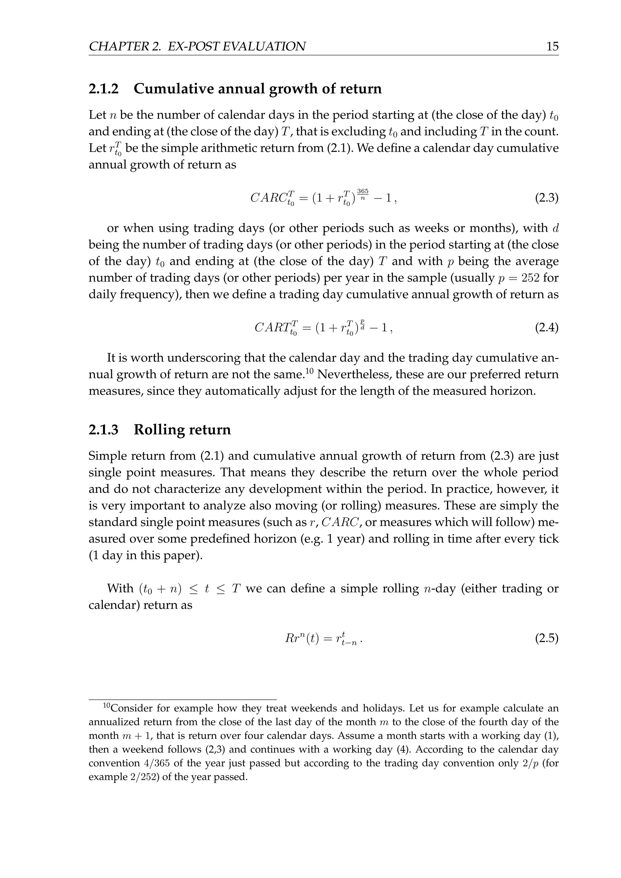
22. CHAPTER 2. EX-POST EVALUATION 17
Fig. 2.7: Empirical distribution (histogram) of the monthly returns of the index S&P 500
with net (after tax) reinvested dividends. The −10% bin represents returns from the inter-
val (−∞, −0.1] and for example the 2% bin represents returns from the interval (0.01, 0.02].
Similarly for other bins. Data source: Bloomberg
The figure (2.7) displays the empirical distribution (histogram) of the monthly re-
turns of the net total return American equity index S&P 500.
2.2 Risk measures
Investors tend to focus most of their time and effort on generating returns. However,
it is very often the case that their wrong expectations about risk will not only erase
returns that an investment has generated, but also force them to abandon their in-
vestments too soon and with a loss. The thorough understanding and analysis of the
concept of risk is therefore crucial. We devote this section to the most widely used
analytically quantifiable measures of risk. The risk criteria difficult to measure will be
described in section (2.6).
Beginning with this section, we will also describe advantages and disadvantages
of the measures discussed, providing empirical charts where appropriate.

23. CHAPTER 2. EX-POST EVALUATION 18
2.2.1 Volatility
The most widely used measure of the risk is without any doubt volatility. Historical
volatility (or standard deviation)11
can be verbally described as variation of returns of
an investment around their mean return. More precisely, sample historical volatility is
defined as follows:
σf
=
1
n − 1
n∑
i=1
(ri − ¯r)2 , (2.6)
where n is the length of the return sample12
, ri denotes return rt0+i
t0+i−1 from (2.1), f
denotes the frequency at which we calculate the volatility and ¯r = 1
n
∑n
i=1 ri.
Following calculation may be performed at any desired frequency, that is, i may
refer to day, week or month. One then obtains daily, weekly or monthly volatility. For
the purposes of comparing volatility with return or other measures, it is important to
standardize all of the measures used at a given (same) frequency. We prefer (and will
use throughout the paper) an annualization13
. We have already mentioned that we will
use the daily frequency as a tick, that is the smallest time unit. Hence, when f denotes
the daily frequency, i represents days and our annualized volatility is calculated as
follows:
σ =
√
p · σf
, (2.7)
where p stands for the number of trading days (or other periods corresponding to
the frequency f) per year. We emphasize once again that we are using the number of
trading days and not the number of calendar days per year.
We may (and will later in the practical section) calculate also the (n−trading day)
rolling annualized historical volatility:
11
Modeling of the volatility is a very comprehensive topic. We may refer a reader interested in more
details for example to [10]. The more complex methods of calculating volatility such as EWMA (expo-
nentially weighted moving average model) or GARCH (generalized autoregressive conditional hete-
roskedastic model) are very useful for the forecasting or modeling purposes. For the purposes of evalu-
ation of the historical performance, however, historical volatility as one of the means of risk comparison
among investments should be sufficient. We will therefore utilize historical volatility throughout the
paper.
12
Note that here we are using trading days, not calendar days, because the returns are realized only
on the trading days.
13
In practice, we often observe incorrect comparisons of return against volatility (even on websites
devoted to investment modeling), when return is annualized and volatility is not. Sometimes even two
volatilities calculated at different frequencies are being compared to each other.

24. CHAPTER 2. EX-POST EVALUATION 19
Rvn
(k) =
p
n − 1
k−1∑
i=k−n
(
ri − ¯rn(k)
)2
, (2.8)
where k is the trading day of calculation, p number of trading days per year, d is
the number of trading days in the sample, (n + 1) ≤ k ≤ d and ¯rn(k) = 1
n
∑k−1
i=k−n (ri).
Although volatility is the most widely adopted risk measure for an investment, it
has its flaws and does not describe some of the major risks of an investment. Consider
the following real life example why volatility may not be sufficient to assess the risk
of an investment.
An investor afraid of a potential financial crisis decided to make an investment on
1.1.2008 into the American high yield bonds. He calculated daily historical volatility
of the American high yield bond index from the last 5 years, which he annualized and
correctly arrived at a final figure of 3.58% p.a.. To be sure whether his decision was
good, he also calculated the same volatility but from American treasury bonds (with
the maturity of 7 to 10 years), which are considered as „safe heaven” investments. He
again correctly arrived at value 5.49% p.a.. He compared the volatility of his high yield
investment idea with that of the safe treasuries and because the volatility of high yield
bonds was even lower than the volatility of treasuries, he made his investment.
Fig. 2.8: iBoxx USD Liquid High Yield Index from 1.1.2003 to 31.12.2008 and illustration of its
maximum drawdown. Data source: Bloomberg
However, exactly a year later this investor more than just regretted his investment.
He observed the decline of the investment from its peak to its through of more than

25. CHAPTER 2. EX-POST EVALUATION 20
30%. See the figure (2.8). What has the investor done wrong? The list of the mistakes
could be quite comprehensive, hence we name just a few. For example, he did not ana-
lyze what stands behind his investment (character of the investment), he did not look
far enough into history and he did not calculate a very important measure, maximum
drawdown (see section (2.2.2)).
Semi-deviation
One of the disadvantages of the standard deviation is that it penalizes also the high
deviation above the mean, that is, extremely positive returns. This may influence the
results substantially when the distribution of returns is asymmetric and does not re-
semble the normal distribution, which is often the case in an investment reality. The
desired property of semi-deviation is that it considers volatility only of the below-
mean returns (annotation same as in (2.6)):
σf
S =
1
n − 1
n∑
i=1
ri<¯r
(ri − ¯r)2 . (2.9)
Downside deviation
Although semi-deviation does not penalize returns above the mean as opposed to
standard historical volatility, it may still penalize positive returns (when the mean re-
turn is high), or not penalize negative returns (when the mean return is low). The
property of penalizing only negative returns (or only the returns below a specific th-
reshold) is the essence of another measure, downside deviation. We use the same an-
notation as in (2.6) and denote as MAR a pre-specified minimum acceptable return
threshold:
σf
D =
1
n − 1
n∑
i=1
ri<MAR
(ri − MAR)2 . (2.10)
Practical usefulness of the downside deviation can be demonstrated with the fol-
lowing example. In the period starting on 11.12.2013 and ending on 11.12.2014 the
Russian ruble depreciated strongly against euro, see the figure (2.9). An investment
in euro against ruble was therefore a very profitable investment. Now, let us consider
the volatility of this EUR/RUB currency pair. Annualized daily historical volatility for
the period measured stands at 16.63% p.a.. However, annualized daily downside de-
viation (with MAR = 0) is only 9.99% p.a.. This difference is caused by the fact, that
majority of the volatility of the currency pair was caused by positive performance.
This is already adjusted for by the downside deviation, hence its value is lower.

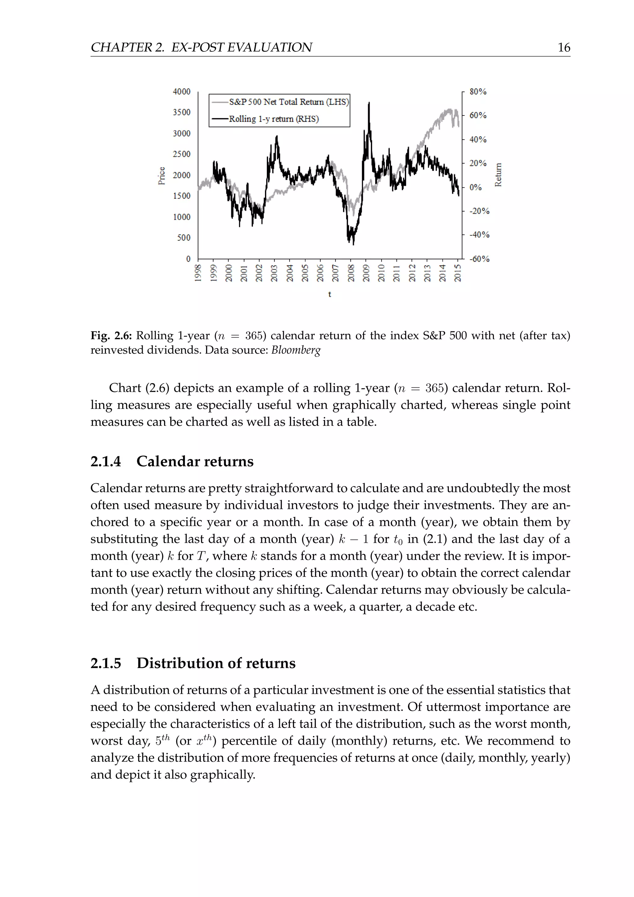
26. CHAPTER 2. EX-POST EVALUATION 21
Fig. 2.9: Currency pair euro against Russian ruble (spot rate). Data source: Bloomberg
2.2.2 Maximum drawdown
One of the most important risk measures (if not the most important one) is the maxi-
mum drawdown. Simply said, it is the worst case historical loss of an asset. The worst
case loss means a loss from the top to the bottom. In other words it is the loss realized
by an investor who bought an investment at the worst possible time and sold again at
the worst possible time.
If Pt is a price of an asset at time t (either trading or calendar day), then we can
define the maximum price of an asset up to the time t as
Mt = max
u∈[t0,t]
Pu , (2.11)
the drawdown at time t as
DDt =
Pt
Mt
− 1 , (2.12)
(which creates an entire time series of the drawdown {DDt}T
t=t0
) and consequently
the maximum drawdown during the entire window under inspection, up to the time
n as
MDDn = min
t∈[t0,n]
DDt . (2.13)
Why should the drawdown be so important in a risk management? The volatility
gives us a clue about the distribution of returns or about the probability of the move

27. CHAPTER 2. EX-POST EVALUATION 22
of an investment in an either direction. However, it does not describe at all how much
exactly an actual investor could have lost on his investment in the history. And preci-
sely this is described by the maximum drawdown.
We may (and will later in practical section) calculate also the empirical distribution
of the drawdowns. The distribution of the drawdowns may be calculated in two dif-
ferent ways. Firstly, it may be calculated from the entire time series sample (TS) of the
drawdown as:
QTS
(α) = {x : P(DDT
t0
≤ x) = α} , (2.14)
where Q is the empirical quantile function and t0, T denote the beginning and the
end of the evaluation period respectively. Percentile calculated from the entire time
series sample of the drawdown may, at least optically, understate (or even overstate)
the drawdown figure. Consider for example (of an understatement) the median of the
time series of the drawdown for a fictive asset from the figure (2.10). This asset spends
most of the time near 0% drawdown but once in a few weeks generates a loss.
Fig. 2.10: The time series of a price of a fictive asset and the time series of the drawdown of an
asset.
The median of the time series of the drawdown for this asset is 0% (because majo-
rity of the time the drawdown of an asset is 0). The problem is that we know that the
asset experiences the drawdown quite regularly and hence the median calculated in
the way above is misleading.
The second way how to calculate the distribution of the drawdowns is to create a
list of all of the local maximum drawdowns that an asset has experienced in the period

28. CHAPTER 2. EX-POST EVALUATION 23
under investigation. A new local drawdown begins whenever Pt < Mt and subsequ-
ently ends when Pt = Mt. We may calculate the list of local maximum drawdowns as
follows.
Firstly, take an entire time series of the drawdown {DDt}T
t=t0
and append 0 as a
last (T + 1) value. Secondly, divide this sample in such non-overlapping, non-empty
subsamples starting on some (ta +1) and ending on some (tb −1) that DDta = DDtb
= 0
and DDtc < 0 for all ta < tc < tb, while naturally ta >= t0 and tb <= (T + 1). All of the
non-zero values of {DDt} are now a part of some subsample, which we may denote
by Si. If we now for each Si take a minimum over all {DDt} which are part of Si, we
create a list of all of the local maximum drawdowns. That is,
LMDDi = min
t
DDt∈Si
DDt , ∀i . (2.15)
To make this obscure definition of a practically very simple calculation more clear,
we provide an example. Consider a following
{DDt}10
1 = {0%, −0.5%, 0%, 0%, −1%, −2%, −0.5%, −1%, 0%, −0.7%} .
The resulting list of local maximum drawdowns is {−0.5%, −2%, −0.7%}. We obtained
it by taking the minimum of each of the subsamples
S1 = {−0.5%}, S2 = {−1%, −2%, − 0.5%, −1%}, S3 = {−0.7%} .
Henceforth, we will be using the terms list of local maximum drawdowns and list of dra-
wdowns interchangeably.
Lets denote the list of local maximum drawdowns {LMDD1, LMDD2, . . . , LMDDn}
created in such a way during the period beginning with t0 and ending with T as
DDLT
t0
. Now we may calculate the empirical distribution (and quantile) from this list
as:
QL
(α) = {x : P(DDLT
t0
≤ x) = α} . (2.16)
To give a specific example, the list of local maximum drawdowns for a fictive asset
from the figure (2.10) is {−2%, −6%, −4%} and hence the median drawdown from the
list is QL
(0.5) = −4%.
We will now discuss one of the shortcomings of the maximum drawdown figure
and how we may overcome it.
The figure (2.11) illustrates why the maximum drawdown solely is not sufficient
for assessing the risk of an investment. Consider the two indices in the chart. Their
maximum drawdown is almost the same (−54.5% for MSCI Europe and −55.71% for
S&P 500). But the main difference is how long did the drawdown last. The time length
of the drawdown of MSCI Europe was much longer than that of S&P 500, which reco-

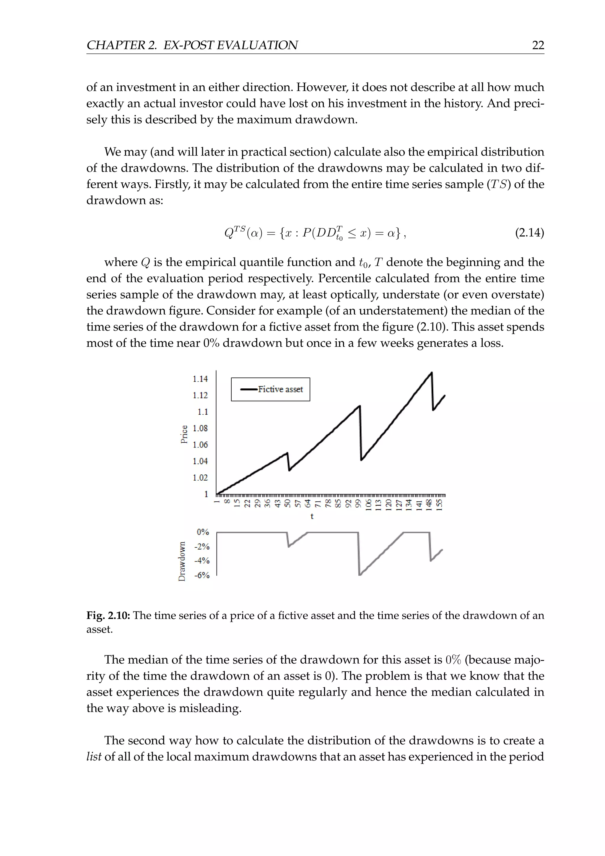
29. CHAPTER 2. EX-POST EVALUATION 24
Fig. 2.11: MSCI Europe Local Net Total Return index and S&P 500 Net Total Return index from
30.12.2005 to 31.12.2013, normalized to the value of 1 as of 30.12.2005. Data source: Bloomberg
vered back to its price maximum approximately 9 months earlier. This characteristic
of the drawdown is described by the next measure.
2.2.3 Time to recovery
Time to recovery is the time (in calendar days) measuring how long did an investment
take to recover from its drawdown back to the new maximum. In other words, it is
the time length of the drawdown. It can be measured for every drawdown and the
distribution may be calculated of them. The most widely used form is the longest
(maximum) time to recovery over the whole time sample under inspection. If we use
the same annotation as in (2.11), we define the time to recovery at time t as
TTRt = t − arg max
u∈[t0,t]
Pu , (2.17)
and the maximum time to recovery as
MTTRn = max
t∈[t0,n]
TTRt . (2.18)

30. CHAPTER 2. EX-POST EVALUATION 25
2.2.4 Value at risk14
Value at risk is the estimated maximal loss on an asset (or portfolio) on a given time
horizon with a given level of confidence. If we denote by α the confidence level, by L
the unknown loss of a portfolio and by l the actual specific value of the loss, which we
aim to solve for, then the general definition of value at risk is as follows:
V aRα = inf(l ∈ R : P[L > l] ≤ 1 − α) (2.19)
Many methods of calculating value at risk do exist in practice. The simplest is the
non-parametric historical simulation which is a (1 − α) − %th quantile of historical asset
(or portfolio) returns on a given time frame. Parametric methods make specific as-
sumptions about the distribution of the returns (normal, student or many other) and
then calculate value at risk as expected mean return minus multiple of standard de-
viation (corresponding to a specific distribution). Other methods model asset returns
via GARCH (or another) model and calculate value at risk among this framework. All
of the aforementioned deal with the expected loss within a certain level of confidence.
On the other hand, conditional value at risk analyzes the loss once it happens, that is,
models the tail risk. We will not go into more detail and instead refer a reader to [14].
For the purposes of this paper we will define value at risk based on a parametric
method assuming normal distribution and calculate it as follows:
V aRα = ¯r + zα · σ , (2.20)
where ¯r is a mean return (calculated from the single tick frequency - daily in this
paper) in a period under investigation, zα is the α-quantile of the standardized normal
distribution and σ is the volatility (not annualized) of single tick returns from (2.6).
The main disadvantage of value at risk is that (with an exception of the historical
simulation) it is model dependant. More advanced models need to be calibrated and
often contain many parameters which can introduce over-fitting. Moreover, value at
risk typically utilizes only some recent data history and does not take into account
whole history of an asset. The outcome is just a single number which may and may
not be helpful in a specific cases. Value at risk is therefore a perfect tool for banks to
model their capital requirements, but less practical tool for investment analysts.
14
There are entire books focused on the topic. We do not aim to cover all existing variations and the
details of the calculation, but we recognize the value and importance of this statistic, thus we do list it
here in a simple form.

31. CHAPTER 2. EX-POST EVALUATION 26
2.3 Return to risk measures
One of the most challenging and crucial roles of an investment analyst or a portfolio
manager is an assessment of a particular investment’s return against its risk. There are
many types of investors. One group focuses on finding the assets with the best return
to risk profile. Another group does have specific return objective and aims to find in-
vestments capable of providing such a return, with the lowest risk possible. Also vice
versa, many investors have a given risk target which should not be exceeded and try
to maximize their return subject to this risk hurdle. All of the above mentioned need to
very thoroughly analyze and use return to risk measures. In general, the higher return
to risk, the better. However, special caution has to be applied in case of the negative
return to risk values, because many of the common measures have an inverted (or
highly altered) logic in such a case.15
2.3.1 Sharpe ratio
Likely the most famous return to risk measure is that of William F. Sharpe introduced
in 1966 in [1]. The Sharpe ratio is simply the excess return of an asset (return minus risk
free return) divided by asset’s volatility. An ex-ante (forward looking) Sharpe ratio is
defined as follows:
SHRe =
E[r − rf ]
σ
, (2.21)
where r is a single tick (daily in this paper) return from section (2.1), rf a single tick
risk free rate and σ volatility from (2.6), calculated from single tick returns. The choice
of a risk free rate is a topic on its own. In practice the return of short term (3 months
or shorter) treasury bills is often used. However now, in 2016, having witnessed short
term bills of numerous countries crossing zero and being in a negative territory, the 0
value is increasingly being used as rf .
Since this chapter deals with an ex-post evaluation we will define the Sharpe ratio
as
SHR =
CARTT
t0
− rf
σT
t0
, (2.22)
15
We will not be adjusting each measure (and thus providing a special framework) for the case of
negative values. Negative return to risk measures are caused almost always by the negative numerator,
that is negative excess (or classic) return of an investment. In that case special logic applies. Take an
example of the Sharpe ratio from section (2.3.1). It compares excess return against volatility. When it
is positive, the higher Sharpe ratio means better risk adjusted performance (higher returns with lower
volatility). When it is negative, the question what is now better arises. A higher Sharpe ratio, that is
less negative return with high volatility or a lower Sharpe ratio, that is more negative return with lower
volatility? The answer is not straightforward and we will not focus on answering it.

32. CHAPTER 2. EX-POST EVALUATION 27
where CARTT
t0
is not the expected return but annualized historical return from
(2.4). σT
t0
is the annualized historical volatility (here we denote by subscript t0 and su-
perscript T the start and end of the horizon from which the volatility is calculated)
from (2.7) and rf is the annualized risk free rate corresponding to the period under
investigation. Everything is calculated utilizing trading days.
We may calculate also the (n−trading day) rolling annualized Sharpe ratio:
RSHRn
(t) =
CARTt
t−n − rf (t)
Rvn(t)
, (2.23)
where CARTt
t−n is the trading day cumulative annual growth of return from (2.4),
rf (t) is the annualized risk free rate corresponding to the period [t − n, t] (for example
the average of the risk free rate during that period) and Rvn
(t) is the rolling annualized
historical volatility from (2.8).
Fig. 2.12: Rolling 1-year (252-trading day) annualized Sharpe ratio of the S&P 500 net total
return index. Data source: Bloomberg
The figure (2.12) depicts the rolling 1-year (252-trading day) annualized Sharpe
ratio of the S&P 500 net total return index.
The main disadvantage of the Sharpe ratio lies in its reliance only on volatility
as a risk measure. Consider again the example from section (2.2.1) and figure (2.8).
Now an investor also calculates the 5 year annualized Sharpe ratio of high yield bonds
and gets a value of 3.42 which is almost triple when compared to 1.21 of treasury
bonds. This may again lead to a wrong conclusion (as already shown in the section
mentioned above) that high yield bonds are undoubtedly the better investment. It is
important that an investor considers also many other aspects such as drawdown, time
to recovery, character of an investment, credit risk and many other, rather than solely

33. CHAPTER 2. EX-POST EVALUATION 28
the Sharpe ratio.
2.3.2 Sortino ratio
The Sortino ratio (introduced by Sortino and van der Meer in [5]) is very similar in
nature to the Sharpe ratio. The difference between the two is the usage of a predefined
hurdle rate, minimum acceptable return (MAR), instead of a risk free rate. This hurdle
rate is also incorporated into the altered standard deviation calculation, so that only
returns below the hurdle rate are used in the calculation.
SRR =
¯rT
t0
− MAR
σD
, (2.24)
where ¯rT
t0
is the average (single period, that is daily, not annualized) return from t0
to T, MAR is the aforementioned minimum acceptable return threshold (of the same
frequency) and σD is the (single period, that is daily, not annualized) downside de-
viation from (2.10). Throughout the paper we will use the annualized Sortino ratio (to
stay in line with all other measures), which we obtain as follows:
SRRa
=
CARTT
t0
− MARa
√
p · σD
, (2.25)
where CARTT
t0
is from (2.4), p is the number of trading days per year, MARa is the
annualized minimum acceptable return and σD is the (single period, that is daily, not
annualized) downside deviation from (2.10). The main advantages and disadvantages
of using the ratio correspond with that for the Sharpe ratio, with the difference of a
better penalization of only below-hurdle returns for the Sortino ratio.
One of the important deficiencies of the Sharpe ratio and the Sortino ratio is that
they do not (fully) take into consideration if the (positive) performance of an inves-
tment was achieved consistently throughout the whole period under investigation
or just during a short time period. Consider the following example of the two equ-
ity market indices - Chinese Shanghai Composite and American small capitalization
Russell 2000. During the period depicted in the figure (2.13) both appreciated roughly
the same in their value achieving almost identical cumulative annual growth of re-
turn. If we choose the same MAR equal to 0 for both of them, then the only material
difference between the two indices (relevant for the calculation of the Sortino ratio)
is their different downside deviation. Volatility of Shanghai Composite was slightly
higher than for the Russell 2000 in the period under investigation, which resulted into
the Sortino ratios of 1.61 and 1.93 respectively. Now although the Sortino ratio for
the Russell 2000 is 20% higher than for the Shanghai Composite, the ratio ignores the
path through which these indices achieved their terminal value. By visual inspection,
the path of the Russell 2000 was much more linear (and hence more stable) than the
path of the Shanghai Composite. This is much better reflected in the value of another

34. CHAPTER 2. EX-POST EVALUATION 29
Fig. 2.13: Shanghai Composite price index and Russell 2000 price index from 11.6.2012 to
3.4.2015, normalized to the value of 1 as of 11.6.2012. Data source: Bloomberg
measure - the DVR ratio.
2.3.3 DVR ratio
The DVR ratio (named most likely after its author David Varadi - we may refer a
reader to his blog [15]) connects the Sharpe ratio with R2
from the linear regression of
the price of an investment against time:
DV R = SHR · R2
, (2.26)
where SHR is the Sharpe ratio from (2.22) and R2
is the coefficient of determination
from the following linear regression (Pt being the price of an asset at the discrete time
tick t and d number of trading days):
Pt = α + β · t , t = 1, . . . , d . (2.27)
Now consider the recent example from the section (2.3.2). The R2
for the regression
of the Shanghai Composite index against time is 0.32 and for the Russell index 0.88.
That results into values of DV R of 0.34 and 1.16 respectively. The difference of 239%
between the DV R ratios is now much higher than the difference between the Sortino
ratios16
and better reflects the difference in their price paths.
16
The difference in DVR ratios is also much higher than the difference between the Sharpe ratios
which stands at 22% for the Sharpe ratios of 1.09 and 1.33 for the Shanghai Composite and the Russell
2000 respectively.

35. CHAPTER 2. EX-POST EVALUATION 30
2.3.4 Calmar ratio
The Calmar ratio simply compares the return of an investment against its maximum
drawdown:
CR =
CARTT
t0
MDD
, (2.28)
where CARTT
t0
is from (2.4) and MDD (from the same corresponding period) is
from (2.13).
Fig. 2.14: S&P 500 Net Total Return index and MSCI Emerging Markets Net Total Return USD
index from 13.11.2008 to 24.10.2013, normalized to the value of 1 as of 13.11.2008. Data source:
Bloomberg
Now consider an example in the figure (2.14) as an illustration why the Calmar ra-
tio (and the maximum drawdown as well) is very sensitive to the specific period du-
ring which we measure it and hence it may not be sufficient to use it alone as a measure
to compare investments. During the period under investigation the S&P 500 returned
15.91% p.a. while suffering the maximum drawdown of −27.31% and the MSCI Emer-
ging Markets returned 17.48% p.a. with the maximum drawdown of −30.06%. Their
Calmar ratios are almost identical (0.58 both), yet, when examining the chart above,
an investor would be tempted to prefer S&P 500 because of its smoother price path.

36. CHAPTER 2. EX-POST EVALUATION 31
One of the ways how we can mathematically describe smoothness for an investment
is by looking at the frequency, or percentile of drawdowns.
The main disadvantage of using the Calmar ratio is that it does not take into ac-
count a frequency and length of drawdowns (because MDD represents just a sin-
gle number from the entire sample). This can be hardly achieved by examining just
one number (and not the whole historical evolution of the drawdowns), but can be
partially accomplished if we replace the maximum drawdown in the denominator of
(2.28) by some percentile (greater than 0) of the drawdown.
2.3.5 CAR to Xth percentile of drawdown
Useful modification of the Calmar ratio is achieved by replacing the maximum dra-
wdown in the denominator of (2.28) by a percentile (quantile) of the drawdown. Le-
vels such as 1%, 5%, or 50% are often used in practice. This way we are able to lessen
the sensitivity of the Calmar ratio (calculated from the event (or single point) sensitive
maximum drawdown number) by using information from the distribution of drawdo-
wns. We may calculate the ratio in two different ways, differing in whether we use the
quantile of the entire time series of the drawdown (TS) in the denominator of the ratio
or the quantile of the list (L) of the drawdowns (see also section (2.2.2)).
CPDTS
(x) =
CARTT
t0
QTS(x)
, (2.29)
CPDL
(x) =
CARTT
t0
QL(x)
, (2.30)
where CARTT
t0
is the trading day cumulative annual growth of return from period
t0 to period T from (2.4) and QTS
(x) and QL
(x) are the x-th quantiles of the time series
of the drawdown and of the list of local maximum drawdowns from (2.14) and (2.16)
respectively.
If we now calculate CPDTS
(5%) for the recent example from the section (2.3.4), ins-
tead of very close values of the Calmar ratio (0.58 for both investments) we now get
much more distinct values of 1.19 for S&P 500 and 0.8 for MSCI Emerging Markets.
This clearly favors American equities because of their less frequent losses (drawdo-
wns).
2.3.6 Omega ratio
The main shortcoming of the measures described in the paper so far is that they do
not fully take into account an entire distribution of returns (the exact shape of the
distribution). For example two assets may have identical Sharpe ratios, but their return

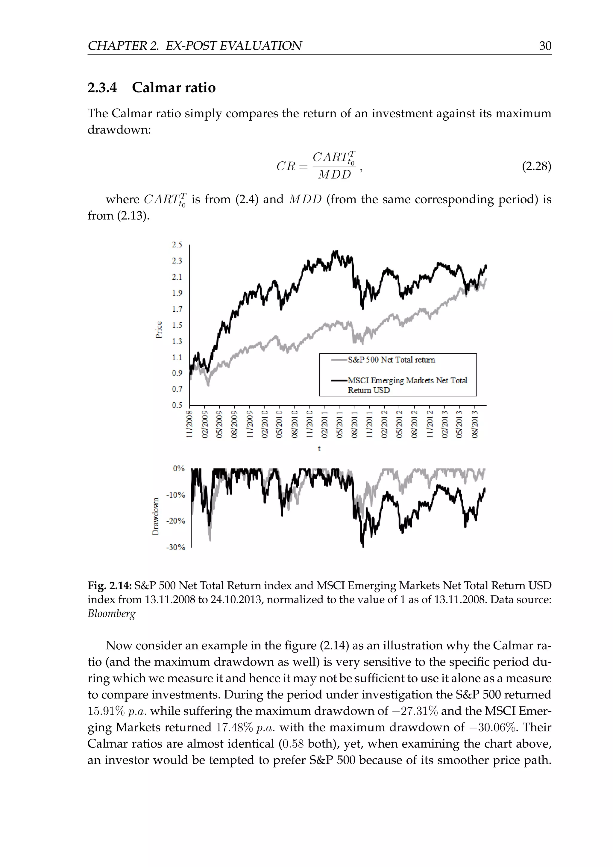
37. CHAPTER 2. EX-POST EVALUATION 32
distributions may be entirely different. The Omega ratio introduced in [6] incorporates
also the higher moments than just the first two - mean and variance of the portfolio
returns distribution. The Omega ratio uses a threshold (minimum acceptable return) and
calculates the ratio of the upside above the threshold against the downside below the
threshold. The calculation is as follows:
Ω(MAR) =
∫ b
MAR
(1 − F(x))dx
∫ MAR
a
F(x)dx
, (2.31)
where F(x) is the empirical cumulative distribution function of returns of an asset,
MAR is the minimum acceptable return threshold, a is the minimum return and b is
the maximum return. An illustration of how the Omega ratio is calculated is depicted
in the figure (2.15). More on the analysis of the Omega ratio can be found for example
in [16] or [17].
Fig. 2.15: Empirical cumulative distribution function of the daily returns of S&P 500 Net Total
Return index from 31.12.2014 to 31.12.2015, the minimum acceptable return threshold chosen
as 0% and an illustration of the Omega ratio (ratio of the surface of the region marked by „U”
against the surface of the region „D”). Data source: Bloomberg
2.3.7 Return to maximal loss
This measure compares the average return of an asset (on a given time horizon and
on a given frequency) against the worst return. It is useful to calculate it on different

38. CHAPTER 2. EX-POST EVALUATION 33
frequencies, that is, as a daily return (d), weekly return (w), monthly return (m) or
yearly return (y):
RMLf
= −
¯r
mini∈[t0,T] (ri)
, (2.32)
where f denotes the desired frequency (d, w, m, y) of the returns r.
2.3.8 Ulcer performance index
The Ulcer performance index belongs to the group of measures which compare a re-
turn of an investment against its risk. It is different from the other similar measures
because it uses a unique measure of risk - the sum of squares of the time series of
the drawdown of an asset (the Ulcer index). This is distinct from the Calmar ratio or
from the CPD because the two aforementioned use just a single point (maximum dra-
wdown or percentile of the drawdown) in the calculation. On the contrary, the Ulcer
performance index incorporates the entire drawdown evolution into the calculation.
It was introduced by P. Martin in [18].
UPI =
CARTT
t0
− rf
UI
, (2.33)
where CARTT
t0
is the trading day cumulative annual growth of return from period
t0 to period T from (2.4), rf is the annualized risk free interest rate and UI is the above
mentioned Ulcer index defined as:
UI =
√
∑d
t=1 (DDt)2
d
, (2.34)
where DDt is the time series of the drawdown from (2.12) and d is the number of
trading days in the period under inspection.
2.4 Other quantifiable measures
Some of the measures may be hardly classified into one of the above mentioned secti-
ons. They are neither just the return or risk measures, nor measures comparing return
against the risk. Such measures include higher moments of an investment returns and
also some more complex ratios. All of these are however still important for the evalu-
ation of investment strategies.
2.4.1 Statistical significance
The majority of research papers involved in an analysis of potential investment stra-
tegies test these strategies for statistical significance. In case of research papers which

39. CHAPTER 2. EX-POST EVALUATION 34
deal with an evaluation of existing investments (or funds), tests for a statistical signi-
ficance are used less often. Investors in such funds are much more interested in the
already realized return and risk characteristics of an investment rather than in their
statistical significance.
Suppose that returns of an investment ri =
Pti
Pti−1
− 1 , i = 1, . . . , n (where n is the
number of return observations in the sample and hence tn = T) are independent,
identically distributed and follow the normal distribution N ∼ (µ, σ2
), then
¯X − µ
S
√
n ∼ tn−1 , (2.35)
where ¯X = 1
n
∑n
i=1 ri , S =
√
1
n−1
∑n
i=1 (ri − ¯X)2 , µ is the unknown true mean
return of the whole population and tn−1 is the Student’s t-distribution with (n − 1)
degrees of freedom. One may then formulate a hypothesis of the form
H0 : µ ≤ MAR vs. H1 : µ > MAR ,
where MAR is our minimum acceptable return (often set to 0, which is the special
case). The test statistic for such hypothesis based on (2.35) is
TS =
¯X − MAR
S
√
n . (2.36)
We reject the null hypothesis H0 if TS > tn−1,α , where α is our pre-specified
level of significance and tn−1,α is the α-percent critical value ((1 − α) percent quantile)
of the t-distribution with n − 1 degrees of freedom. The interesting property of the test
statistic is that if MAR = rf , where rf is the risk free rate used in the calculation of
the daily Sharpe ratio17
, then TS =
√
n · SHR and we are actually testing if the scaled
Sharpe ratio exceeds the critical value of the t-distribution. See more for example in
[19].
Although many of the above mentioned assumptions do not hold in reality (returns
are definitely not independent and also the rejection of H0 does not imply that H1
is true), many practitioners use the test to assess if the mean return of the fund (or
strategy) is statistically greater than 0 (or another MAR threshold)18
.
17
In (2.22) we calculated the Sharpe ratio from annualized return and annualized standard devia-
tion. The Sharpe ratio may be also calculated from daily returns (not annualized) and daily standard
deviation (not annualized). We denote this as the daily Sharpe ratio.
18
In practice we often witness the race for the highest t-statistic when creating investment strategies,
which is quite tricky, because statistically, higher t-statistic does not imply better strategy. The only
implication which we can make is the rejection of the null hypothesis.

40. CHAPTER 2. EX-POST EVALUATION 35
Factor models
More often than just testing for a significance of the return being greater than zero,
practitioners do run a series of regressions of the form
ri = α + β1 · X1 + β2 · X2 + . . . + βk · Xk + ϵi , i = 1, . . . , n , (2.37)
where ϵi is the error term and Xi are some common known factors such as the pas-
sive market return or famous Fama and French factors ([7]) value and size or many
other. Then the main analysis involves testing of the statistical significance of the α
coefficient, or in other words, if the excess return of a fund (or strategy) cannot be ex-
plained by just the common already existing market factors. For the very nice review
of existing factor models see for example [8].
The problem with p-values is that their statistical significance does not imply eco-
nomical significance. That is the reason why practitioners very scarcely base their in-
vestment decisions on the p-values. Hence, p-values do often serve as a necessary
but not sufficient condition for accepting a potential strategy. The strategy validation
through statistical significance is however much more often used for an ex-ante eva-
luation of strategies, rather than for an assessment of already existing live strategies
(ex-post). We will not focus on evaluating strategies by means of a statistical signi-
ficance in this paper, because of the already mentioned reasons regarding uncertain
economical significance.
2.4.2 Skewness
Useful measure from the standard statistical analysis which helps to assess the tail
risk (or reward) of an investment is skewness. Roughly speaking, positive skewness
implies heavier right tail of the distribution (that is an investment more prone to the
extreme positive returns) and negative skewness vice versa, the heavier left tail of
the distribution (that is an investment more prone to the extreme negative returns).
Skewness of a symmetric distribution equals zero. The calculation for the sample ske-
wness goes as follows:
SK =
1
n
∑n
i=1 (ri − ¯r)3
( 1
n−1
∑n
i=1 (ri − ¯r)2
)3/2
, (2.38)
where ri are the simple one tick asset returns, n is the number of return observati-
ons in the sample and ¯r = 1
n
∑n
i=1 ri.
Skewness is just a single value which has its advantages and disadvantages as well.
The main advantage is an easy comparison across different assets. The disadvantage
is that it does not tell us anything about the structure of the tails of the asset returns’

41. CHAPTER 2. EX-POST EVALUATION 36
distribution. One asset may have much higher skewness than the other asset and still
the left tail risk (measured by other measures such as e.g. maximum drawdown) of
the first asset may be higher than that of the second asset.
Consider an example of the 10 year sample of monthly returns of the two indi-
ces, American equity market index S&P 500 and American iBoxx high yield bond
index from the figure (2.16). Skewness of the S&P 500 monthly returns is −0.76 and
skewness of the iBoxx high yield bond monthly returns is −1.28. Both of them are
negative, which suggests higher probability of extreme negative, rather than positive
returns. Skewness of the high yield bond index is almost 70% lower than skewness
of the equity market index. One may conclude that the left tail risk of the high yield
bonds should be higher than that of equities. However, when we look at the maximum
drawdown (see (2.13)) of both indices, we get the value of −55.7% for the S&P 500 and
−32.9% for the iBoxx high yield. In reality, the left tail risk (when using maximum dra-
wdown as a measure) was actually almost 70% higher (and not lower) for the equity
market index when compared to the high yield bond index.
Fig. 2.16: Monthly returns of the S&P 500 Net Total Return index and iBoxx USD Liquid High
Yield Index from 1.1.2006 to 31.12.2015. The −10% bin represents returns from the interval
(−∞, −0.1] and for example the 2% bin represents returns from the interval (0.01, 0.02]. Simi-
larly for other bins. Data source: Bloomberg
2.4.3 Kurtosis
Kurtosis is the second measure from the standard statistical analysis which helps to
describe the tail risk of an asset. Again roughly speaking, kurtosis measures how he-
avy are the tails of the distribution of an asset returns (or in other words the „peaked-
ness” of an asset returns). The higher the kurtosis the heavier the tails of the distribu-

42. CHAPTER 2. EX-POST EVALUATION 37
tion. Kurtosis of a standard normal distribution equals 3. Higher (lower) kurtosis of
returns than 3 thus implies that an asset is more (less) prone to extreme movements
of an unknown direction (either positive or negative). The calculation of the sample
kurtosis is as follows:
KU =
1
n
∑n
i=1 (ri − ¯r)4
( 1
n−1
∑n
i=1 (ri − ¯r)2
)2 , (2.39)
where ri are the simple one tick asset returns, n is the number of return observati-
ons in the sample and ¯r = 1
n
∑n
i=1 ri.
Again, kurtosis does tell us how heavy the tails of the distribution of returns are
(when compared to other distributions), but does not tell us other information about
the structure of the tails. When we again analyze the example from the section (2.4.2)
and from the figure (2.16) and calculate the sample kurtosis for both indices, we get
the value of 1.78 for the S&P 500 equity index and 8.85 for the iBoxx high yield bond
index. Because skewness is more negative for high yield bonds and kurtosis is again
higher for high yield bonds we now may be tempted to conclude that high yield bonds
are more prone to extreme movements than equity markets and that a probability of
an extreme negative movement is higher than that of an extreme positive movement
for high yield bonds. However, we already know that the maximum drawdown of the
equity market index was much higher than that of the high yield bonds. A lesson to
learn from this analysis is that it is crucial to take into consideration all of the informa-
tion we have about the distribution and about the asset, not just the single (or a small
subset) measure.
2.4.4 Fractal efficiency
Many investors do care a lot about smoothness and stableness of their investments
rather than about specific return or risk targets. The reasons behind preferring smo-
oth path of investments are numerous but almost all of them have one in common
- greater confidence in such an investment and thus lower probability of inapprop-
riate transactions (such as buying high and selling low) performed by investors. The
smoothness or stableness can be described by many of the already mentioned risk me-
asures and risk to return measures, but there are also measures especially developed
for measuring smoothness. First of them is the fractal efficiency.
The fractal efficiency is very simple to calculate and, roughly said, measures the
length of the price path of an investment which is compared against a hypothetical in-
vestment with the same return but linear price path. Formula for the fractal efficiency
is as follows:
FE =
PT − Pt0
∑d−1
i=1 |Pti
− Pti−1
|
, (2.40)

43. CHAPTER 2. EX-POST EVALUATION 38
where Pi is the price of an asset at time i and d is the number of trading days from
t0 to T, hence td−1 = T. For longer time horizons, where the price path tends to create
a geometric (exponential) growth path, the logarithmic fractal efficiency ratio should
be used:
LFE =
ln PT − ln Pt0
∑d−1
i=1 | ln Pti
− ln Pti−1
|
. (2.41)
2.4.5 K-ratio
The K-ratio introduced by L. Kestner in [20] and [21] is another from the series of
measures which aim to quantify the linearity (or stableness) of an investment. The
K-ratio is slightly more sophisticated than the fractal efficiency and should be able to
better capture the degree of linearity of an asset. The K-ratio is essentially the scaled
t-statistic of the beta coefficient from the regression of a (logarithm of the) price of
an asset regressed against time. This cumbersome verbal description is much easier
understood in a formula:
KR =
ˆβ
SE(ˆβ)
·
√
p
d
, (2.42)
where d is the number of observations in an entire sample, p is the number of
observations per calendar year (that is frequency)19
, SE is the standard error and ˆβ is
an estimate of the beta coefficient from the following regression:
ln Pt = α + β · t + ϵt , t = 1, . . . , d . (2.43)
If it was not for the scaling factor
√
p/d then the K-ratio would be essentially just
the t-statistic of the beta coefficient. In order to compare return streams of differing
lengths and varying periodicity an aforementioned adjustment has to be made.
Now consider again an example from the section (2.3.2) and from the figure (2.13).
In the chart the price paths of the American small cap equity index Russell 2000 and
the Chinese equity index Shanghai Composite were depicted. In the period under ins-
pection, both of the indices reached a very similar terminal value (and hence almost
identical cumulative annual growth of return). The main difference is between the
path through which they arrived to that value. We have already shown in the section
(2.3.2) that volatility and downside deviation of the Shanghai Composite was higher,
which resulted into the slightly lower Sortino and Sharpe ratios for Shanghai Compo-
site. We have also shown in the section (2.3.3) that when using the DVR ratio instead
of the Sharpe or the Sortino ratio solely, the difference between the Shanghai Com-
19
If the frequency is monthly, then p = 12, if it is weekly then p = 52 and if it is daily then approxi-
mately p = 252.

44. CHAPTER 2. EX-POST EVALUATION 39
posite and the Russell 2000 widens in favor of the Russell 2000 because of its much
more linear price path. We will now calculate the fractal efficiency and the K-ratio for
both aforementioned indices to support this view. Surprisingly, the fractal efficiency
ratio for the Shanghai Composite index is higher at 0.114 than that of the Russell 2000
index at 0.096. This is the result of the fact, that the price path of the Russell 2000 was
slightly longer, although by visual inspection more linear. The K-ratio reflects this li-
nearity much better with Russell 2000 scoring a value of 1.63 against 0.41 for the Shan-
ghai Composite. The difference of 296% is even bigger than the difference between the
DVR ratios.
2.5 Benchmark related measures20
As opposed to the above used categorization, this section contains the mix of return,
risk and return to risk measures. All with regards to a specified benchmark. Bench-
mark is a predefined standard, criterion or a gauge against which a real fund or an
investment is measured and compared to. It is usually an index which is easily repli-
cable or which is similar in style to the investment under consideration. There is an
entire area of literature devoted to the right choice of a benchmark, see for example
[22], [23] or [24]. We do not aim to delve deeper into the topic of benchmarking, thus
as an example we will illustrate all of the below listed measures on a pretty straight-
forward pairs of an investment and their benchmark.
The investments under inspection will be the two most well known and most wi-
dely used American exchange traded funds investing into the emerging market equ-
ities, the iShares MSCI Emerging Markets ETF and the Vanguard FTSE Emerging Markets
ETF, both including net (after tax) reinvested dividends and including costs (that is
after fees). The benchmark used is the MSCI Daily Total Return Net Emerging Markets
index21
(index with net reinvested dividends). The risk free rate is the 3-month US LI-
BOR (London - Interbank Offered Rate, calculated by the Intercontinental Exchange).
Source for all the data is Bloomberg. The period under evaluation is 18.3.2005 - 29.1.2016
and the frequency of the time series is weekly.22
These two ETFs and the index are de-
20
The aim of this paper is primarily to provide a framework for evaluating investments on a stand-
alone basis and strategies not tied to a specific benchmark. Moreover, the choice of the benchmark is
often subjective, which introduces more bias into an evaluation. Thus, we decided to not create an
exhaustive list of all benchmark related measures and many factor models. These are used primarily
for an evaluation against benchmark factors. We instead describe just the basic and most common me-
asures, upon which the more complex ones are based.
21
The official benchmark for the iShares ETF is the aforementioned MSCI index. The official bench-
mark for the Vanguard ETF, however, is different (FTSE Emerging Markets All Cap China A Net Tax (US
RIC) Transition Index). This index unfortunately does not have a sufficiently long history. Therefore, in
our analysis we will be comparing both ETFs to the same MSCI index benchmark, which is not the
official benchmark of the Vanguard ETF. Since the purpose of this section is not to select the winning
ETF but rather to illustrate the measures, we do not consider this to be an obstacle.
22
In this section we decided to lower the frequency by one level to weekly. The reason of this change

45. CHAPTER 2. EX-POST EVALUATION 40
picted in the figure (2.17).
Fig. 2.17: iShares MSCI Emerging Markets ETF, Vanguard FTSE Emerging Markets ETF, both
including net (after tax) reinvested dividends and MSCI Daily Total Return Net Emerging
Markets index. All scaled to the base value of 1. Period presented: 11.3.2005-29.1.2016. Weekly
data. Data source: Bloomberg
2.5.1 Jensen’s alpha
The Jensen’s alpha (see [3]) is defined as the differential between the return of an asset
in excess of the risk free rate and the return explained by the market model. In other
words it is an estimate of the intercept from the regression of the excess asset returns on
the excess benchmark returns. More specifically, it is an estimate ˆα from the following
regression:
(ri − rf ) = α + β · (rb − rf ) + ϵi , i = 1, . . . , n , (2.44)
where ri is the single period return of an asset under investigation, rf is the risk
free return (of the same frequency), rb is the return of a benchmark (or in other words
market return), ϵi is the error term and n is the number of return observations in the
entire sample.
is closely related to the footnote (7). More specifically, when calculating linear regressions of returns
against some factors or when calculating a standard deviation of the differences in returns of the two
assets, noise and outliers can distort the results more heavily. It is so because we are comparing two
securities day by the day (instead of comparing only a single point measure such as the Sharpe ratio
calculated from each time series of two assets separately, as in the previous sections). The differences
between daily returns may also arise because of the different pricing hours of the markets included in
such a diverse index as MSCI Emerging Markets.

46. CHAPTER 2. EX-POST EVALUATION 41
The Jensen’s alpha of the Vanguard ETF in the period under investigation is 2.46 ·
10−3
% daily (or 0.13% p.a. annualized), with the p-value of 0.97 which is statistically
insignificant on all relevant levels of significance. Jensen’s alpha of the iShares ETF in
the period under investigation is −1.9 · 10−3
% daily (or −0.1% p.a. annualized), with
the p-value of 0.98 which is again statistically insignificant on all relevant levels of
significance. This means that both ETFs (even after fees) track the benchmark pretty
closely.
Beta
Closely related to the Jensen’s alpha is the beta coefficient. Both of them are calcula-
ted from the same capital asset pricing model from (2.44). See more on the model for
example in [9]. In contrary to the Jensen’s alpha which measures the ability of a ma-
nager or an asset to deliver additional returns when compared to the benchmark, the
beta coefficient measures the sensitivity of an investment to the market movements. It
is calculated as an estimate ˆβ of the beta coefficient from the regression (2.44). Roughly
speaking, beta equal to 1 means that should the benchmark move x% in some direc-
tion, the investment will follow with the same sensitivity of the x% in the same di-
rection. Beta greater (lower) than 1 means higher (lower) move in the same direction
than the benchmark. Negative beta means a move in the opposite direction than the
benchmark.
The beta of the Vanguard ETF is 1.02 (with the p-value of 0) and the beta of the
iShares ETF is 1.06 (with the p-value of 0). Both of the betas are statistically significant
at any level of significance. This again supports the argument that both ETFs do track
the benchmark pretty closely (even after fees).
2.5.2 Black-Treynor ratio
The Jensen’s alpha measures just the additional value of an investment (in terms of a
return only) against the benchmark and does not describe risk of this additional value
at all. To improve on this, Black and Treynor in [4] developed a simple combination of
the Jensen’s alpha and the beta coefficient to arrive at the return to risk Black-Treynor
ratio:
BTR =
ˆα
ˆβ
, (2.45)
where ˆα is the estimate of an alpha coefficient from the regression (2.44) and ˆβ is
the estimate of a beta coefficient from the same regression. In this way an investment
is penalized for being too sensitive (or even leveraged) to the movements of the bench-
mark and, on the other hand, rewarded for delivering alpha with a low degree of the
sensitivity to the benchmark.

47. CHAPTER 2. EX-POST EVALUATION 42
An annualized Black-Treynor ratio of the Vanguard ETF is 0.13% and for the iShares
ETF −0.09%.
2.5.3 Tracking error
Tracking error, similar to the correlation, measures the degree of a co-movement bet-
ween two assets but in a slightly different way. It is the standard deviation of the
difference between returns of an investment and returns of the benchmark:
TREf
=
1
n − 1
n∑
i=1
(
(ri − rb
i ) − ¯rd
)2
, (2.46)
where n is the length of the return sample, ri denotes the single period return of an
investment, rb
i return of the benchmark, f denotes the frequency at which we calculate
the volatility and ¯rd = 1
n
∑n
i=1 (ri − rb
i ). We may annualize it in the same way as in
(2.7), that is
TRE =
√
p · TREf
, (2.47)
where p stands for the number of trading weeks (or other periods corresponding
to the frequency f) per year. Our already stated original frequency is weekly, which
we annualize by p = 52.
The annualized tracking error of the Vanguard ETF is 9.7% p.a. and the annualized
tracking error of the iShares ETF is 10.6% p.a.. These tracking error values are quite
high if we take into account the fact that both of the ETFs are supposed to track the
benchmark as closely as possible. One of the explanations is technical - because of the
weekly data (which is still a quite high frequency for measuring tracking error) the
same issue with the problematic pricing of different countries as in the footnote (22)
may arise. We calculated also the annualized tracking error for the monthly data which
resulted into the values of 4.7% p.a. for the Vanguard ETF and 5.7% p.a. for the iShares
ETF. The second explanation is more fundamental. Because the emerging market com-
panies are still not developed enough, and the same applies for their stock markets, it
is much harder to track their indices than it is for their developed counterparts.
2.5.4 Information ratio
While the tracking error gives us an information about the risk that an investment
will not track the benchmark, it does not contain any information about the returns
of an investment compared to its benchmark. Both of these are incorporated into the
information ratio:

48. CHAPTER 2. EX-POST EVALUATION 43
IR =
CARTa
− CARTb
TRE
, (2.48)
where TRE is the tracking error of an investment a against its benchmark b from
(2.47) and CARTa
and CARTb
are the trading day cumulative annual growth of re-
turns from (2.4) for an investment a and its benchmark b respectively (both of them for
the entire horizon [t0, T] under investigation).
Information ratios for both of the ETFs are negative (after costs), specifically, −0.04
for the Vanguard ETF (−0.37% p.a. excess return with 9.7% p.a. tracking error) and
−0.06 for the iShares ETF (−0.66% p.a. excess return with 10.6% p.a. tracking error).
2.5.5 Treynor ratio
The Treynor ratio (see also [2]) compares return of an investment in excess of the risk
free rate against the sensitivity of an investment to its benchmark, that is against its
beta:
IR =
CARTa
− CARTf
ˆβ
, (2.49)
where ˆβ is an estimate of a beta coefficient from the regression (2.44) and CARTa
and CARTf
are the trading day cumulative annual growth of returns from (2.4) for an
investment a and the risk free investment f respectively (both of them for the entire
horizon [t0, T] under investigation).
The Treynor ratio of the Vanguard ETF is 2.8% and for the iShares ETF 2.5%.
2.6 Criteria difficult to measure
An investor may perform all of the analysis above regarding his/her potential inves-
tment, be satisfied with it and yet the decision to invest may still be wrong. Except
from the quantitative analysis of an investment it is also essential to perform the qu-
alitative (or fundamental) analysis. It is not the main focus of this paper to provide a
comprehensive framework for the fundamental investment analysis, but we do inc-
lude a short list of the most important areas that need to be considered. It is very
difficult to quantify the below mentioned qualities, hence we provide just short desc-
riptions of the topic.

49. CHAPTER 2. EX-POST EVALUATION 44
2.6.1 Reputation of the manager
Assume an investor faces a decision to invest in the two otherwise identical inves-
tments (or products) but from the two different managers. First is a renowned bank
with a hundred year long tradition and second is a new manager which has only a
few years of a track record. Who would he choose? He would surely decide to invest
with the first.
Length of the track record of the manager, his history of dealing with specific mar-
ket crises, assets under management, sustainability and continuity of his management,
size of his investment team, risk management processes and many other have to be
considered thoroughly, because they can influence a potential investment.
2.6.2 Credit risk
Closely related to the reputation of the manager is credit risk. Credit risk is the risk
that a guarantee, undertaker or warrantor of an investment (such as a government is
with government bonds, a company with corporate bonds, an institution with certain
certificates and derivatives) will be unable to fulfill his obligations (due to for exam-
ple default). Government bonds are the traditional example - should the government
default on its debt, the bondholders will experience haircut or complete default.
Even many investment products other than bonds, such as exchange traded no-
tes, certificates or numerous other derivatives have an issuer who legally serves as
a warrantor for an investment. This bears an additional risk, because an underlying
investment of such a certificate may be performing well, but if the institution which
issued it goes bankrupt, usually so does also the value of the certificate (regardless of
the value of the underlying security).23
We may classify in the same category as credit risk also other risks, such as poli-
tical risk or country risk. An institution which serves as a warrant for an investment
may have good financial conditions on its own, but if a local government decides to
nationalize the institution, pose some special levy on it or otherwise affect its opera-
tion, this may all increase the credit risk of an institution. Not to mention some special
geopolitical risks such as a war. Therefore, country of domicile and country of opera-
tion of the institution have to be considered as well.
2.6.3 Liquidity risk
Liquidity risk is the risk that an entry or exit from an investment will not be made
at such a time and at such a price that an investor states in his objective, due to the
23
A quite recent example for this situation was the bankruptcy of the Lehman Brothers in 2008. The
Lehman Brothers defaulted not only on its own corporate bonds (and other debt) but it also defaulted
as an issuer of many derivatives and certificates. All of the investments in for example certificates tied to
the safe government bonds, but with some alterations (such as different currency, leverage) embedded
in the certificate and issued by the Lehman Brothers lost their entire value after the default.

50. CHAPTER 2. EX-POST EVALUATION 45
investment being not liquid enough (in terms of the trading volume) to achieve it.
Consider for example the small capitalization stock Synta Pharmaceuticals. In January
2016 on average around 1.5 million shares of the stock per day were traded on the
American exchanges. The average price of the stock was around 0.3$. This results into
the average daily volume of around 0.45 million $ per day. Now consider an instituti-
onal investor who wants to invest 1 million $ into the stock. If he gave the order to the
broker to invest that amount immediately into the stock, its price would skyrocket im-
mediately because there would not be enough sellers of the stock at its current price.
The same would apply for the sale of the stock.
Hence, liquidity of an investment has to be thoroughly considered at the time of
the entry and also at the potential future time of the sale. Not taking liquidity into
account can introduce unexpected costs and destroy an investment objective at all.
2.6.4 Pricing risk
By pricing risk we mean all risks associated with not executing an order (of buying or
selling) an investment at the price desired. This is closely related to the liquidity risk,
because a low liquid investment will usually have also a higher pricing risk and vice
versa.
First of the common pricing risks is the limitation imposed by many funds and
hedge funds to make (or redeem) the investments only at certain times (end of the
week, end of the month, only quarterly or other periodical schemes). This introduces
huge delay risk, because an investor is unable to redeem or invest at any time desired
but has to wait until a provider of an investment enables him an access to do so.
Second common risk is associated with bid-ask spreads of an investment. Many
low liquid securities may have wide bid-ask spreads, which means that without a
comprehensive execution algorithm or a lengthy manual execution, price at which a
trade would be made may be highly unfavorable (that is higher for purchases and
lower for sales) for an investor. When examining historical data, the most widely used
form of the data is the mid price (that is an average of the bid and the ask price), which
is the price not directly available for an investor at the time of the trade. The real trade
price can in reality diverge many basis points from the mid price, depending on the
size of the order and an actual order book (that is the structure of all of the currently
placed orders).
2.6.5 Market risk
No matter how well an investment has been chosen and analyzed, no matter how high
and established reputation has a manager and no matter how liquid and well priced
an asset is, if it is an investment into the market which undergoes serious problems,
its value will plunge together with the market. It is therefore necessary to become
familiar with all of the risks associated with a specific market segment to which an

51. CHAPTER 2. EX-POST EVALUATION 46
investment belongs. For example no matter how well managed are the derivatives
tied to the evolution of the volatility of American stocks (derivatives tied to the VIX
index24
), they bear a huge intra-day as well as overnight risk of strong and sudden
moves of even tenths of percentage points.
Gap risk
Gap risk is the risk of a sudden jump in the price of an investment by such an ex-
tent, that an investor is unable to trade a security at the desired price. The gap risk is
most pronounced between the two trading sessions, that is, between the close of the
exchange on a day T and the opening of the exchange on a day T+1. The reason why,
is that in this situation it happens almost always, just to a various degree. Gap risk,
however, also exists intra-day, usually because of the happening events having huge
impact on the price of a security.
Gap risk is a huge risk management issue and especially for the investments, where
a manager makes a promise (either hard, that is legal, or soft, that is just during the
„usual market behaviour”) that an investment will not lose more than a pre-specified
percentage (or absolute) amount.
Fig. 2.18: Currency pair euro against Swiss franc (spot rate). Data source: Bloomberg
Consider the very recent and striking example of the Swiss franc, depicted in the
figure (2.18). The Swiss national bank on the 15.1.2015 decided to abandon their floor
value of the minimum 1.2 euro per franc, which it had maintained for the preceding
several months. This resulted in the move of almost −30% drop of the value of euro
when measured in terms of Swiss francs. Franc started the day with the price of 1.2
24
http://www.cboe.com/micro/vix/

52. CHAPTER 2. EX-POST EVALUATION 47
euro per franc, after the announcement of the abandonment of the floor, it plunged
within minutes to the low of 0.85 and closed the day at 0.975. Consider now a Swiss
investor who invested in the euro and set a stop-loss to close his investments, should
the euro against franc fall below 1.1 hurdle. Unless this investor had some special
trading skills combined with luck, he could not be able to fulfill his stop-loss goal. If
he sold his euro position at the end of the day, he would have lost 11.4% more than his
defined stop-loss level. And this poses a gap risk.
2.6.6 Details regarding investment strategy
Details regarding an investment strategy are again very challenging to assess. They
can evolve and change over time and there is also an endless list of them, differing
from one investment manager to another. Nevertheless, it is crucial to have as deep
knowledge as possible about a structure of an investment and about an investment
process carried out by a manager of an investment. Below is just a short list of some
common risks associated with the style of the management of the portfolio.
Concentration risk
Concentration risk is the risk of not diversifying a fund or a portfolio enough. It is often
the case that managers achieve spectacular short term performance by picking (with a
questionable degree of luck and skill) just a few securities and, hence, run just a con-
centrated portfolio. The risk associated with such a portfolio is that the same securities
which may have performed well may perform also terribly and highly under-perform
some well known broad based benchmark such as the S&P 500 index.
Timing risk
Timing risk is the risk that a manager will make huge and sudden shifts in the compo-
sition of a portfolio at wrong times. The more the manager is active versus the bench-
mark, the higher the timing risk. Passive investments such as ETFs have almost no
timing risk when compared to their benchmark. However, for all of the investments
(passive or active) there is a timing risk of an investor (not the manager), the risk of
entering into or exiting from an investment by investors at an inconvenient time.
Leverage risk
If a manager tries to harvest some consistent market premium which is, however,
small in magnitude, he very often introduces a leverage into his investment process.
The leverage enables him to borrow capital and invest more than just 100% into the
strategy. That way the manager is able to multiply returns achieved (minus costs of
borrowing). The risk of such a multiplication is that it leverages not only gains but,

53. CHAPTER 2. EX-POST EVALUATION 48
naturally, also losses. If an anomaly or a premium starts to disappear and behave dif-
ferently than the manager has been used to, the risk of huge losses magnified by the
leverage arises.
Currency risk
It is essential to understand what a currency exposure of an investment is. The sim-
plest case without the currency risk is an investment consisting of assets denominated
only in the local currency (for example euro assets for a euro investor). This is, howe-
ver, very often not the case. In practice, for example many euro denominated mutual
and pension funds investing into the US dollar denominated assets and not hedging
their dollar exposure strongly benefited from the appreciation of the US dollar in the
2015. On the contrary, the exact opposite was experienced by the US denominated
funds investing in the euro denominated assets and not hedging their currency expo-
sure. They experienced substantial losses only because of the currency movement and
not the underlying security movement.
Costs
Every investment product has some costs associated with an investment. The most
common types of costs start with entry and exit fees which are one-off, that is subtrac-
ted from the value of a client’s investment in the beginning and in the end. Another
basic type of a fee is the management fee, which is usually charged continuously, that
is subtracted from the value of an investment on a daily basis. Next typical type of the
fee is the performance fee which is usually subtracted from the value of an investment
on each day an investment exceeds a predefined hurdle, such as a new maximum over
the past 3 years.
It is crucial to know in advance all of the fees, their character and how and when
they will be deducted, because they may have a material impact on an investment (see
for example [25]). It is also very important to distinguish between the gross (without
fees) and net (after fees) performance of an investment. Many performance reports do
contain just the gross performance which is substantially lower after the application
of fees.
Fees may also come in many other, more hidden forms. For example many certifi-
cates tied to the evolution of equity market indices tie their value to the price indices.
Since price indices do not contain dividends, but the real investment into the securi-
ties which are in the index does yield dividends, this way an issuer of the certificate is
essentially keeping the dividends for himself.

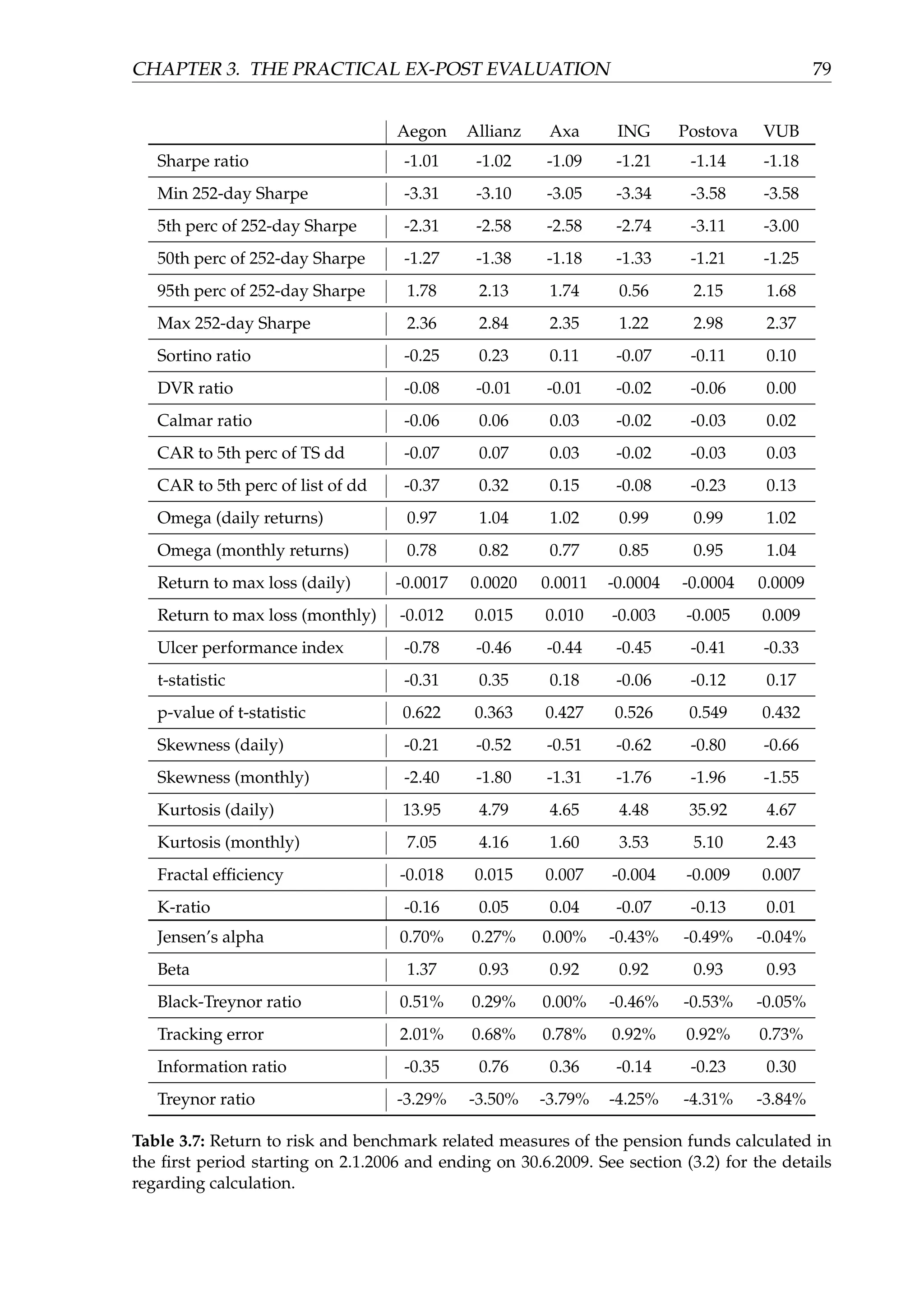
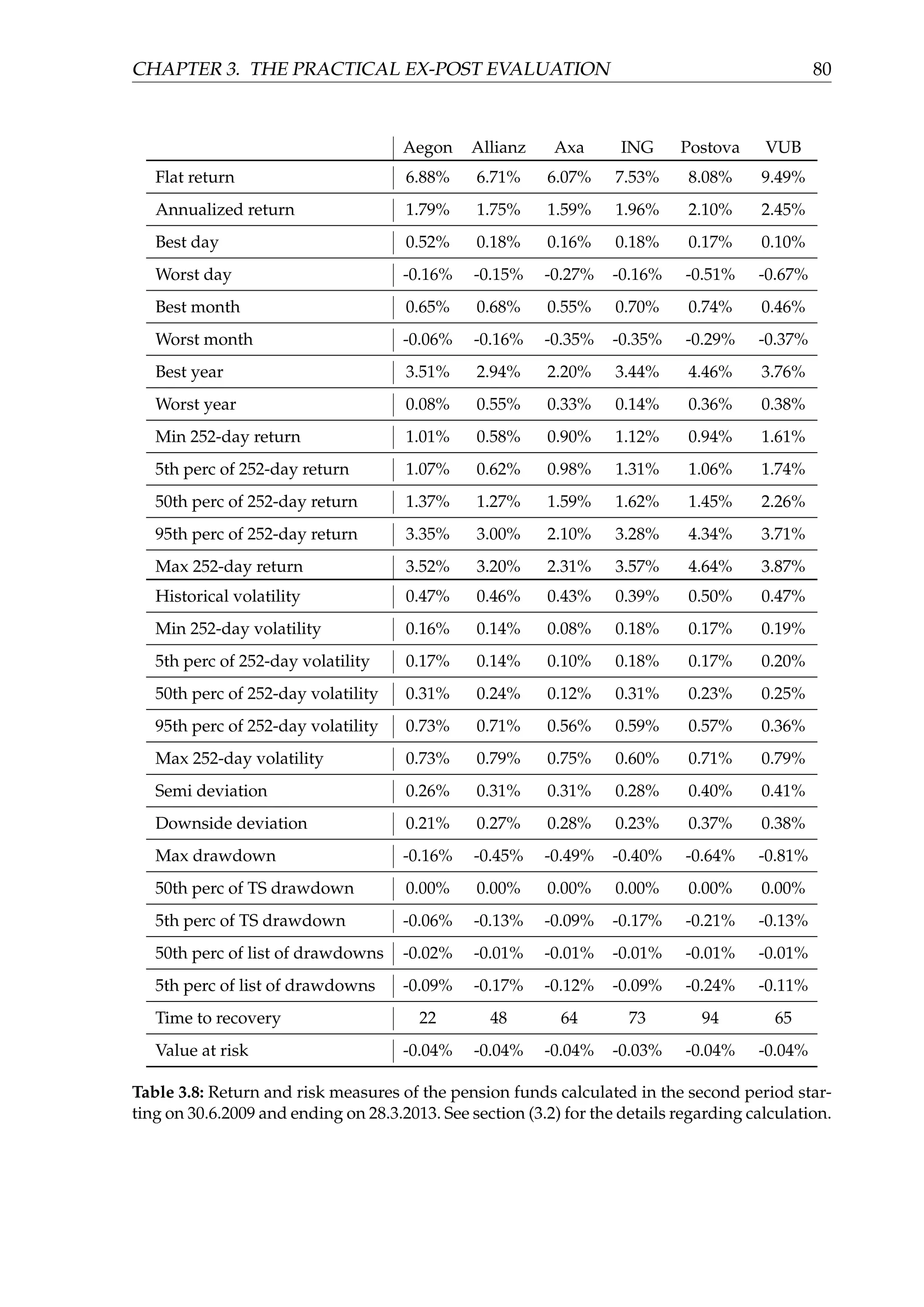
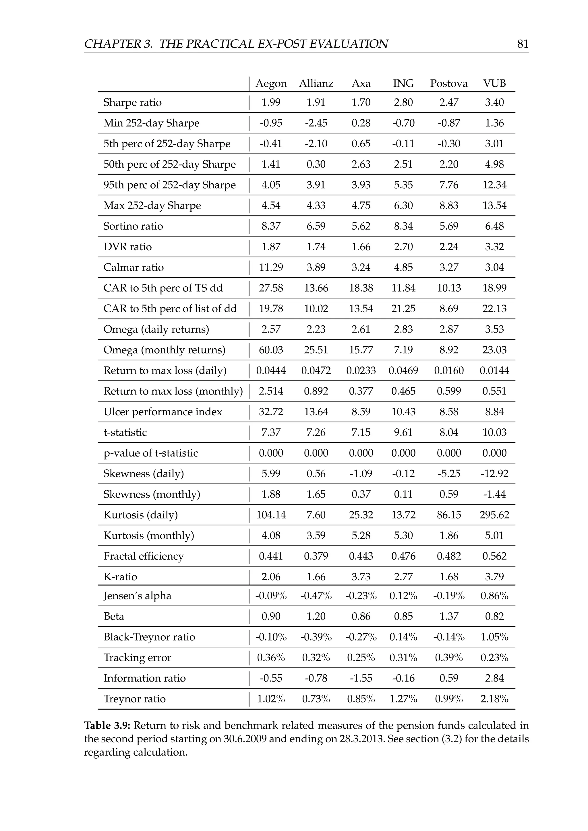
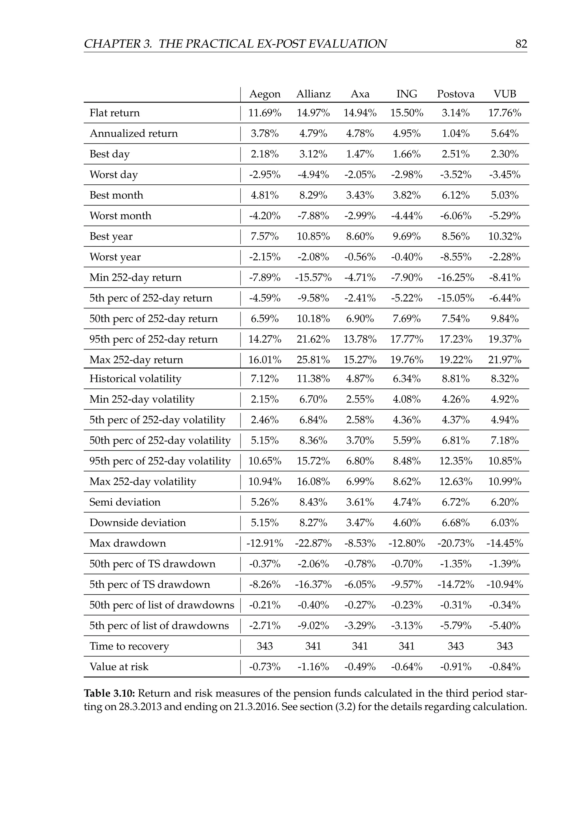
54. Chapter 3
The practical ex-post evaluation
We will demonstrate, analyze and compare all of the measures from the chapter (2) for
the six equity funds managed by six different pension companies of the Slovak funded
pillar (defined contribution) pension system. We have chosen the Slovak funded pillar
(DC) pension system funds for several reasons. Firstly, an author has already been
involved in the DC pension research, see for example [26], [27] or [28]. Secondly, the
funds in the funded pillar employ a quite similar strategy in managing their assets1
,
therefore they constitute a good peer group. They also now have a track record of more
than ten years of managing pension assets. Furthermore, the number of six (funds) is
very well suited for the purposes of this analysis. It is enough to uncover differences
and hence demonstrate measures from this paper and on the other hand it is not too
extensive to exhaust a reader. Last but not least, an author’s current occupation is
not related to the Slovak funded pillar at all and therefore the analysis should not be
biased because of any potential conflict of interests.
The reason why we have chosen the equity fund category is pretty straightforward.
The guaranteed bond fund, and the non-guaranteed equity fund are now the only two
funds which pension companies are obliged to manage. Hence, our choice has been
narrowed to the two options, of which we have chosen for the purposes of our analysis
the equity funds because of their higher diversity and less strict legal limits.
3.1 The funded pillar of the Slovak pension system
3.1.1 Brief history
Until 2005, Slovakia employed only a compulsory Pay As You Go (PAYG) pension sys-
tem. In simplicity, the system was, and still is, based on the pension payments to the
current pensioner’s being paid out of the wages of the currently working population.
1
By „quite similar” we mean a long term strategy with a mandate of creating a pension income for a
pensioner in the long run. Of course we are aware of the fact that the strategies may differ substantially
in carrying out this mandate.
49

55. CHAPTER 3. THE PRACTICAL EX-POST EVALUATION 50
That, naturally, has raised questions about sustainability of such a system, should the
population age rapidly (which happens to be the case). Hence, the pension reform
from 2005 introduced two additional pillars - the mandatory (for new savers) defined
contribution scheme (funded pillar) and the voluntary defined contribution scheme
(third pillar). The PAYG system (first pillar) remained managed by the government,
whereas the other two pillars have begun to be managed by the private pension com-
panies via pension funds.
During 2005-2008 each pension company in the funded pillar managed three funds
- conservative, balanced and growth fund with relatively free investment mandate and
not so strict legal limits. After the crisis of 2008, the Slovak government ratified an
amendment to the pension law, which made it compulsory for the pension companies
to evaluate performance of all of their funds on a rolling 6-month basis. In case of any
loss on any 6-month horizon, the pension company was obliged to compensate such a
loss to the pensioners out of their own capital. This resulted into highly conservative
investment strategies of all of the funds, where the majority of portfolios consisted of
term deposits and short term bills.
Another amendment of the pension law from 2011 canceled the guaranty of not
making a loss on any 6-month horizon in all of the funds except the conservative
(bond) fund, where the guaranty was changed from the 6-month horizon to the 5-year
horizon. The pension companies were also obliged to start managing four funds with
the new names - the bond fund, the mixed fund, the equity fund and the index fund.
This amendment had not resulted into any material changes in investment strategies
of the pension companies, because another amendment of the law was supposed to be
ratified a year later.
3.1.2 Current setup of the pillar
Based on the amendment of the pension law from August 2012, each pension company
is now obliged to manage at least two funds - the guaranteed bond fund and the non-
guaranteed equity fund, while any additional funds are voluntary. In the guaranteed
bond fond a pension company is now obliged by law to compensate any loss made on
any rolling 10-calendar year period to pensioners from its own capital. In other funds,
no guaranty has been imposed by the law. This finally resulted into huge changes of
the investment strategies employed in all of the funds. Majority of the funds have
increased their risk with an aim of increasing a potential long term return).
3.2 Description of the measures and data
3.2.1 Fund data
We obtained the daily price data for the six equity funds managed by six pension
companies (in the alphabetical order of the pension company):

56. CHAPTER 3. THE PRACTICAL EX-POST EVALUATION 51
• Vital, non-guaranteed equity fund of Aegon,
• Progres, non-guaranteed equity fund of Allianz,
• Akciovy, non-guaranteed equity fund of Axa,
• Profit, non-guaranteed equity fund of ING,
• Prosperita, non-guaranteed equity fund of DSS Postovej banky (our abbreviation
- Postova) and
• Profit, non-guaranteed equity fund of VUB Generali (our abbreviation - VUB).
The data was obtained from the web pages of the pension companies (in case they
provided it)2
or from the web page www.manazeruspor.sk in case of Aegon and Allianz.
The data was normalized to the base value of 1 according to (2.2) as of 2.1.2006 and
ends on 21.3.2016. The dates of the data were aligned to one of the shortest time series,
the ING’s fund, to avoid repeating values.3
The price data of the funds prior to 1.1.2009
(abandonment of the Slovak koruna and introduction of the euro) have been already
adjusted in our data source according to the official conversion rate. The data for the
risk free rate represented by the 3-month Euribor were obtained from Bloomberg.
3.2.2 Performance measures
We calculated the performance measures for each fund for the four different examina-
tion periods:
1. the whole sample 2.1.2006-21.3.2016,
2. the first part of the sample, 2.1.2006-30.6.2009, during which the pension compa-
nies were not obliged to guarantee a profit; this includes the financial crisis,
3. the second part of the sample, 30.6.2009-28.3.2013, during which the pension
companies were obliged to guarantee a profit on a rolling 6-calendar month basis
and hence invested very conservatively
2
https://www.vubgenerali.sk/dochodkove-fondy/vykonnost-dochodkovych-fondov,
https://dss.nn.sk/fondy/dynamika-akciovy-negarantovany-d-f/historicky-vyvoj-hodnot-
dochodkovych-jednotiek/, http://www.dsspabk.sk/dochodkove-fondy/prosperita/,
https://www.axa.sk/produkty/dochodok/aktualne-informacie-dochodkovych-fondov/aktualne-
hodnoty-fondov/obsah/ii-pilier/
3
There happen to be some dates in the sample, on which certain pension companies do provide the
price data and some do not. In case there is some missing price data on a certain date (aligned to the
aforementioned ING’s time series) for some fund, the last available price data point is used instead.
That is, there may be some repeating values for some funds. This is also the reason why we align to the
shortest instead of to the longest time series.

57. CHAPTER 3. THE PRACTICAL EX-POST EVALUATION 52
4. and finally the third part of the sample, 28.3.2013-21.3.2016 during which the
pension companies started to again invest in line with their long term capital
appreciation mandate, because of the missing capital protection requirements.
For the sake of a better readability in the tables below we use the names of the measu-
res instead of their official abbreviations defined in chapter (2). This is the description
of all of the analyzed measures:
• Calendar year returns - these are the simple yearly returns from the section (2.1.4)
for a year i starting on the close of the last day of the year (i − 1) and ending on
the close of the last day of the year i; an exception is the year 2006, where the
calculation starts on the close of 2.1.2006 and the year 2016 where the calculation
ends on the close of 21.3.2016
• Flat return - simple return for the whole period under examination from (2.1)
• Annualized return - cumulative annual growth of return based on trading days
from (2.4)
• Best/worst day/month/year - based on the flat return for the calendar days/months/years;
in case the month (year) in the sample under examination has not ended yet (for
example in 2016 we have only the data up to and including 21.3.2016), the month
to date (year to date) figure is used (flat, not annualized)
• Xth perc of 252-day return - the percentile of the rolling 252-trading day return
from (2.5)
• Historical volatility - the annualized historical volatility from (2.7)
• Xth perc of 252-day volatility - the percentile of the rolling 252-trading day annu-
alized historical volatility from (2.8)
• Semi deviation - the annualized historical semi deviation from (2.9)
• Downside deviation - the annualized historical downside deviation from (2.10)
with MAR = 0
• Max drawdown - the maximum drawdown from (2.13)
• Xth perc of TS drawdown - the percentile of the time series of the drawdown from
(2.14)
• Xth perc of list of drawdowns - the percentile of the list of local maximum drawdo-
wns from (2.16); also the drawdown on the last day in the sample, that is not yet
ended drawdown, is included into the calculation
• Time to recovery - maximum time to recovery in days from (2.18)

58. CHAPTER 3. THE PRACTICAL EX-POST EVALUATION 53
• Value at risk - daily 95% Value at Risk from (2.20)
• Sharpe ratio - the annualized Sharpe ratio from (2.22) with the risk free rate equal
to the average of the 3-month Euribor over the specific period under inspection
• Xth perc of 252-day Sharpe - the percentile of the rolling 252-trading day annuali-
zed Sharpe ratio from (2.23)
• Sortino ratio - the annualized Sortino ratio from (2.25) with MAR = 0
• DVR ratio - the DVR ratio from (2.26)
• Calmar ratio - the Calmar ratio from (2.28)
• CAR to 5th perc of TS drawdown - the cumulative annualized trading day return
to 5th percentile of the time series of the drawdown from (2.29)
• CAR to 5th perc of list of dd - the cumulative annualized trading day return to 5th
percentile of the list of local maximum drawdowns from (2.30)
• Omega (daily/monthly returns) - the Omega ratio from (2.31) calculated from the
daily/monthly returns with MAR = 0
• Return to max loss (daily/monthly) - return to maximal loss calculated from the
daily/monthly returns from (2.32)
• Ulcer performance index - Ulcer performance index from (2.33) with the risk free
rate equal to the average of the 3-month Euribor over the period under inspec-
tion
• t-statistic - the one-sided Student’s t-test test statistic for the hypothesis
H0 : µ ≤ MAR vs. H1 : µ > MAR , where µ is the daily return over the period
under inspection and MAR = 0 from (2.36)
• p-value of t-statistic - p-value for the one-sided t-test of the above mentioned hy-
pothesis
• Skewness (daily/monthly) - the skewness of the daily/monthly returns from (2.38)
• Kurtosis (daily/monthly) - the kurtosis of the daily/monthly returns from (2.39)
• Fractal efficiency - the fractal efficiency from (2.40)
• K-ratio - the K-ratio from (2.42)
There is not any specific benchmark for the equity pension funds in the funded
pillar. It is also impossible to benchmark the whole 10-year period with a uniform
benchmark, because of the significant changes in the investment policies induced by
the changes in the pension law. Therefore, we decided to create our own artificial

59. CHAPTER 3. THE PRACTICAL EX-POST EVALUATION 54
benchmark. The benchmark is the daily average of returns of all of the funds under
inspection. We are aware of the fact that when we create a benchmark this way, it is
impossible for all of the funds to beat the benchmark. We are also aware that this may
distort the regression analysis, because we will be regressing a fund’s returns on the
benchmark which already contains, among other, also the fund’s returns. In spite of
this we will use this benchmark because we believe it remains one of the most fair and
simple ways of constructing the benchmark for the purposes of our analysis.
The benchmark related measures are calculated from the weekly, instead of the
daily returns to reduce the noise. See also section (2.5) and footnote (22) for more
thorough explanation.
• Jensen’s alpha - the annualized Jensen’s alpha from (2.44) with the risk free rate
equal to the 3-month Euribor during the period under inspection and the bench-
mark described in the paragraph above
• Beta - the beta against the benchmark from section (2.5.1)
• Black-Treynor ratio - the annualized Black-Treynor ratio from (2.45)
• Tracking error - the annualized tracking error from (2.47)
• Information ratio - the information ratio from (2.48)
• Treynor ratio - the Treynor ratio from (2.49)
3.3 Evaluation
We will firstly perform a visual analysis of the Slovak pension funds’ performance.
Next, we will continue by examining the return measures, risk measures, return to
risk measures and benchmark related measures for the whole sample. An analysis of
the first part of the sample containing the financial crisis in 2008 will follow. The next
two sections will deal with the analysis of the second and third, most recent, part of
the sample. The last section will briefly comment on criteria difficult to measure.
3.3.1 Visual Evaluation
Firstly, we perform a visual analysis of the Slovak pension funds’ performance which
is carried out in the charts (3.1)-(3.10). The equity curves and the time series of the dra-
wdown are charted for all funds. Rolling return, volatility, Sharpe ratio, Value at Risk
and the return distribution is charted only for the VUB equity fund, with the aim of
not exhausting a reader. Nonetheless, the character of the figures (not reported here)
containing the aforementioned measures depicted only for the VUB fund is quite si-
milar for all of the funds in our analysis.

60. CHAPTER 3. THE PRACTICAL EX-POST EVALUATION 55
Ae Al Ax In Pb
Al 0.77
Ax 0.90 0.86
In 0.82 0.87 0.87
Pb 0.83 0.80 0.85 0.75
Vu 0.87 0.84 0.91 0.80 0.90
(a) 2.1.2006 - 21.3.2016
Ae Al Ax In Pb
Al 0.82
Ax 0.83 0.95
In 0.81 0.88 0.89
Pb 0.71 0.75 0.76 0.72
Vu 0.82 0.93 0.94 0.88 0.76
(b) 2.1.2006 - 30.6.2009
Ae Al Ax In Pb
Al 0.12
Ax 0.24 0.61
In 0.28 0.19 0.37
Pb 0.18 0.34 0.37 0.23
Vu 0.29 0.17 0.26 0.20 0.63
(c) 30.6.2009 - 28.3.2013
Ae Al Ax In Pb
Al 0.81
Ax 0.93 0.90
In 0.83 0.89 0.87
Pb 0.89 0.81 0.90 0.77
Vu 0.92 0.83 0.94 0.80 0.92
(d) 28.3.2013 - 21.3.2016
Table 3.1: Correlation of the daily returns among the Slovak funded pillar equity pension funds
for the different calculation periods. Row and column names denote the pension companies
which manage the funds (Ae=Aegon, Al=Allianz, Ax=Axa, In=Ing, Pb=Postova, Vu=VUB).
Data source and normalization: see section (3.2.1).
Figure (3.1) depicts (in two parts, for the sake of clarity) the daily equity curves of
the six equity funds in the whole, more than 10 year long, sample. We can see that the
evolution of the wealth in each fund was quite similar. Correlation among the funds’
returns is high. For example the average correlation of the daily returns among funds
for the whole sample is 0.84, see table (3.1). We calculated also the average correlation
of the weekly returns to mitigate any potential impact in the delay of the pricing of
the funds.4
The weekly correlation was even higher, 0.9 for the whole sample, see
table (3.2).
4
Recall that illiquidity of some securities in the portfolios may cause differences in funds’ returns
on a daily basis. Consider an example of a local covered bond which may be repriced only when the
trade on the exchange is made. The main, liquid bond market may experience significant moves which
are priced on a daily basis but the covered bond will be repriced only after the next trade. Hence,
if one fund possess the bond which was not traded after the market movement and the other fund
possess another bond which, however, was traded after the movement, the pricing of the funds may be
different, although the economical exposure remains the same for both funds. This potential difference
should, however, be smoothed when using lower frequency returns.

61. CHAPTER 3. THE PRACTICAL EX-POST EVALUATION 56
Ae Al Ax In Pb
Al 0.86
Ax 0.92 0.91
In 0.89 0.88 0.91
Pb 0.87 0.92 0.89 0.86
Vu 0.89 0.94 0.95 0.90 0.92
(a) 2.1.2006 - 21.3.2016
Ae Al Ax In Pb
Al 0.91
Ax 0.89 0.97
In 0.89 0.94 0.94
Pb 0.90 0.94 0.93 0.92
Vu 0.90 0.97 0.97 0.94 0.94
(b) 2.1.2006 - 30.6.2009
Ae Al Ax In Pb
Al 0.21
Ax 0.24 0.68
In 0.36 0.25 0.32
Pb 0.16 0.46 0.38 0.29
Vu 0.48 0.41 0.32 0.36 0.47
(c) 30.6.2009 - 28.3.2013
Ae Al Ax In Pb
Al 0.94
Ax 0.94 0.96
In 0.91 0.89 0.91
Pb 0.92 0.93 0.91 0.86
Vu 0.94 0.95 0.97 0.89 0.92
(d) 28.3.2013 - 21.3.2016
Table 3.2: Correlation of the weekly returns among the Slovak funded pillar equity pen-
sion funds for the different calculation periods. Row and column names denote the pension
companies which manage the funds (Ae=Aegon, Al=Allianz, Ax=Axa, In=Ing, Pb=Postova,
Vu=VUB). Data source and normalization: see section (3.2.1).
We may also observe the three entirely different regimes in the investment policies
employed by the funds. The first part of the sample, during which the pension compa-
nies were not obliged to compensate loss to pensioners, but were still subject to strict
legal limits. Next, the second part, when the pension companies invested very conser-
vatively to avoid any loss on a 6-month rolling horizon. Finally, the third part, when
the pension companies were allowed by policymakers to invest the most aggressively
so far.
Upper part of the figure (3.2) depicts the daily equity curves of the six equity funds
in the first part of the sample spanning approximately three and a half years. This
includes the final months of the equity market boom, that is 2006 and first half of 2007,
as well as the financial crisis of 2008. We can see that all of the funds experienced
material losses and substantially elevated volatility during the crisis.
Lower part of the figure (3.2) displays the equity curves of the funds in the second
part of the sample spanning approximately three years and nine months. This period
was strongly influenced by the amendment of the pension law which made it compul-
sory for the pension companies to guarantee a rolling 6-calendar month nonnegative
performance for pensioners. In case of not fulfilling this guaranty, the pension com-
pany was obliged to compensate a pensioner any loss from the company’s own capi-
tal. It resulted into the portfolios consisting only of very low duration bonds, money
market instruments and term deposits. This translated into very smooth equity curves.

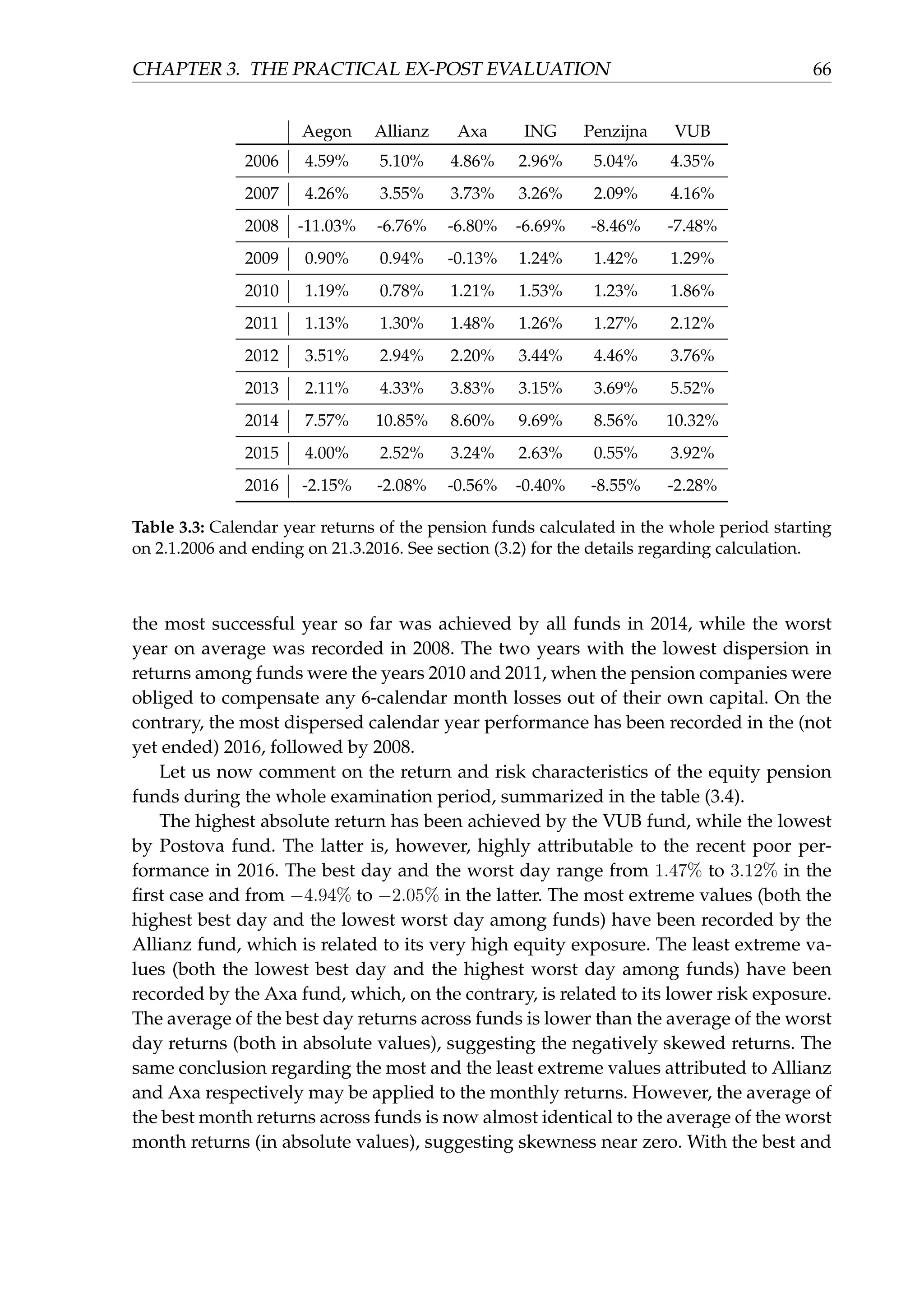
62. CHAPTER 3. THE PRACTICAL EX-POST EVALUATION 57
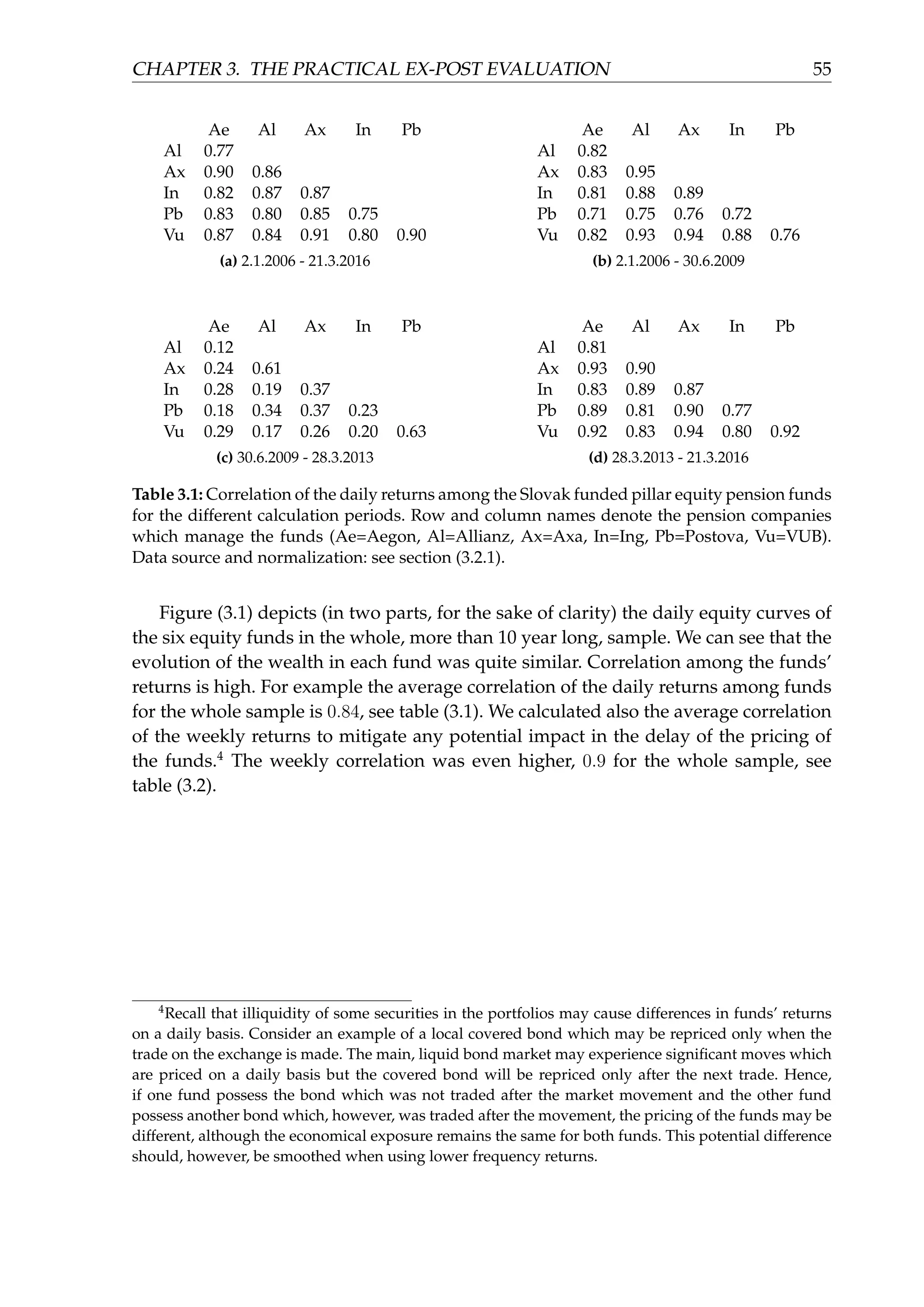
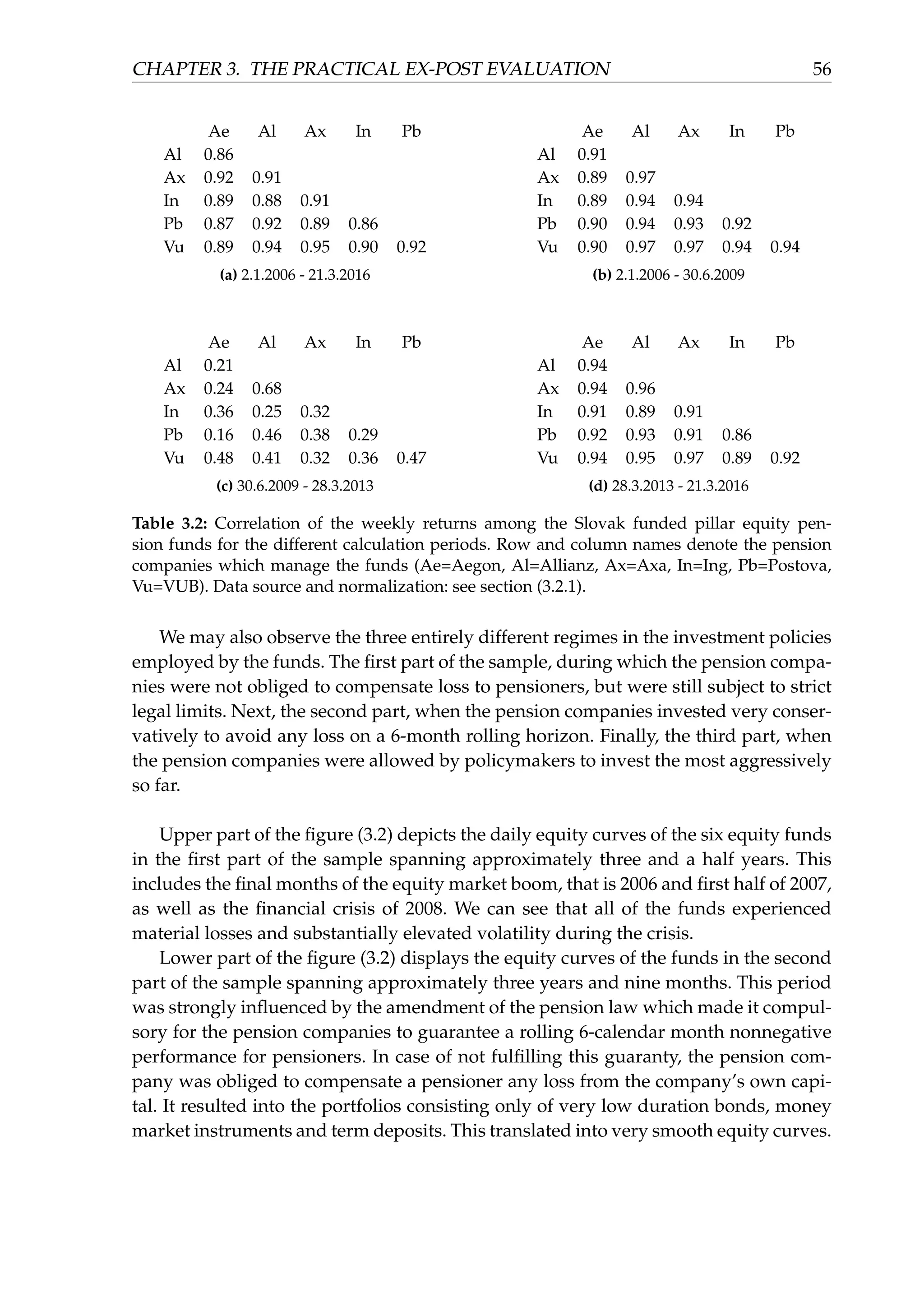
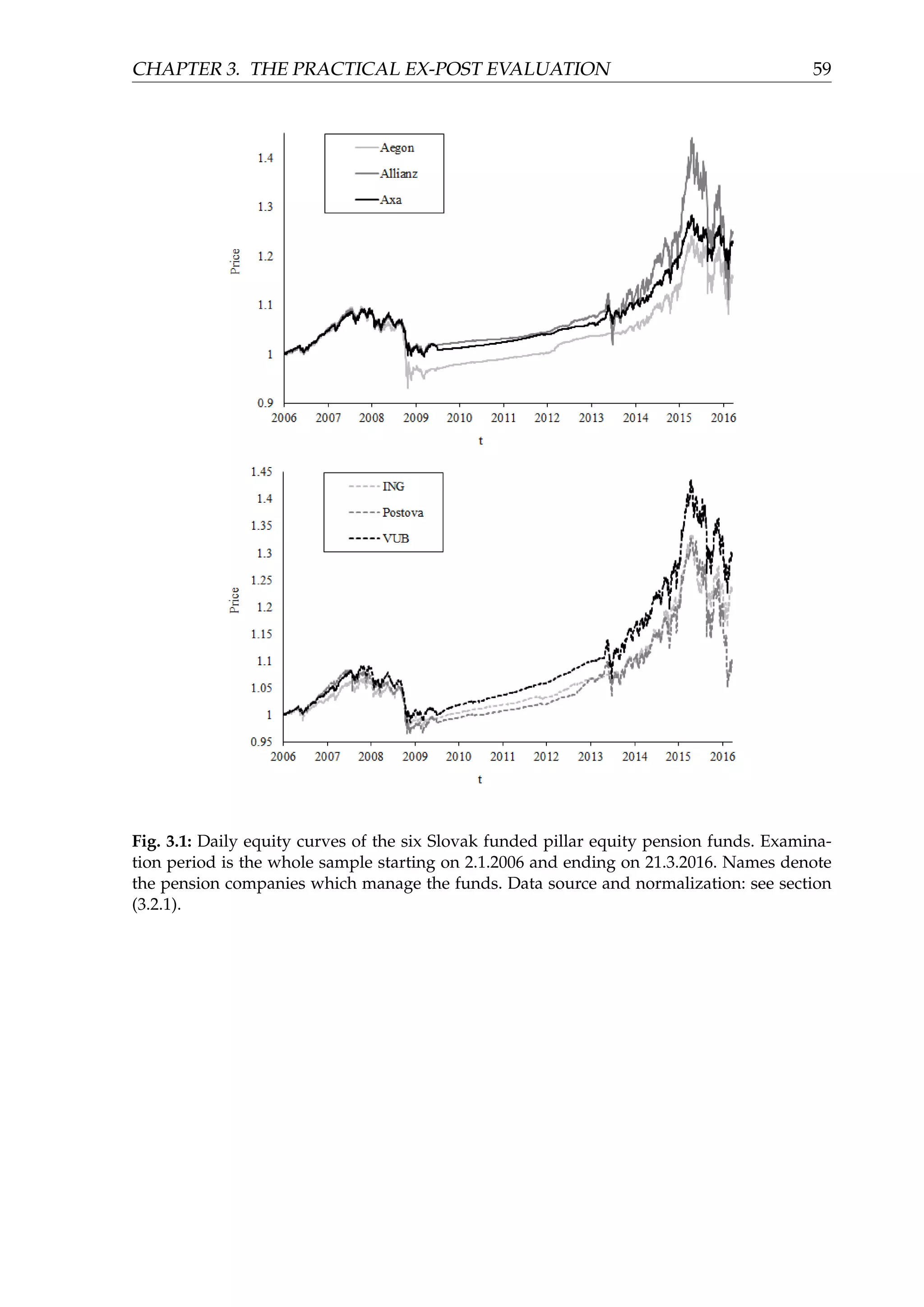
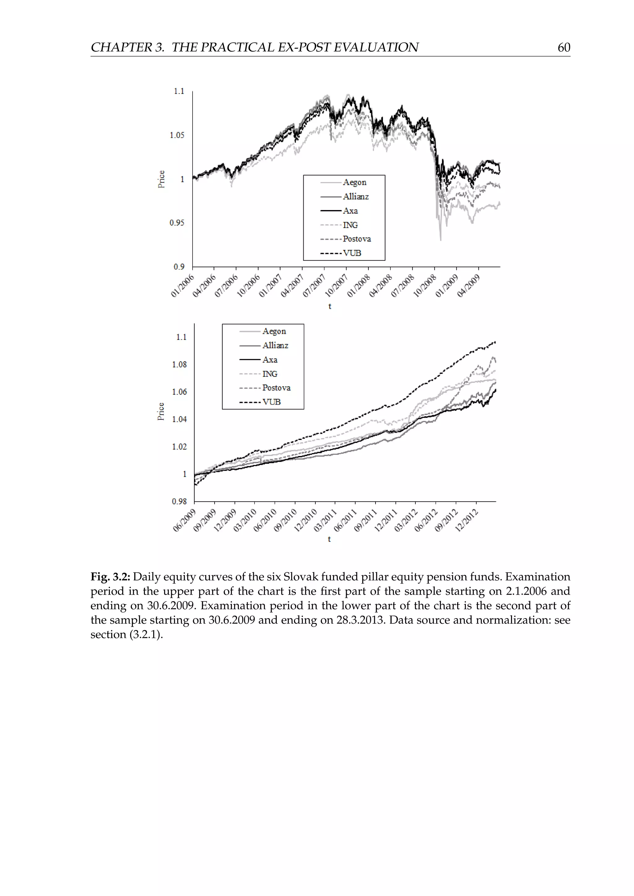
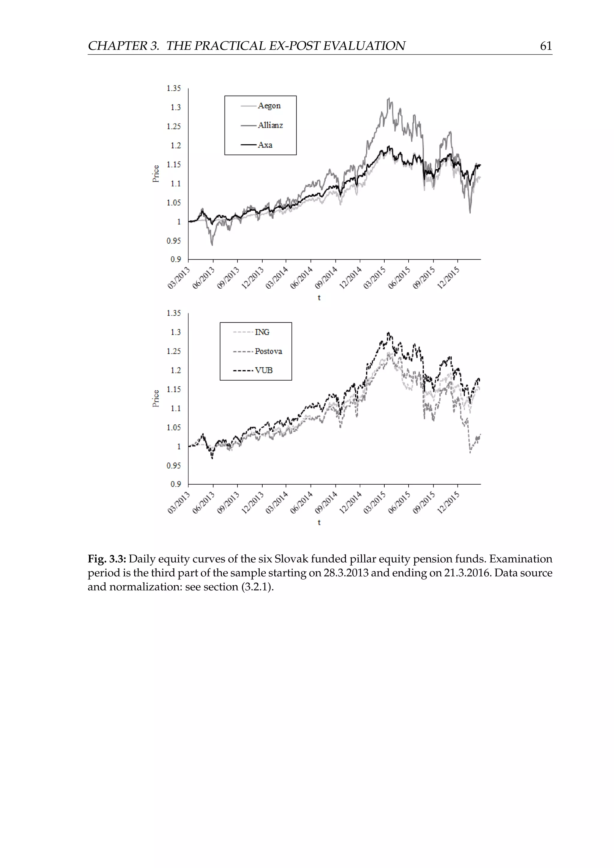
Figure (3.3) depicts (in two parts, for the sake of clarity) the equity curves of the
funds in the third part of the sample spanning approximately three most recent years.
We can observe that the pension companies started to again invest more aggressively
with a substantial exposure to equity markets. This is the result of the amendment of
the pension law which canceled the guaranty obligation for the equity funds.
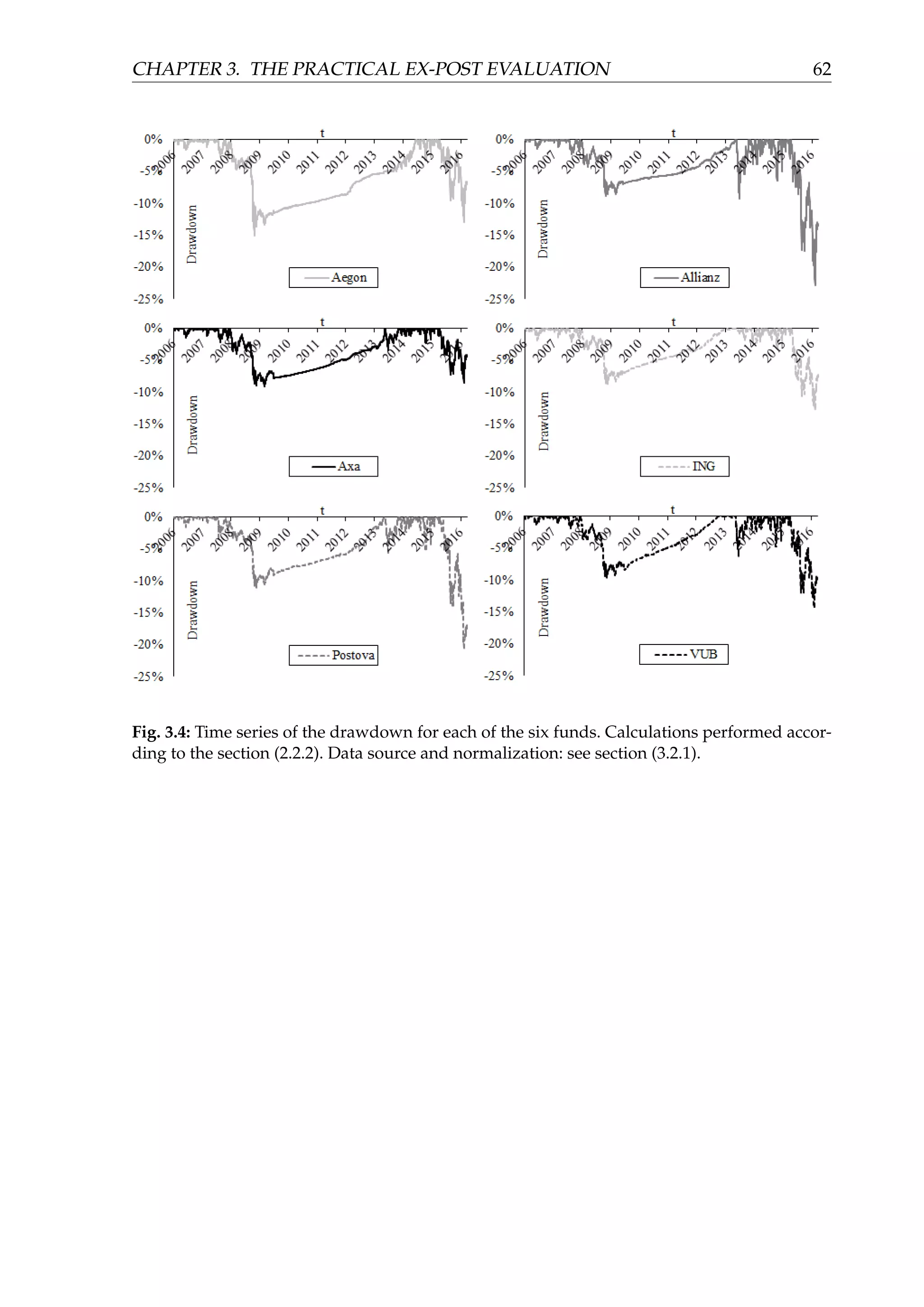
Figure (3.4) displays the daily time series of the drawdown for each fund. The cri-
sis of 2008 caused the funds to experience drawdowns from −9% to −15%. It then
took the funds more than 5 years (with an exception of VUB, in which case a little less
than 5) to recover this drawdown and create the new maximum value of the fund.
Another volatile period accompanied with high drawdowns happened very recently
in 2016 and culminated in February. Several funds experienced their new maximum
drawdown and neither fund has recovered this drawdown yet, as of 21.3.2016.
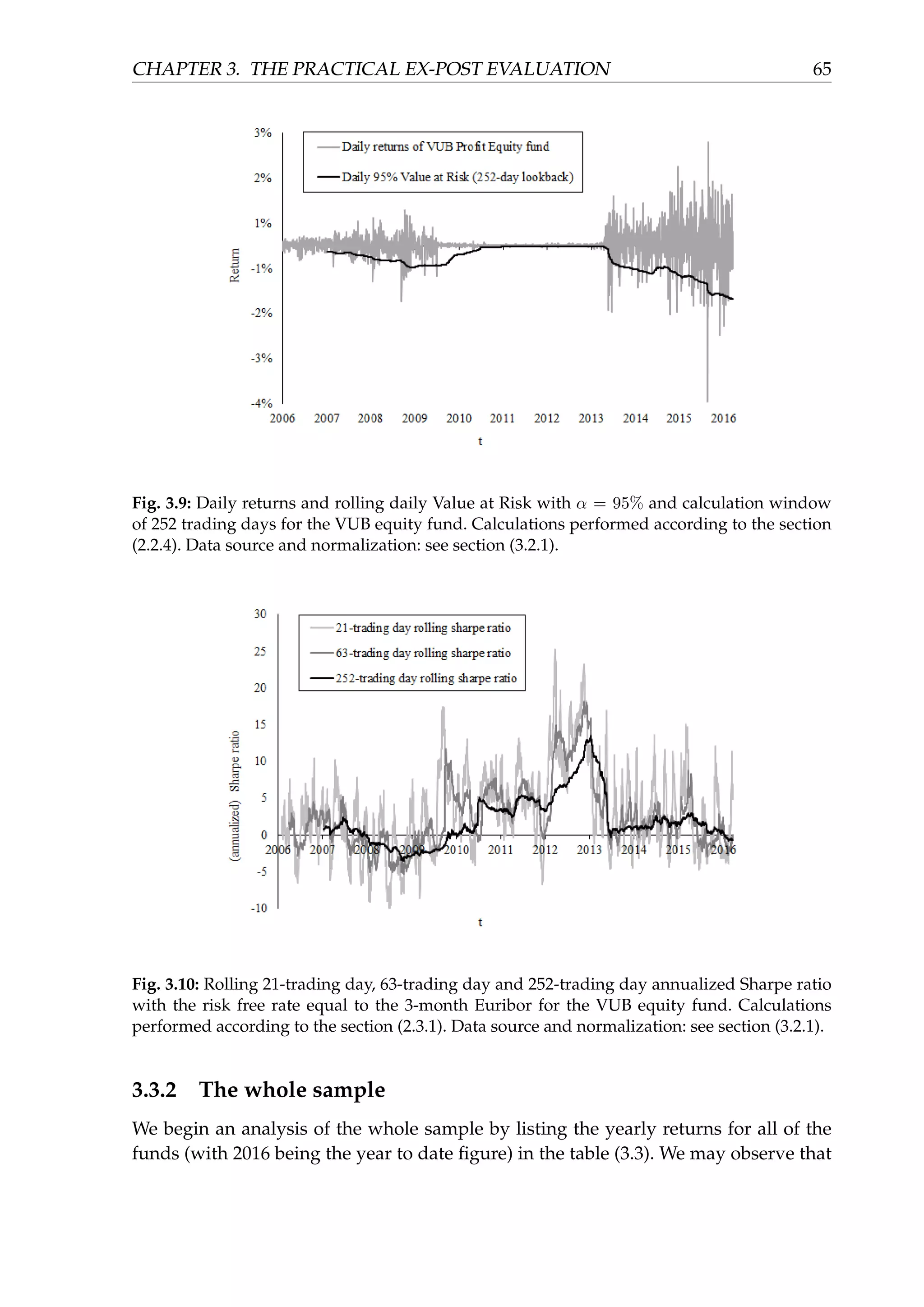
Figure (3.5) depicts the rolling 21-trading day, 63-trading day and 252-trading day
simple return of the VUB equity fund. We may notice swings ranging from −10% to
more than 20% when 252-day return is considered, especially in the first and the third
part of the sample. The second part of the sample is characterized by very stable re-
turns.
Chart (3.6) helps to analyze the distribution of the daily returns of the VUB equity
fund for the whole sample. It contains the histogram of the aforementioned returns.
The most frequent bin with more than 40% of the observations belongs to the inter-
val (0%, 0.1%]. We may also observe high kurtosis and a slight, hardly recognizable
skewness.
The same statements may be applied to the monthly distribution of the returns of
the VUB equity fund, which are depicted in the figure (3.7).
Figure (3.8) displays the rolling 21-trading day, 63-trading day and 252-trading day
annualized historical volatility of the VUB equity fund. We may notice three distinct
periods corresponding with the pension law amendments as mentioned several times
earlier. Volatility in the first period peaked during the financial crisis and the collapse
of the Lehman Brothers. However, it was still low when compared to the long-term
pension funds managed in the developed countries, where their volatility approaches
equity volatility (usually more than 10% p.a.). In the second period, when the pension
companies were obliged to compensate any 6-month losses, the volatility was abnor-
mally low (ranging between 0.15% p.a. and 0.4% p.a.). This is the result of the low risk
investments made by fund managers at that time. In the third period, when the ob-
ligations to compensate losses ceased to exist, the volatility increased to its historical
maximum. This is in line with a higher risk (equity) exposure of the fund.
Rolling daily Value at Risk with 252-day calculation window and α = 95% confi-

63. CHAPTER 3. THE PRACTICAL EX-POST EVALUATION 58
dence level is charted in the figure (3.9). It has a similar character as the figure (3.8),
that is, moderate risk in the first period, very low risk in the second period and high
risk in the third period.
Figure (3.10) depicts the rolling 21-trading day, 63-trading day and 252-trading day
annualized Sharpe ratio of the VUB equity fund with the risk free rate of 3-month Euri-
bor. We again observe the three distinct periods corresponding to the already menti-
oned amendments of the pension law. The first period was also substantially affected
by the financial crisis. We may observe that the rolling 252-day Sharpe ratio plunged
to its historical low in 2008. Contrary to it, in the next period (2009-2013) the 252-day
Sharpe ratio firstly increased to approximately 5 and then climbed even higher to cre-
ate the historical maximum of more than 10.
Such value of the Sharpe ratio is typically unrealistic and almost unattainable for
common pension funds. These funds have high exposure to risky assets, in order to
increase their long-term return potential. However, in case of the pension funds in
Slovakia during the aforementioned period, the rationale behind such Sharpe ratio is
pretty straightforward. Majority of the assets bought by the portfolio managers had a
volatility close to 0, because of their short maturity and low risk. Consider also term
deposits, which, by definition, have 0 volatility, but of course only in case that the
institution where the deposit is made does not default. If it does not, and their return
exceeds the return of the risk free rate, they have a property of an infinite Sharpe ratio.
All of these instruments helped volatility of the fund approach 0, whereas their return
spread over the risk free rate of the 3-month Euribor was still high over that period.
This resulted into very high Sharpe ratios.
The most recent period shows the most realistic picture of the behavior of the equ-
ity pension fund portfolios. That is, 1-year Sharpe ratios in between the range of app-
roximately -3 and 3.

64. CHAPTER 3. THE PRACTICAL EX-POST EVALUATION 59
Fig. 3.1: Daily equity curves of the six Slovak funded pillar equity pension funds. Examina-
tion period is the whole sample starting on 2.1.2006 and ending on 21.3.2016. Names denote
the pension companies which manage the funds. Data source and normalization: see section
(3.2.1).

65. CHAPTER 3. THE PRACTICAL EX-POST EVALUATION 60
Fig. 3.2: Daily equity curves of the six Slovak funded pillar equity pension funds. Examination
period in the upper part of the chart is the first part of the sample starting on 2.1.2006 and
ending on 30.6.2009. Examination period in the lower part of the chart is the second part of
the sample starting on 30.6.2009 and ending on 28.3.2013. Data source and normalization: see
section (3.2.1).

66. CHAPTER 3. THE PRACTICAL EX-POST EVALUATION 61
Fig. 3.3: Daily equity curves of the six Slovak funded pillar equity pension funds. Examination
period is the third part of the sample starting on 28.3.2013 and ending on 21.3.2016. Data source
and normalization: see section (3.2.1).

67. CHAPTER 3. THE PRACTICAL EX-POST EVALUATION 62
Fig. 3.4: Time series of the drawdown for each of the six funds. Calculations performed accor-
ding to the section (2.2.2). Data source and normalization: see section (3.2.1).

68. CHAPTER 3. THE PRACTICAL EX-POST EVALUATION 63
Fig. 3.5: Rolling 21-trading day, 63-trading day and 252-trading day simple return of the VUB
equity fund. Calculations performed according to the section (2.1.3). Data source and norma-
lization: see section (3.2.1).
Fig. 3.6: Empirical distribution (histogram) of the daily returns of the VUB equity fund. The
−1.5% bin represents returns from the interval (−∞, −0.015] and for example the 1% bin re-
presents returns from the interval (0.009, 0.01]. Similarly for other bins. Data source and nor-
malization: see section (3.2.1).

69. CHAPTER 3. THE PRACTICAL EX-POST EVALUATION 64
Fig. 3.7: Empirical distribution (histogram) of the monthly returns of the VUB equity fund.
The −3% bin represents returns from the interval (−∞, −0.03] and for example the 2% bin
represents returns from the interval (0.015, 0.02]. Similarly for other bins. Data source and nor-
malization: see section (3.2.1).
Fig. 3.8: Rolling 21-trading day, 63-trading day and 252-trading day annualized historical vo-
latility of the VUB equity fund. Calculations performed according to the section (2.2.1). Data
source and normalization: see section (3.2.1).

70. CHAPTER 3. THE PRACTICAL EX-POST EVALUATION 65
Fig. 3.9: Daily returns and rolling daily Value at Risk with α = 95% and calculation window
of 252 trading days for the VUB equity fund. Calculations performed according to the section
(2.2.4). Data source and normalization: see section (3.2.1).
Fig. 3.10: Rolling 21-trading day, 63-trading day and 252-trading day annualized Sharpe ratio
with the risk free rate equal to the 3-month Euribor for the VUB equity fund. Calculations
performed according to the section (2.3.1). Data source and normalization: see section (3.2.1).
3.3.2 The whole sample
We begin an analysis of the whole sample by listing the yearly returns for all of the
funds (with 2016 being the year to date figure) in the table (3.3). We may observe that

71. CHAPTER 3. THE PRACTICAL EX-POST EVALUATION 66
Aegon Allianz Axa ING Penzijna VUB
2006 4.59% 5.10% 4.86% 2.96% 5.04% 4.35%
2007 4.26% 3.55% 3.73% 3.26% 2.09% 4.16%
2008 -11.03% -6.76% -6.80% -6.69% -8.46% -7.48%
2009 0.90% 0.94% -0.13% 1.24% 1.42% 1.29%
2010 1.19% 0.78% 1.21% 1.53% 1.23% 1.86%
2011 1.13% 1.30% 1.48% 1.26% 1.27% 2.12%
2012 3.51% 2.94% 2.20% 3.44% 4.46% 3.76%
2013 2.11% 4.33% 3.83% 3.15% 3.69% 5.52%
2014 7.57% 10.85% 8.60% 9.69% 8.56% 10.32%
2015 4.00% 2.52% 3.24% 2.63% 0.55% 3.92%
2016 -2.15% -2.08% -0.56% -0.40% -8.55% -2.28%
Table 3.3: Calendar year returns of the pension funds calculated in the whole period starting
on 2.1.2006 and ending on 21.3.2016. See section (3.2) for the details regarding calculation.
the most successful year so far was achieved by all funds in 2014, while the worst
year on average was recorded in 2008. The two years with the lowest dispersion in
returns among funds were the years 2010 and 2011, when the pension companies were
obliged to compensate any 6-calendar month losses out of their own capital. On the
contrary, the most dispersed calendar year performance has been recorded in the (not
yet ended) 2016, followed by 2008.
Let us now comment on the return and risk characteristics of the equity pension
funds during the whole examination period, summarized in the table (3.4).
The highest absolute return has been achieved by the VUB fund, while the lowest
by Postova fund. The latter is, however, highly attributable to the recent poor per-
formance in 2016. The best day and the worst day range from 1.47% to 3.12% in the
first case and from −4.94% to −2.05% in the latter. The most extreme values (both the
highest best day and the lowest worst day among funds) have been recorded by the
Allianz fund, which is related to its very high equity exposure. The least extreme va-
lues (both the lowest best day and the highest worst day among funds) have been
recorded by the Axa fund, which, on the contrary, is related to its lower risk exposure.
The average of the best day returns across funds is lower than the average of the worst
day returns (both in absolute values), suggesting the negatively skewed returns. The
same conclusion regarding the most and the least extreme values attributed to Allianz
and Axa respectively may be applied to the monthly returns. However, the average of
the best month returns across funds is now almost identical to the average of the worst
month returns (in absolute values), suggesting skewness near zero. With the best and

72. CHAPTER 3. THE PRACTICAL EX-POST EVALUATION 67
the worst year, the pattern among funds is less consistent and the results are mixed.
With the minimum and the maximum rolling 252-day return spread of the funds, the
results are similar to the best/worst day, that is, the highest extremes are recorded by
Allianz, while the lowest by Axa. The highest median rolling 252-day return belongs
to VUB (corresponding to the highest absolute return), followed by Postova and ot-
her companies with a little dispersion among them (with an exception of VUB, which
wins by far in this measure). Worth noting is the case of Postova whose absolute re-
turn is worst, however median of the 252-day return is the second best after VUB. This
confirms the aforementioned hypothesis that the return of Postova has been worsened
mainly by the past few months.
The lowest historical volatility, and also the lowest minimum, median and maxi-
mum of the rolling 252-day volatility has been achieved by Axa. This is in line with the
paragraph above. On the other hand, the highest historical volatility and the highest
maximum of the rolling 252-day volatility is attributed to Allianz, while the highest
median 252-day volatility to Postova. This suggests, that the risk of the Allianz fund
may have been increased only recently, but by a high mark, whereas the risk of Postova
has been consistently higher than that of the other funds. The semi deviation and do-
wnside deviation do not reveal any surprising results and their pattern correspond
to that of the historical volatility. Ranking among funds is the same whether we use
historical volatility, semi deviation or downside deviation. The maximum drawdown
ranking among funds also approximately corresponds to the ranking by volatility. The
highest drawdown was recorded by Allianz, recently, and the lowest by Axa (see also
the figure (3.4)). The 50th and the 5th percentile of the time series of the drawdowns
now reveal a different structure. The worst fund in this measure is Aegon, which we
may interpret as more of the time spent in higher drawdowns than for any other fund.
The least negative value for 50th percentile and almost the least negative for the 5th
percentile is, on the contrary, recorded by ING, which suggests their fund spent less
time in drawdowns (or in lower drawdowns) than the other funds. Values for the per-
centile of the list of local maximum drawdowns are markedly lower than values for
the percentile of the time series of the drawdowns. This relates a lot to the drawdown
experienced by the funds in 2008, which took them a long time to recover. This dra-
wdown, therefore, spans a large part of the time series of the drawdown and hence lifts
the median up, whereas in the list of the drawdowns this drawdown is included only
as a single value, not influencing the median markedly. The 5th percentile of the list
of the drawdowns is more in line with the maximum drawdowns or volatility, when
compared among funds. The maximum time to recovery has been suffered during the
sole occasion of the crisis of 2008. We may observe that even for the best fund it took
almost 5 years to recover all of the losses and create a new maximum. For the worst,
it took more than 6 and a half years. Value at Risk is again very much in line with the
maximum drawdown or the historical volatility, that is, lowest for Allianz fund and
highest for Axa.
We will now focus on the risk to return characteristics and benchmark related mea-

73. CHAPTER 3. THE PRACTICAL EX-POST EVALUATION 68
sures of the equity pension funds during the whole examination period, summarized
in the table (3.5).
Not every fund was able to generate the return above the 3-month Euribor during
the whole sample. All of the Sharpe ratios are not high, which is primarily the result
of low absolute returns when compared to the risk free rate. Nevertheless, the highest
Sharpe ratio has been recorded by VUB and the lowest by Postova. The situation is
slightly different if we analyze the distribution of the rolling 252-day Sharpe ratios.
The median is highest for Axa and lowest for Allianz, suggesting higher dispersion
of the Sharpe ratio for example for the VUB fund, which scored the best in the entire
sample Sharpe ratio measure. Minimum rolling 252-day Sharpe ratio value is similar
for all funds, while the maximum varies more significantly, with the clear winner of
VUB. The same applies to the 5th and 95th percentile of the rolling 252-day Sharpe
ratios respectively. The Sortino ratio with minimum acceptable return threshold set to
zero is highest for the Axa fund, followed by ING and VUB, and lowest for Postova.
The reason why this ranking differs from that of created by the Sharpe ratio is that
the risk free rate used in the Sharpe ratio subtracted the substantial portion of the Axa
fund’s return and a less substantial portion of the VUB fund’s return. This caused VUB
to win on the Sharpe ratio but lose on the Sortino ratio.
The price paths of all of the funds were very similar, which we were already able to
observe from the figure (3.1). This translates into the same ranking of the funds based
on the DVR ratio when compared to that based on the Sharpe ratio (R2
for the price
paths of the funds were not very distinct from each other). The ratio of the annualized
return to maximum drawdown, the Calmar ratio, is highest for Axa, followed by VUB
and lowest for Postova. If we, however, analyze the ratio of the annualized return to
the 5th percentile of either the time series of the drawdown or list of the drawdowns,
the highest value is again achieved by VUB and lowest by Postova. The reason behind
this ranking switch is exactly the one we explained in sections (2.3.4) and (2.3.5). More
specifically, the maximum drawdown is just a single point measure and can be hea-
vily influenced by one-off events and outliers, whereas the percentile of the drawdown
should represent the more consistent and stable measure of the tail risk. The Omega
ratio, whether calculated from the daily or the monthly returns is highest for the Axa
and VUB funds, while lowest for the Postova. This is consistent with several aforemen-
tioned measures. The return to maximal loss ratio has the same disadvantage as the
Calmar ratio, because its denominator consists of a single point measure, which can
be highly sensitive to outliers. The ranking of the funds (winner Axa, loser Postova)
reflects exactly this fact, because it is heavily dependent on the worst day/month va-
lue, and less dependent on the average daily/monthly return which has been more
similar across funds. On the measure of the Ulcer performance index scores highest
the VUB fund and Allianz, while lowest Postova, which can be mostly attributed to
not outperforming the 3-month Euribor and thus earning a negative numerator in the
measure.
When analyzing the statistical significance of the daily returns of the funds, we

74. CHAPTER 3. THE PRACTICAL EX-POST EVALUATION 69
have come to the conclusion that not every fund was able to record the return signifi-
cantly greater than zero. Only the funds of Axa, ING and VUB were able to generate
the statistically significant return on the 10% and 5% level of significance and no fund
was able to achieve a statistically significant return on the 1% level of significance. The
t-statistic was highest for the Axa fund. The analysis above suggests that the returns
of the funds may be negatively skewed, as consistent with the standard equity market
behavior. Indeed, the skewness of either daily or monthly returns for all of the funds
is negative. The most (least) negative value was recorded by Aegon (ING) for mont-
hly and Postova (Aegon) for daily skewness. The pattern among funds, however, is
not so clear as with several other measures. Kurtosis for all of the funds is much hig-
her than kurtosis of the standard normal distribution, both on the daily as well as the
monthly frequency. The only fund which was able to approach kurtosis of the normal
distribution was the fund managed by Axa with its monthly returns. On the fractal
efficiency measure, the highest value was recorded by Axa and the lowest by Postova.
In terms of the linearity of the returns as measured by the K-ratio, the highest value
was achieved by the VUB fund and the lowest by the Aegon fund.
As we have already explained in the section (3.2.2), our choice of the benchmark
is a synthetic fund created as an average of all of the funds under examination, rather
than the specific index benchmark. This means that, by definition of our construction,
some funds will always be under-performing on a specific measure (with negative,
for example Jensen’s alphas) and some will always be outperforming (with positive,
for example Information ratios). This will depend on their scoring against the average,
that is against the benchmark. Thus, the overall results should be regarded more as the
fund’s ranking against the average rather than as an answer to the question whether
the fund is beating its standard benchmark.
The negative annualized Jensen’s alpha, which may be interpreted as an alpha ver-
sus the average fund, has been recorded by Postova and Aegon, while the highest
Jensen’s alpha has been achieved by VUB. This is closely related to the highest ab-
solute return of the VUB, but does not have to necessarily be so, when we consider
the methodology explained in the section (2.5.1). Moreover, the aforementioned alpha
coefficient was statistically significant at the 5% level only for the VUB fund (p-values
not reported here, are available from the author upon request). The majority of the
funds had the beta close to 1, which had been expected, given the construction of the
benchmark. The slight exceptions are the fund of Allianz with the beta of almost 1.5
and the fund of Axa with, on the contrary, beta of less than 0.7. The beta in this case
can be interpreted as the fund’s sensitivity to the average movement of all of its peer
funds. The results are thus consistent with the previously calculated risk measures,
such as historical volatility, according to which Allianz manages the most risky fund
and Axa the least risky. The beta coefficients were statistically significant on all stan-
dard levels of significance with p-values of the order 10−200
and less (not reported
here and available from the author upon request). The ranking of the funds by the
Black-Treynor ratio is similar to the ranking by the Jensen’s alpha with the exception

75. CHAPTER 3. THE PRACTICAL EX-POST EVALUATION 70
of Axa (second place, thanks to the lower beta), ING (third place) and Allianz (fourth
place). The annualized tracking error against the benchmark has been lowest for the
VUB fund and highest for the Allianz fund. On the measure of the information ratio,
the highest value has been achieved by VUB by a wide margin, followed by the close
values of ING, Allianz and Axa. The lowest information ratio has been achieved by
Postova. Finally, ranking of the funds by the Treynor ratio is identical to the ranking
by the Black-Treynor ratio.
3.3.3 First part of the sample
We will now briefly comment on the return and risk measures of the funds during the
first examination period starting in 2006 and ending in the middle of 2009 listed in the
table (3.6). To not exhaust a reader we will point out only some notable differences.
During the period hit by the financial crisis the returns for all funds were lower
than for the whole sample. Half of the funds recorded negative return (see also the
figure (3.2)). Statistics of the best/worst day/month/year are more consistent across
funds when compared to the entire sample, suggesting pension managers invested
more uniformly. The highest difference between best/worst month/year and also mi-
nimal/maximal 252-day return and the 5th/95th percentile of the 252-day return has
been achieved by Aegon, suggesting the most risky portfolio. The contrary (that is, the
smallest differences) has been recorded by ING.
The historical volatility across funds was much more uniform than during the en-
tire sample and also much lower than the volatility of the typical world pension funds,
suggesting conservative investment policies. The highest dispersion in the distribu-
tion of the volatility (when analyzed via percentiles of the rolling volatility listed in the
table (3.6)) had again the fund managed by Aegon and the lowest the fund managed
by ING. The ranking of the funds based on the semi deviation or the downside de-
viation is identical to that based on the historical volatility. The maximum drawdown
figure ranged from −15.14% for Aegon to −8.86% for ING. The time to recovery has
been similar for all funds, because they had all peaked at approximately the same time
and none of the funds recovered from its drawdown by the end of this period (see also
figure (3.4)).
The main remarks regarding return to risk and benchmark related measures (listed
in the table (3.7)) in the first part of the sample are as follows.
The Sharpe ratio as well as the median Sharpe ratio has been negative far all of
the funds, implying that no fund was able to beat the return of the 3-month Euribor
during the examination period. The distributions of the Sharpe ratios are close to each
other when compared across funds. The DVR ratios are near zero and close to each
other, because of the near zero R2
from the regressions of the funds’ prices against
time. The Calmar ratio has been highest for the Allianz fund, given its highest return
and almost the highest (the least negative) maximum drawdown figure. The same
applies for the ratio of the annualized return against 5th percentile of the drawdown

76. CHAPTER 3. THE PRACTICAL EX-POST EVALUATION 71
(either time series or list of the drawdowns). The Omega ratio calculated from the
daily returns shows very small differences across funds. When calculated from the
monthly returns, VUB achieved the highest value. The Ulcer performance index has
been negative for all funds because of the under-performance against the 3-month
Euribor. Moreover (and not surprisingly), no fund was able to achieve the daily return
significantly greater than zero. The values of the K-ratio and the fractal efficiency are
very low, because of the low returns generated by the funds.
Jensen’s alpha has been surprisingly highest for Aegon (and lowest for Postova),
however none of the alpha coefficients has been statistically significant (p-values not
reported here, are available from the author upon request) at the 10% level (the hig-
hest p-value 0.31). That suggests that the alpha may have been influenced by outliers
and/or the sample may be not large enough. The beta for all of the funds except Ae-
gon has been nearly identical. For Aegon, the higher beta suggests higher risk taking
by the managers. The tracking error has been highest for Aegon, consistent with the
fact that it also ranked top for several other risk measures. The Treynor ratio is highly
negative, because the return on a risk free rate largely exceeded the return generated
by the funds.
To sum up, the performance measures among funds during the period marked by
the financial crisis did not vary notably and they were the worst among our three
chosen sub-parts of the whole sample.
3.3.4 Second part of the sample
We will now briefly comment on the return and risk measures of the funds during
the second examination period starting in the middle of 2009 and ending in the first
quarter of 2013 listed in the table (3.8). This period has been characterized by low risk
portfolios of all funds, because of the legal obligation to compensate losses occurring
on any 6-calendar month rolling period.
Portfolios of the pension funds consisted mainly of short maturity fixed income
assets, such as treasury bills, covered bonds and term deposits. All of the funds achie-
ved to deliver positive returns. This is primarily due to the declining interest rates,
which, naturally, caused the raise in the prices of fixed income securities. Moreover,
no credit events, that is defaults or suspension of interest payments, occurred on the
securities held by the funds. Annualized returns exceeded the risk free rate (0.86% p.a.)
by as low as 0.73% p.a. (Axa) to as high as 1.59% p.a. (VUB). There has not been any
consistent pattern in the best/worst day/month/year among funds that may have
helped to assess the differences in their level of riskiness. The highest differences bet-
ween the minimal/maximal 252-day return and the 5th/95th percentile of the 252-day
return have been recorded by Postova while the contrary (that is, the smallest diffe-
rences) has been recorded by Axa. Volatility and also the distribution of the volatility
has been remarkably stable, very low in absolute terms and also similar across funds,
which is the consequence of low risk investments. The maximum drawdown reached

77. CHAPTER 3. THE PRACTICAL EX-POST EVALUATION 72
as high value as −0.16% for Aegon and −0.81% for VUB, which suffered the largest
drawdown during this period among funds. The time to recovery also counted in just
a few weeks.
The return to risk and benchmark related measures for the second part of our sam-
ple are listed in the table (3.9).
The Sharpe ratios have been very high in the period under examination. The rea-
son why this was so, was the very low volatility of money market instruments (on the
denominator side) and the attractive return spread above the risk free rate (3-month
Euribor) for the same instruments (on the numerator side).5
The highest Sharpe ratio
and also the highest percentiles of the rolling 252-day Sharpe ratio have been by a
wide margin achieved by VUB. The lowest dispersion in the distribution of the rolling
252-day Sharpe ratio as measured by the percentiles in the table (3.9) has been, howe-
ver, achieved by Axa. Ranking of the funds based on the Sortino ratio is completely
different than the one based on the Sharpe ratio. The reason is the downside devia-
tion, which now differs more substantially from the historical volatility. The ranking
of the funds based on the DVR ratio is the same as that based on the Sharpe ratio, be-
cause all of the funds had very high R2
values (all above 0.9) in the regressions of the
funds’ prices against time. The main winner in the Calmar ratio measure is the Aegon
fund, thanks to its extraordinarily high (least negative) maximum drawdown figure.
All funds in the measures of the ratios of annualized return against the drawdown
percentiles, the Omega ratio, the return to maximal loss, the Ulcer performance index
or t-statistic achieved very high values in the period under examination, which were
not repeated before or after the period. This was also the only period when some funds
even managed to achieve positive skewness of the returns. The fractal efficiency ratio
reached exceptionally high values as well, indicating that the path of the funds’ equity
curves resembled the straight linear curves the most from all of our sub-periods, see
also the figure (3.2). The same applies to the K-ratio. The highest values for the last
two measures were recorded by VUB and the lowest by Allianz.
Unequivocally highest, and statistically significant with the p-value of the order
10−10
, Jensen’s alpha has been achieved by the VUB fund. The most negative, and
also significant with the p-value of 0.01, Jensen’s alpha was recorded by Allianz. The
tracking error has been very low and similar across funds.
To sum up, for all funds, most of the return to risk measures peaked during the
second part of the sample. This is because of the very low risk employed by the fund
managers.
5
Most of the money market assets held by the funds had a domicile in Slovakia or in the neighbou-
ring low risk countries, such as the Czech republic. The return spread of the aforementioned securities
against the core Eurozone countries, such as Germany or France, which form the main base for Euribor
calculation, was quite substantial at the time. This is because investors at the time still priced some
country risk of the instruments issued by the Slovak government, which created the return premium
over the core Eurozone countries.

78. CHAPTER 3. THE PRACTICAL EX-POST EVALUATION 73
3.3.5 Third part of the sample
The third part of our sample is the latest (approximately) 3-year period starting in the
second quarter of 2013 and ending on 21.3.2016. The new pension legislation made
it possible for the funds to be entirely invested in equities, because of both, the loose
legal limits as well as the missing obligation to deliver the positive performance. The
return and risk measures over this period are listed in the table (3.10).
All of the funds except Postova delivered the highest returns among our three sub-
samples. This is now linked primarily to the rise of the equity markets, and not neg-
ligibly also to the further fall of interest rates, which resulted into the appreciation of
fixed income assets. The funds have been investing heavily into equity assets as well
as into longer duration fixed income assets, which paid off. The fund with the cle-
arly lowest return has been managed by Postova, however, this is mainly due to the
very low returns in the last year of the sample, not because of the consistent under-
performance over the whole period. The highest difference between the best/worst
day/month among funds has been recorded by Allianz, suggesting aggressive alloca-
tion into equities. The opposite, that is the lowest difference, achieved the Axa fund.
Exactly the same for both of the aforementioned funds holds also for the differences
between the minimal/maximal 252-day return and the 5th/95th percentile of the 252-
day return (highest for Allianz, lowest for Axa).
This is also consistent with the historical volatility, which is highest among all three
sub-samples and even higher than during the financial crisis. This suggests that the
significantly different investment policies are being employed by the pension funds
when compared to the past. The funds managed by Allianz, ING, Postova and VUB
also suffered their new maximum drawdown in this third part of the sample. It oc-
curred during the fall of equity markets in January and February 2016. The time to
recovery is almost identical for all funds and the drawdown still has not been recove-
red as of 21.3.2016. The primary reason is that both the equity markets together with
bond assets started to plunge in April 2015.
With the 3-month Euribor averaging 0.11% p.a. over the third sub-sample period, it
was not hard for all of the funds to beat the performance of the risk free rate. This can
be observed via several return to risk measures listed in the table (3.11). This table also
contains the benchmark related measures calculated over the aforementioned period.
The highest Sharpe ratio over this most recent period has been achieved by the
Axa fund, mainly because of its very low volatility when compared to that of the
competing funds. The minimum, 5th, 50th, 95th percentile and the maximum of the
rolling 252-day Sharpe ratio are all highest for the Axa fund as well, which suggests
the fund achieved its Sharpe ratio outperformance consistently and not because of
the outliers. Although Postova unambiguously recorded the lowest overall Sharpe
ratio, its median of the 252-day rolling Sharpe ratio is higher than that of Allianz. This
partly confirms that the Postova fund suffered only during the shorter and not the
whole time period. The ranking of the funds based on the Sortino ratio is the same

79. CHAPTER 3. THE PRACTICAL EX-POST EVALUATION 74
as the ranking based on the Sharpe ratio. The same ranking is yielded also when we
use the DVR ratio measure. The ranking is similar also for the Calmar ratio, with the
only change of ING and VUB switching their (second and third) ranks. The Ulcer
performance index is highest for Aegon, because of its lowest sum of the squares of
the daily time series of the drawdown (see section (2.3.8) for details). The only fund
with the t-statistic significant on the 5% level of significance is the fund managed by
Axa with the p-value close to the rejection region (0.045). Skewness has been similar
across funds. Kurtosis of the daily returns has been higher than that of the normal
distribution while kurtosis of the monthly returns has been lower than that of the
normal distribution. The K-ratio and the fractal efficiency are highest for the Axa fund,
suggesting the „straightest” price path among funds, and lowest for Postova.
The highest Jensen’s alpha against the synthetic average fund (and also statisti-
cally significant with the p-value of 0.0017) has been achieved by Axa. This, together
with Postova (which, on the contrary, recorded the most negative alpha) was the only
Jensen’s alpha statistically significant at the 5% level. The highest sensitivity to the
average fund’s movements, that is the highest beta, belongs to Allianz, in line with its
presumably highest risk profile. Allianz also recorded the highest deviations from the
benchmark when measured by the tracking error, while the most in line with the ave-
rage fund (with the lowest tracking error) has been the fund managed by VUB. This
is closely related to the information ratio measure (see section (2.5.4)) and puts VUB
to the first place when measured by the ratio. The Treynor ratio, however, has been
more influenced by the funds’ variation in the beta coefficient (see also section (2.5.5)),
which translated into Axa achieving the highest Treynor ratio.
To sum up, some funds do performed notably better than the other in terms of
the absolute returns (for example VUB in the whole sample, the second sub-sample
and the third sub-sample), low risk (for example Axa in the whole sample and several
sub-samples) or return to risk measures (for example VUB in the whole sample, Al-
lianz in the first sub-sample or Axa in the third sub-sample). In spite of this, there is
not a clear pattern pointing out to the single fund outperforming the other in all of the
measures and all of the sub-periods. It is therefore necessary for every single investor
to thoroughly consider his investment objective and focus on the measures relevant
for that investment objective. There cannot be drawn a uniform conclusion out of the
historical data and this conclusion depends on the investor’s preferences. Worth men-
tioning is also an importance of considering the potential, that is future performance
of the strategy, which is, however, hard to assess and predict.
3.3.6 Criteria difficult to measure
As the criteria difficult to measure (as of the section (2.6)) are hard to be objectively
analyzed we devote them only a short paragraph.
Reputation of all of the managers of the pension funds cannot be distinguished cle-

80. CHAPTER 3. THE PRACTICAL EX-POST EVALUATION 75
arly. All of the funds have a track record of the same length and none of the managers
experienced any managerial error known to the public.
Regarding credit risk we, of course, refer to the credit risk of the securities in which
the funds invest, not the credit risk of the pension companies themselves, which, na-
turally, is hard to analyze. Credit risk has to be analyzed separately for each fund and
we recommend a curious reader to study the monthly reports of the funds, public ac-
counting statements or assets and liabilities reports. These may reveal a structure and
specific holdings of the portfolios, although with a delay of a few months. In terms of
the credit risk an investor should firstly be cautious about the investments in the se-
curities guaranteed by the governments which do have problems with their economy
or operate in unstable political regimes and areas. Term deposits made in the banks
domiciled in such countries or government bonds issued by such countries are more
likely to experience a default. Moreover, in regard to investments in single securities,
such as corporate bonds, not only the country of domicile but also a financial and bu-
siness stability of a single company on its own is of the uttermost importance. Crucial
is also a condition of the whole sector in which the company operates.
The same arguments as for the credit risk may be applied to the liquidity risk of
assets included in the pension fund portfolios. An investor thus has to study the funds’
reports separately and consider the same risks as mentioned above.
Pricing risk of the pension funds themselves is only very limited, because an in-
vestor is able to invest in the funds or switch among funds on a daily basis. On the
other hand, the pricing risk of the securities inside the portfolios is again very hard to
be measured and is subject to the possible issues mentioned above.
As with presumably any pension fund in the world, all of the Slovak pension funds
are exposed to the market risk of mostly equities and bonds which form the majority
of the assets included in the portfolios.
Details regarding investment strategies are in case of the Slovak pension funds
impossible to analyze, because no company discloses them. Concentration risk may
be analyzed from the above mentioned documents and leverage risk is limited legally
by law. Currency risk differs from fund to fund and changes in time and again may be
analyzed from funds’ reports.
As of 21.3.2016, costs are identical for all funds and are composed of the 0.3% p.a.
management fee and 10% performance fee from the performance achieved above the
maximum of the fund calculated from the past 3 years window.

81. CHAPTER 3. THE PRACTICAL EX-POST EVALUATION 76
Aegon Allianz Axa ING Postova VUB
Flat return 15.92% 24.97% 23.03% 23.51% 10.35% 29.96%
Annualized return 1.46% 2.21% 2.05% 2.09% 0.97% 2.60%
Best day 2.30% 3.12% 1.47% 1.66% 2.51% 2.30%
Worst day -2.95% -4.94% -2.05% -2.98% -3.52% -3.45%
Best month 4.81% 8.29% 3.43% 3.82% 6.12% 5.03%
Worst month -5.13% -7.88% -2.99% -4.44% -6.06% -5.29%
Best year 7.57% 10.85% 8.60% 9.69% 8.56% 10.32%
Worst year -11.03% -6.76% -6.80% -6.69% -8.55% -7.48%
Min 252-day return -14.73% -15.57% -8.32% -8.33% -16.25% -9.17%
5th perc of 252-day return -8.70% -5.92% -5.43% -5.47% -7.70% -6.19%
50th perc of 252-day return 1.76% 1.85% 1.81% 1.92% 2.00% 2.75%
95th perc of 252-day return 9.74% 14.62% 9.07% 10.82% 10.83% 12.87%
Max 252-day return 16.01% 25.81% 15.27% 19.76% 19.22% 21.97%
Historical volatility 4.65% 6.41% 3.21% 3.90% 5.18% 4.82%
Min 252-day volatility 0.16% 0.14% 0.08% 0.18% 0.17% 0.19%
5th perc of 252-day volatility 0.20% 0.22% 0.10% 0.19% 0.20% 0.21%
50th perc of 252-day volatility 2.33% 2.72% 2.29% 2.63% 3.32% 2.58%
95th perc of 252-day volatility 9.06% 14.03% 6.06% 7.70% 10.67% 10.44%
Max 252-day volatility 10.96% 16.11% 7.01% 8.63% 12.66% 11.02%
Semi deviation 3.43% 4.71% 2.37% 2.89% 3.95% 3.56%
Downside deviation 3.40% 4.67% 2.32% 2.84% 3.93% 3.51%
Max drawdown -15.14% -22.87% -9.07% -12.80% -20.73% -14.45%
50th perc of TS drawdown -5.05% -3.20% -3.02% -2.00% -3.38% -2.27%
5th perc of TS drawdown -11.60% -9.04% -7.67% -7.74% -10.02% -8.62%
50th perc of list of drawdowns -0.23% -0.13% -0.15% -0.18% -0.12% -0.12%
5th perc of list of drawdowns -2.86% -5.36% -2.23% -2.28% -5.17% -2.56%
Time to recovery 2434 2006 1981 1916 2111 1762
Value at risk -0.48% -0.66% -0.33% -0.40% -0.53% -0.49%
Table 3.4: Return and risk measures of the pension funds calculated for the whole period star-
ting on 2.1.2006 and ending on 21.3.2016. See section (3.2) for the details regarding calculation.

82. CHAPTER 3. THE PRACTICAL EX-POST EVALUATION 77
Aegon Allianz Axa ING Postova VUB
Sharpe ratio -0.03 0.10 0.14 0.13 -0.12 0.21
Min 252-day Sharpe -3.31 -3.10 -3.06 -3.35 -3.58 -3.58
5th perc of 252-day Sharpe -2.02 -2.22 -2.19 -2.24 -2.58 -2.39
50th perc of 252-day Sharpe 0.96 0.37 1.31 1.02 0.89 1.13
95th perc of 252-day Sharpe 3.65 3.57 3.49 4.93 5.72 9.58
Max 252-day Sharpe 4.52 4.31 4.65 6.26 8.78 13.46
Sortino ratio 0.43 0.47 0.88 0.74 0.25 0.74
DVR ratio -0.01 0.05 0.07 0.07 -0.05 0.13
Calmar ratio 0.10 0.10 0.23 0.16 0.05 0.18
CAR to 5th perc of TS dd 0.13 0.24 0.27 0.27 0.10 0.30
CAR to 5th perc of list of dd 0.51 0.41 0.92 0.92 0.19 1.01
Omega (daily returns) 1.09 1.10 1.16 1.13 1.06 1.15
Omega (monthly returns) 1.44 1.49 1.73 1.59 1.24 1.75
Return to max loss (daily) 0.0021 0.0019 0.0041 0.0029 0.0013 0.0031
Return to max loss (monthly) 0.025 0.025 0.058 0.040 0.015 0.042
Ulcer performance index -0.02 0.07 0.05 0.05 -0.05 0.08
t-statistic 1.07 1.19 2.07 1.76 0.68 1.78
p-value of t-statistic 0.143 0.117 0.019 0.039 0.249 0.038
Skewness (daily) -0.61 -0.89 -0.67 -1.01 -1.31 -0.83
Skewness (monthly) -1.08 -0.49 -0.66 -0.36 -1.07 -0.51
Kurtosis (daily) 15.47 20.75 11.46 15.34 21.91 15.38
Kurtosis (monthly) 6.80 7.88 3.28 4.12 6.97 5.22
Fractal efficiency 0.039 0.042 0.071 0.060 0.023 0.063
K-ratio 0.20 0.33 0.33 0.37 0.28 0.41
Jensen’s alpha -0.41% 0.24% 0.19% 0.23% -0.92% 0.67%
Beta 0.95 1.45 0.69 0.82 1.07 1.02
Black-Treynor ratio -0.44% 0.17% 0.28% 0.28% -0.86% 0.66%
Tracking error 1.63% 2.82% 1.72% 1.65% 1.61% 1.06%
Information ratio -0.27 0.10 0.08 0.12 -0.58 0.64
Treynor ratio -0.18% 0.38% 0.59% 0.57% -0.62% 0.94%
Table 3.5: Return to risk and benchmark related measures of the pension funds calculated for
the whole period starting on 2.1.2006 and ending on 21.3.2016. See section (3.2) for the details
regarding calculation.

83. CHAPTER 3. THE PRACTICAL EX-POST EVALUATION 78
Aegon Allianz Axa ING Postova VUB
Flat return -2.89% 1.86% 0.91% -0.55% -1.00% 0.79%
Annualized return -0.84% 0.53% 0.26% -0.16% -0.29% 0.23%
Best day 2.30% 0.93% 0.94% 0.79% 2.40% 0.80%
Worst day -1.74% -1.15% -1.14% -1.17% -2.33% -1.23%
Best month 1.30% 1.31% 1.29% 1.14% 1.02% 1.32%
Worst month -5.13% -3.23% -2.62% -2.98% -3.84% -2.67%
Best year 4.59% 5.10% 4.86% 3.26% 5.04% 4.35%
Worst year -11.03% -6.76% -6.80% -6.69% -8.46% -7.48%
Min 252-day return -14.73% -8.59% -8.32% -8.33% -10.23% -9.17%
5th perc of 252-day return -11.01% -6.71% -6.77% -6.72% -8.71% -7.58%
50th perc of 252-day return -0.46% -0.19% 0.52% 0.31% -0.94% 0.66%
95th perc of 252-day return 7.79% 7.56% 6.88% 5.17% 7.08% 6.53%
Max 252-day return 8.94% 8.78% 7.99% 6.86% 8.22% 7.73%
Historical volatility 4.46% 3.07% 3.12% 3.15% 3.46% 2.92%
Min 252-day volatility 2.12% 1.53% 1.50% 2.02% 1.40% 1.46%
5th perc of 252-day volatility 2.21% 1.54% 1.53% 2.17% 1.41% 1.48%
50th perc of 252-day volatility 3.86% 3.39% 3.35% 3.07% 4.15% 3.03%
95th perc of 252-day volatility 6.96% 4.52% 4.55% 4.29% 4.50% 4.20%
Max 252-day volatility 7.02% 4.60% 4.62% 4.36% 4.52% 4.25%
Semi deviation 3.31% 2.30% 2.32% 2.35% 2.64% 2.21%
Downside deviation 3.33% 2.28% 2.31% 2.35% 2.64% 2.20%
Max drawdown -15.14% -8.88% -9.07% -8.86% -10.98% -9.68%
50th perc of TS drawdown -1.25% -0.99% -0.93% -1.00% -1.16% -0.87%
5th perc of TS drawdown -12.41% -7.58% -8.06% -7.56% -9.80% -8.39%
50th perc of list of drawdowns -0.16% -0.09% -0.09% -0.13% -0.08% -0.09%
5th perc of list of drawdowns -2.24% -1.65% -1.69% -2.06% -1.25% -1.74%
Time to recovery 632 607 566 566 715 566
Value at risk -0.47% -0.32% -0.32% -0.33% -0.36% -0.30%
Table 3.6: Return and risk measures of the pension funds calculated in the first period starting
on 2.1.2006 and ending on 30.6.2009. See section (3.2) for the details regarding calculation.

84. CHAPTER 3. THE PRACTICAL EX-POST EVALUATION 79
Aegon Allianz Axa ING Postova VUB
Sharpe ratio -1.01 -1.02 -1.09 -1.21 -1.14 -1.18
Min 252-day Sharpe -3.31 -3.10 -3.05 -3.34 -3.58 -3.58
5th perc of 252-day Sharpe -2.31 -2.58 -2.58 -2.74 -3.11 -3.00
50th perc of 252-day Sharpe -1.27 -1.38 -1.18 -1.33 -1.21 -1.25
95th perc of 252-day Sharpe 1.78 2.13 1.74 0.56 2.15 1.68
Max 252-day Sharpe 2.36 2.84 2.35 1.22 2.98 2.37
Sortino ratio -0.25 0.23 0.11 -0.07 -0.11 0.10
DVR ratio -0.08 -0.01 -0.01 -0.02 -0.06 0.00
Calmar ratio -0.06 0.06 0.03 -0.02 -0.03 0.02
CAR to 5th perc of TS dd -0.07 0.07 0.03 -0.02 -0.03 0.03
CAR to 5th perc of list of dd -0.37 0.32 0.15 -0.08 -0.23 0.13
Omega (daily returns) 0.97 1.04 1.02 0.99 0.99 1.02
Omega (monthly returns) 0.78 0.82 0.77 0.85 0.95 1.04
Return to max loss (daily) -0.0017 0.0020 0.0011 -0.0004 -0.0004 0.0009
Return to max loss (monthly) -0.012 0.015 0.010 -0.003 -0.005 0.009
Ulcer performance index -0.78 -0.46 -0.44 -0.45 -0.41 -0.33
t-statistic -0.31 0.35 0.18 -0.06 -0.12 0.17
p-value of t-statistic 0.622 0.363 0.427 0.526 0.549 0.432
Skewness (daily) -0.21 -0.52 -0.51 -0.62 -0.80 -0.66
Skewness (monthly) -2.40 -1.80 -1.31 -1.76 -1.96 -1.55
Kurtosis (daily) 13.95 4.79 4.65 4.48 35.92 4.67
Kurtosis (monthly) 7.05 4.16 1.60 3.53 5.10 2.43
Fractal efficiency -0.018 0.015 0.007 -0.004 -0.009 0.007
K-ratio -0.16 0.05 0.04 -0.07 -0.13 0.01
Jensen’s alpha 0.70% 0.27% 0.00% -0.43% -0.49% -0.04%
Beta 1.37 0.93 0.92 0.92 0.93 0.93
Black-Treynor ratio 0.51% 0.29% 0.00% -0.46% -0.53% -0.05%
Tracking error 2.01% 0.68% 0.78% 0.92% 0.92% 0.73%
Information ratio -0.35 0.76 0.36 -0.14 -0.23 0.30
Treynor ratio -3.29% -3.50% -3.79% -4.25% -4.31% -3.84%
Table 3.7: Return to risk and benchmark related measures of the pension funds calculated in
the first period starting on 2.1.2006 and ending on 30.6.2009. See section (3.2) for the details
regarding calculation.

85. CHAPTER 3. THE PRACTICAL EX-POST EVALUATION 80
Aegon Allianz Axa ING Postova VUB
Flat return 6.88% 6.71% 6.07% 7.53% 8.08% 9.49%
Annualized return 1.79% 1.75% 1.59% 1.96% 2.10% 2.45%
Best day 0.52% 0.18% 0.16% 0.18% 0.17% 0.10%
Worst day -0.16% -0.15% -0.27% -0.16% -0.51% -0.67%
Best month 0.65% 0.68% 0.55% 0.70% 0.74% 0.46%
Worst month -0.06% -0.16% -0.35% -0.35% -0.29% -0.37%
Best year 3.51% 2.94% 2.20% 3.44% 4.46% 3.76%
Worst year 0.08% 0.55% 0.33% 0.14% 0.36% 0.38%
Min 252-day return 1.01% 0.58% 0.90% 1.12% 0.94% 1.61%
5th perc of 252-day return 1.07% 0.62% 0.98% 1.31% 1.06% 1.74%
50th perc of 252-day return 1.37% 1.27% 1.59% 1.62% 1.45% 2.26%
95th perc of 252-day return 3.35% 3.00% 2.10% 3.28% 4.34% 3.71%
Max 252-day return 3.52% 3.20% 2.31% 3.57% 4.64% 3.87%
Historical volatility 0.47% 0.46% 0.43% 0.39% 0.50% 0.47%
Min 252-day volatility 0.16% 0.14% 0.08% 0.18% 0.17% 0.19%
5th perc of 252-day volatility 0.17% 0.14% 0.10% 0.18% 0.17% 0.20%
50th perc of 252-day volatility 0.31% 0.24% 0.12% 0.31% 0.23% 0.25%
95th perc of 252-day volatility 0.73% 0.71% 0.56% 0.59% 0.57% 0.36%
Max 252-day volatility 0.73% 0.79% 0.75% 0.60% 0.71% 0.79%
Semi deviation 0.26% 0.31% 0.31% 0.28% 0.40% 0.41%
Downside deviation 0.21% 0.27% 0.28% 0.23% 0.37% 0.38%
Max drawdown -0.16% -0.45% -0.49% -0.40% -0.64% -0.81%
50th perc of TS drawdown 0.00% 0.00% 0.00% 0.00% 0.00% 0.00%
5th perc of TS drawdown -0.06% -0.13% -0.09% -0.17% -0.21% -0.13%
50th perc of list of drawdowns -0.02% -0.01% -0.01% -0.01% -0.01% -0.01%
5th perc of list of drawdowns -0.09% -0.17% -0.12% -0.09% -0.24% -0.11%
Time to recovery 22 48 64 73 94 65
Value at risk -0.04% -0.04% -0.04% -0.03% -0.04% -0.04%
Table 3.8: Return and risk measures of the pension funds calculated in the second period star-
ting on 30.6.2009 and ending on 28.3.2013. See section (3.2) for the details regarding calculation.

86. CHAPTER 3. THE PRACTICAL EX-POST EVALUATION 81
Aegon Allianz Axa ING Postova VUB
Sharpe ratio 1.99 1.91 1.70 2.80 2.47 3.40
Min 252-day Sharpe -0.95 -2.45 0.28 -0.70 -0.87 1.36
5th perc of 252-day Sharpe -0.41 -2.10 0.65 -0.11 -0.30 3.01
50th perc of 252-day Sharpe 1.41 0.30 2.63 2.51 2.20 4.98
95th perc of 252-day Sharpe 4.05 3.91 3.93 5.35 7.76 12.34
Max 252-day Sharpe 4.54 4.33 4.75 6.30 8.83 13.54
Sortino ratio 8.37 6.59 5.62 8.34 5.69 6.48
DVR ratio 1.87 1.74 1.66 2.70 2.24 3.32
Calmar ratio 11.29 3.89 3.24 4.85 3.27 3.04
CAR to 5th perc of TS dd 27.58 13.66 18.38 11.84 10.13 18.99
CAR to 5th perc of list of dd 19.78 10.02 13.54 21.25 8.69 22.13
Omega (daily returns) 2.57 2.23 2.61 2.83 2.87 3.53
Omega (monthly returns) 60.03 25.51 15.77 7.19 8.92 23.03
Return to max loss (daily) 0.0444 0.0472 0.0233 0.0469 0.0160 0.0144
Return to max loss (monthly) 2.514 0.892 0.377 0.465 0.599 0.551
Ulcer performance index 32.72 13.64 8.59 10.43 8.58 8.84
t-statistic 7.37 7.26 7.15 9.61 8.04 10.03
p-value of t-statistic 0.000 0.000 0.000 0.000 0.000 0.000
Skewness (daily) 5.99 0.56 -1.09 -0.12 -5.25 -12.92
Skewness (monthly) 1.88 1.65 0.37 0.11 0.59 -1.44
Kurtosis (daily) 104.14 7.60 25.32 13.72 86.15 295.62
Kurtosis (monthly) 4.08 3.59 5.28 5.30 1.86 5.01
Fractal efficiency 0.441 0.379 0.443 0.476 0.482 0.562
K-ratio 2.06 1.66 3.73 2.77 1.68 3.79
Jensen’s alpha -0.09% -0.47% -0.23% 0.12% -0.19% 0.86%
Beta 0.90 1.20 0.86 0.85 1.37 0.82
Black-Treynor ratio -0.10% -0.39% -0.27% 0.14% -0.14% 1.05%
Tracking error 0.36% 0.32% 0.25% 0.31% 0.39% 0.23%
Information ratio -0.55 -0.78 -1.55 -0.16 0.59 2.84
Treynor ratio 1.02% 0.73% 0.85% 1.27% 0.99% 2.18%
Table 3.9: Return to risk and benchmark related measures of the pension funds calculated in
the second period starting on 30.6.2009 and ending on 28.3.2013. See section (3.2) for the details
regarding calculation.

87. CHAPTER 3. THE PRACTICAL EX-POST EVALUATION 82
Aegon Allianz Axa ING Postova VUB
Flat return 11.69% 14.97% 14.94% 15.50% 3.14% 17.76%
Annualized return 3.78% 4.79% 4.78% 4.95% 1.04% 5.64%
Best day 2.18% 3.12% 1.47% 1.66% 2.51% 2.30%
Worst day -2.95% -4.94% -2.05% -2.98% -3.52% -3.45%
Best month 4.81% 8.29% 3.43% 3.82% 6.12% 5.03%
Worst month -4.20% -7.88% -2.99% -4.44% -6.06% -5.29%
Best year 7.57% 10.85% 8.60% 9.69% 8.56% 10.32%
Worst year -2.15% -2.08% -0.56% -0.40% -8.55% -2.28%
Min 252-day return -7.89% -15.57% -4.71% -7.90% -16.25% -8.41%
5th perc of 252-day return -4.59% -9.58% -2.41% -5.22% -15.05% -6.44%
50th perc of 252-day return 6.59% 10.18% 6.90% 7.69% 7.54% 9.84%
95th perc of 252-day return 14.27% 21.62% 13.78% 17.77% 17.23% 19.37%
Max 252-day return 16.01% 25.81% 15.27% 19.76% 19.22% 21.97%
Historical volatility 7.12% 11.38% 4.87% 6.34% 8.81% 8.32%
Min 252-day volatility 2.15% 6.70% 2.55% 4.08% 4.26% 4.92%
5th perc of 252-day volatility 2.46% 6.84% 2.58% 4.36% 4.37% 4.94%
50th perc of 252-day volatility 5.15% 8.36% 3.70% 5.59% 6.81% 7.18%
95th perc of 252-day volatility 10.65% 15.72% 6.80% 8.48% 12.35% 10.85%
Max 252-day volatility 10.94% 16.08% 6.99% 8.62% 12.63% 10.99%
Semi deviation 5.26% 8.43% 3.61% 4.74% 6.72% 6.20%
Downside deviation 5.15% 8.27% 3.47% 4.60% 6.68% 6.03%
Max drawdown -12.91% -22.87% -8.53% -12.80% -20.73% -14.45%
50th perc of TS drawdown -0.37% -2.06% -0.78% -0.70% -1.35% -1.39%
5th perc of TS drawdown -8.26% -16.37% -6.05% -9.57% -14.72% -10.94%
50th perc of list of drawdowns -0.21% -0.40% -0.27% -0.23% -0.31% -0.34%
5th perc of list of drawdowns -2.71% -9.02% -3.29% -3.13% -5.79% -5.40%
Time to recovery 343 341 341 341 343 343
Value at risk -0.73% -1.16% -0.49% -0.64% -0.91% -0.84%
Table 3.10: Return and risk measures of the pension funds calculated in the third period star-
ting on 28.3.2013 and ending on 21.3.2016. See section (3.2) for the details regarding calculation.

88. CHAPTER 3. THE PRACTICAL EX-POST EVALUATION 83
Aegon Allianz Axa ING Postova VUB
Sharpe ratio 0.52 0.41 0.96 0.76 0.11 0.67
Min 252-day Sharpe -0.74 -0.99 -0.69 -0.93 -1.28 -0.77
5th perc of 252-day Sharpe -0.42 -0.61 -0.34 -0.59 -1.18 -0.58
50th perc of 252-day Sharpe 1.52 1.25 1.98 1.49 1.32 1.52
95th perc of 252-day Sharpe 2.68 2.53 3.63 3.25 2.50 2.64
Max 252-day Sharpe 3.05 2.98 4.09 3.61 2.78 2.98
Sortino ratio 0.73 0.58 1.38 1.08 0.16 0.94
DVR ratio 0.37 0.24 0.79 0.56 0.04 0.49
Calmar ratio 0.29 0.21 0.56 0.39 0.05 0.39
CAR to 5th perc of TS dd 0.46 0.29 0.79 0.52 0.07 0.52
CAR to 5th perc of list of dd 1.40 0.53 1.45 1.58 0.18 1.04
Omega (daily returns) 1.12 1.09 1.20 1.15 1.03 1.14
Omega (monthly returns) 1.62 1.32 1.36 1.72 1.05 1.77
Return to max loss (daily) 0.0054 0.0043 0.0094 0.0068 0.0016 0.0068
Return to max loss (monthly) 0.077 0.055 0.132 0.094 0.019 0.090
Ulcer performance index 1.11 0.62 0.59 0.54 0.09 0.47
t-statistic 0.96 0.81 1.70 1.37 0.28 1.21
p-value of t-statistic 0.168 0.210 0.045 0.085 0.390 0.113
Skewness (daily) -0.56 -0.58 -0.58 -0.79 -0.86 -0.58
Skewness (monthly) -0.34 -0.50 -0.64 -0.43 -0.65 -0.58
Kurtosis (daily) 5.55 5.19 4.94 5.52 6.12 3.99
Kurtosis (monthly) 1.54 1.15 0.70 0.19 1.04 0.77
Fractal efficiency 0.051 0.035 0.085 0.066 0.011 0.057
K-ratio 0.96 0.71 1.27 1.00 0.49 1.00
Jensen’s alpha 0.19% -1.48% 1.97% 1.57% -3.40% 1.26%
Beta 0.85 1.58 0.63 0.79 1.11 1.03
Black-Treynor ratio 0.22% -0.93% 3.11% 1.98% -3.06% 1.22%
Tracking error 2.05% 5.16% 3.06% 2.86% 2.75% 1.76%
Information ratio -0.20 0.11 0.19 0.27 -1.15 0.81
Treynor ratio 4.31% 2.92% 7.31% 6.11% 0.83% 5.30%
Table 3.11: Return to risk and benchmark related measures of the pension funds calculated in
the third period starting on 28.3.2013 and ending on 21.3.2016. See section (3.2) for the details
regarding calculation.

89. Conclusion
The aim of this paper was to describe some of the most useful and common perfor-
mance measures and to show that each of the measures analyzed may add value to
the process of evaluating performance of the investment strategies. We tried to stress
throughout the paper that any single performance measure is itself insufficient for the
assessment of an investment and should not be analyzed solely without considering
other relevant measures. We singled out the common mistakes made by practitioners
when evaluating investments or funds, discussed the potential advantages and disad-
vantages of the listed performance measures and finally applied them to the real data.
We firstly introduced the topic of the evaluation of investment strategies and briefly
summarized the relevant literature. We then proceeded to the evaluation of the re-
turns. We explained how a visual inspection may be misleading when performed in-
correctly. More specifically, why very long charts may be hard to analyze, why the
frequency of returns or prices analyzed does matter significantly and why the correct
scaling of the analyzed time series is necessary to avoid false conclusions. We also un-
derlined the importance of incorporating asset-specific data adjustments, such as the
correct accumulation of dividends, into the analysis. We attempted to provide simple
solutions for the above mentioned issues. We defined the basic return measures such
as the simple, annualized or rolling return. We also emphasized that it is always im-
portant to analyze the whole distribution of a measure rather than the single point
value.
Then we introduced the topic of risk measurement with the main aim to distingu-
ish which risk measures are suited for the different types of risk assessment. We started
with the historical volatility, its extensions in form of the the semi-deviation or the do-
wnside deviation and showed why they alone are not sufficient for the assessment of
an investment’s risk. We followed with the concept of the maximum drawdown and
time to recovery and highlighted their contribution to the risk analysis as well as their
potential drawbacks.
The most widely used return to risk measures were covered in the paper in the
subsequent sections. We stressed how important is to always analyze the return mea-
sures with relation to the risk measures and not each of them separately. We defined
the Sharpe ratio, the Sortino ratio and the Calmar ratio and showed how they may add
value to the process of the performance measurement. We singled out some common
84

90. CHAPTER 3. THE PRACTICAL EX-POST EVALUATION 85
false conclusions to which one may arrive when analyzing only a single of the above
mentioned measures. We followed with the introduction of the ratios of the return
against percentiles of the drawdown and their role in the evaluation of strategies. We
proceeded to the definitions of less frequently employed but useful measures such as
the Omega ratio or the Ulcer performance index.
Some of the measures do not fit into the return, the risk or the return to risk cate-
gory. We discussed those in the subsequent section. We briefly analyzed the ex-post
statistical significance of the investment strategies and mentioned why it may not be
sufficient with regards to the economical significance of the strategy. Next, we com-
plemented the standard measures of skewness and kurtosis with the less frequently
used measures of the fractal efficiency and the K-ratio.
In the next section we focused on the benchmark related measures. These form
the main content of the standard performance measurement literature, therefore we
analyzed them only briefly. We explained by using the specific examples the concepts
of the Jensen’s alpha, beta, the Black-Treynor ratio, the tracking error, the Information
ratio and the Treynor ratio. We also emphasized the importance of the correct choice
of the benchmark.
In the subsequent section we described some, mostly risk, measures which are hard
to quantify but remain important for the evaluation of investment strategies. In there,
we provided the reader with examples. An investor has to definitely consider a repu-
tation of a manager, a credit risk involved in an investment, a liquidity risk of assets in
a portfolio, a pricing risk regarding the instruments bought and a market risk associa-
ted with an investment. Last but not least, the details about the investment strategies
such as the degree of concentration, timing, leverage or currency risk and costs are of
the uttermost importance.
In the practical section we applied all of the earlier defined measures to the more
than 10 year long historical data of the Slovak equity pension funds of the defined con-
tribution, second, funded pillar. We firstly described how we had prepared the data
to avoid any false data manipulation. Next, we performed the visual inspection. We
have also divided our sample into three unequal parts corresponding to the different
investment policy regimes of the funds. Finally, we calculated all of the measures for
each fund in the whole sample as well as in the three aforementioned sub-samples.
We analyzed the results and concluded that some funds do perform notably better
than the other, be it the whole sample or some sub-sample. Nevertheless, no fund out-
performs its competitors in all periods and under all performance criteria. The results
naturally vary from measure to measure and from sample to sample. Hence, every
investor has to arrive at his own conclusion regarding choice of the fund. Another re-
ason why this is so is that for every investor an investment objective and thus also the
relevant performance measures may be different.
Potential future extensions of this paper may involve a more comprehensive list
of performance measures, higher focus on an evaluation of strategies against a bench-

91. CHAPTER 3. THE PRACTICAL EX-POST EVALUATION 86
mark or more detailed coverage and implementation of factor models. Prospective
work may also elaborate on integration of a fundamental, rather than purely quan-
titative, approach into an evaluation of the strategies. The same applies for possible
integration of a forward looking, i.e. predictive, instead of the backward looking ana-
lysis. An extensive and valuable future research may also be conducted in the area
of an ex-ante evaluation of investment strategies. That is, in the process of correctly
back-testing potential, not yet implemented, strategies.

92. References
[1] W. F. Sharpe, “Mutual fund performance,” Journal of Business, pp. 119–138, 1966.
[2] J. L. Treynor, “How to rate management of investment funds,” Harvard Business
Review, vol. 43, pp. 63–75, 1965.
[3] M. C. Jensen, “The performance of mutual funds in the period 1945-1964,” Journal
of Finance, vol. 23, pp. 389–419, 1968.
[4] J. L. Treynor and F. Black, “How to use security analysis to improve portfolio
selection,” Journal of Business, vol. 46, no. 1, pp. 61–86, 1973.
[5] F. A. Sortino and R. van der Meer, “Downside risk,” The Journal of Portfolio Mana-
gement, vol. 17, no. 4, pp. 27–31, 1991.
[6] C. Keating and W. F. Shadwick, “A universal performance measure,” Journal of
Performance Measurement, vol. 6, no. 3, 2002.
[7] E. F. Fama and K. R. French, “The cross-section of expected stock returns,” The
Journal of Finance, vol. 47, no. 2, 1992.
[8] V. Le Sourd, “Performance measurement for traditional investment,” literature
survey, EDHEC Risk and Asset Management Research Centre, 2007.
[9] E. J. Elton, M. J. Gruber, S. J. Brown, and W. N. Goetzmann, Modern Portfolio Theory
and Investment Analysis, 9th Edition. Wiley, 2014. ISBN 978-1-118-46994-1.
[10] P. Wilmott, Paul Wilmott On Quantitative Finance. John Wiley & Sons, 2006. ISBN
978-0-470-01870-5.
[11] M. Eling, “Does the measure matter in the mutual fund industry?,” Financial Ana-
lysts Journal, vol. 64, no. 3, 2008.
[12] The Mathematical Investor, “The “scary chart” fallacy.” http://www.
financial-math.org/blog/2014/02/the-scary-chart-fallacy/, 2014. Online:
accessed 4. 4. 2016.
[13] Market watch, “Scary 1929 market chart gains traction.” http://www.
marketwatch.com/story/scary-1929-market-chart-gains-traction-2014-02-11,
2014. Online: accessed 4. 4. 2016.
87

93. REFERENCES 88
[14] P. Jorion, Value at Risk: The New Benchmark for Managing Financial Risk, 3rd Edition.
McGraw-Hill Education, 2006. ISBN 978-0-071-46495-6.
[15] D. Varadi. https://cssanalytics.wordpress.com/. Online: accessed 4. 4. 2016.
[16] R. J. Frey, “On the omega ratio.” http://www.ams.sunysb.edu/~frey/Research/
Research/OmegaRatio/OmegaRatio.pdf, 2009. Online: accessed 4. 4. 2016.
[17] Winton Capital Management, “Assessing cta quality with the omega perfor-
mance measure.” http://www.performance-measurement.org/Winton2003.pdf,
2003. Online: accessed 4. 4. 2016.
[18] P. G. Martin, The Investor’s Guide to Fidelity Funds. Wiley, 1989. ISBN 978-0-471-
62258-1.
[19] S. E. Pav, “Notes on the sharpe ratio.” https://cran.r-project.org/web/
packages/SharpeR/vignettes/SharpeRatio.pdf, 2016. Online: accessed 4. 4.
2016.
[20] L. N. Kestner, “Getting a handle on true performance,” Futures, vol. 25, no. 1,
pp. 44–47, 1996.
[21] L. N. Kestner, “Measuring system performance,” Stocks and Commodities, vol. 14,
no. 3, pp. 115–117, 1996.
[22] J. A. Christopherson, “The making of a better
benchmark.” http://www.russell.com/sites/uk/files/
russell-investments-the-making-of-a-better-benchmark.pdf?ref=ir,
2012. Online: accessed 4. 4. 2016.
[23] C. B. Philips and F. M. K. Jr., “Determining the appropriate benchmark: A review
of major market indexes.” https://personal.vanguard.com/pdf/icrpbd.pdf,
2012. Online: accessed 4. 4. 2016.
[24] H. Savani, “Benchmarking, better beta and beyond.” https://www.fidelity.de/
static/pdf/institutional/investment-management/benchmarking.pdf, 2013.
Online: accessed 4. 4. 2016.
[25] M. Faber, Global Asset Allocation: A Survey of the World’s Top Asset Allocation Strate-
gies. The Idea Farm, 2015.
[26] I. Melicherˇcík, G. Szucs, and I. Vilˇcek, “Investment strategies in the funded pillar
of the slovak pension system,” Journal of Economics, vol. 63, no. 2, pp. 133–151,
2015.
[27] I. Melicherˇcík, G. Szucs, and I. Vilˇcek, “Investment strategies in defined-
contribution pension schemes,” AMUC (Acta Mathematica Universitas Comenia-
nae), vol. 84, no. 2, pp. 191–204, 2015.

94. REFERENCES 89
[28] I. Vilˇcek, “Investment strategies in the second pillar of the slovak pension savings
system,” Master’s thesis, Comenius University, Bratislava, 2013. http://www.
iam.fmph.uniba.sk/studium/efm/diplomovky/2013/vilcek/diplomovka.pdf.
[29] B. J. Feibel, Investment performance measurement. John Wiley & Sons, 2003. ISBN
978-0-471-26849-6.