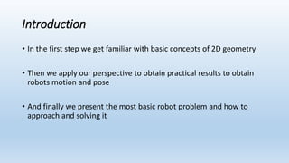
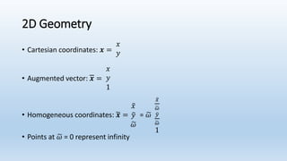
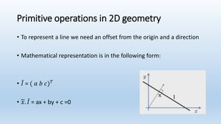
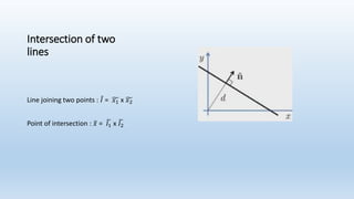
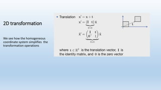
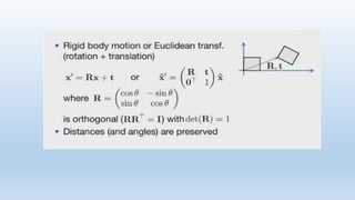
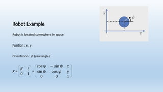
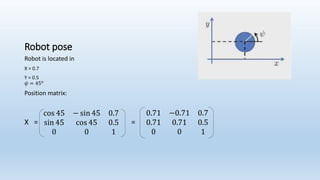
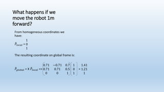
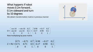
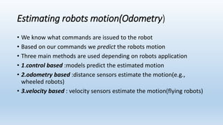
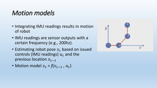
This document discusses robot navigation and pose estimation. It begins with an introduction to basic 2D geometry concepts like Cartesian and homogeneous coordinates. It then covers primitive operations in 2D geometry like representing lines and finding the intersection of two lines. Next, it discusses 2D transformations and provides an example of calculating a robot's pose and how its position would change if it moves forward or rotates. Finally, it discusses estimating a robot's motion through odometry, control-based models, and velocity sensors to integrate its movements over time.

1. Robot Navigation

2. Introduction
• In the first step we get familiar with basic concepts of 2D geometry
• Then we apply our perspective to obtain practical results to obtain
robots motion and pose
• And finally we present the most basic robot problem and how to
approach and solving it

3. 2D Geometry
• Cartesian coordinates: 𝒙 =
𝑥
𝑦
• Augmented vector: 𝒙 =
𝑥
𝑦
1
• Homogeneous coordinates: 𝒙 =
𝑥
𝑦
𝜔
= 𝜔
𝑥
𝜔
𝑦
𝜔
1
• Points at 𝜔 = 0 represent infinity

4. Primitive operations in 2D geometry
• To represent a line we need an offset from the origin and a direction
• Mathematical representation is in the following form:
• 𝐼 = ( 𝑎 𝑏 𝑐) 𝑇
• 𝑥. 𝐼 = ax + by + c =0

5. Intersection of two
lines
Line joining two points : 𝐼 = 𝑥1 x 𝑥2
Point of intersection : 𝑥 = 𝐼1 x 𝐼2

6. 2D transformation
We see how the homogeneous
coordinate system simplifies the
transformation operations

8. Robot Example
Robot is located somewhere in space
Position : x , y
Orientation : 𝜓 (yaw angle)
X =
𝑅 𝑡
0 1
=
cos 𝜓 − sin 𝜓 𝑥
sin 𝜓 cos 𝜓 𝑦
0 0 1

9. Robot pose
Robot is located in
X = 0.7
Y = 0.5
𝜓 = 45 𝜊
Position matrix:
X =
cos 45 − sin 45 0.7
sin 45 cos 45 0.5
0 0 1
=
0.71 −0.71 0.7
0.71 0.71 0.5
0 0 1

10. What happens if we
move the robot 1m
forward?
The resulting coordinate on global frame is:
𝑃𝑔𝑙𝑜𝑏𝑎𝑙 = X 𝑃𝑙𝑜𝑐𝑎𝑙 =>
0.71 −0.71 0.7
0.71 0.71 0.5
0 0 1
1
0
1
=
1.41
1.21
1
From homogeneous coordinates we
have:
𝑃𝑙𝑜𝑐𝑎𝑙 =
1
0
1

11. What happens if robot
moves 0.2m forward ,
0.1m sideward and turn
by 10 degrees
We obtain transformation matrix in previous manner
U =
cos 10 − sin 10 0.2
sin 10 cos 10 0.1
0 0 1
=
0.98 −0.17 0.2
0.17 0.98 0.1
0 0 1
Now multiplying by pose matrix
𝑥 = XU =
0.71 −0.71 0.7
0.71 0.71 0.5
0 0 1
0.98 −0.17 0.2
0.17 0.98 0.1
0 0 1

12. Estimating robots motion(Odometry)
• We know what commands are issued to the robot
• Based on our commands we predict the robots motion
• Three main methods are used depending on robots application
• 1.control based :models predict the estimated motion
• 2.odometry based :distance sensors estimate the motion(e.g.,
wheeled robots)
• 3.velocity based : velocity sensors estimate the motion(flying robots)

13. Motion models
• Integrating IMU readings results in motion
of robot
• IMU readings are sensor outputs with a
certain frequency (e.g., 200hz).
• Estimating robot pose 𝑥 𝑡 based on issued
controls (IMU readings) 𝑢 𝑡 and the
previous location 𝑥 𝑡−1
• Motion model 𝑥 𝑡 = f(𝑥 𝑡−1 , 𝑢 𝑡)