Risk Return.ppt

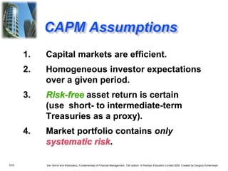
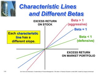
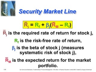
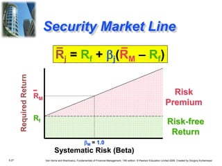
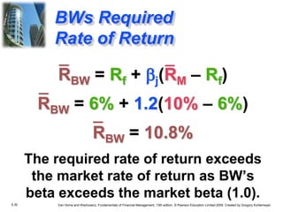
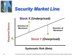
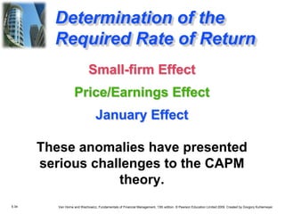
5.1 Van Horne and Wachowicz, Fundamentals of Financial Management, 13th edition. © Pearson Education Limited 2009. Created by Gregory Kuhlemeyer.
Chapter 5
Risk and
Return

Defining Return
Income received on an investment
plus any change in market price,
usually expressed as a percent of
the beginning market price of the
investment.
Dt + (Pt – Pt - 1 )
Pt - 1
R =

Return Example
The stock price for Stock A was $10 per
share 1 year ago. The stock is currently
trading at $9.50 per share and shareholders
just received a $1 dividend. What return
was earned over the past year?

Return Example
The stock price for Stock A was $10 per
share 1 year ago. The stock is currently
trading at $9.50 per share and shareholders
just received a $1 dividend. What return
was earned over the past year?
$1.00 + ($9.50 – $10.00 )
$10.00
R = = 5%

Defining Risk
What rate of return do you expect on your
investment (savings) this year?
What rate will you actually earn?
Does it matter if it is a bank CD or a share
of stock?
The variability of returns from
those that are expected.

Determining Expected
Return (Discrete Dist.)
R = S ( Ri )( Pi )
R is the expected return for the asset,
Ri is the return for the ith possibility,
Pi is the probability of that return
occurring,
n is the total number of possibilities.
n
I = 1

How to Determine the Expected
Return and Standard Deviation
Stock BW
Ri Pi (Ri)(Pi)
-0.15 0.10 –0.015
-0.03 0.20 –0.006
0.09 0.40 0.036
0.21 0.20 0.042
0.33 0.10 0.033
Sum 1.00 0.090
The
expected
return, R,
for Stock
BW is .09
or 9%

Determining Standard
Deviation (Risk Measure)
s = S ( Ri – R )2( Pi )
Standard Deviation, s, is a statistical
measure of the variability of a distribution
around its mean.
It is the square root of variance.
Note, this is for a discrete distribution.
n
i = 1

How to Determine the Expected
Return and Standard Deviation
Stock BW
Ri Pi (Ri)(Pi) (Ri - R )2(Pi)
–0.15 0.10 –0.015 0.00576
–0.03 0.20 –0.006 0.00288
0.09 0.40 0.036 0.00000
0.21 0.20 0.042 0.00288
0.33 0.10 0.033 0.00576
Sum 1.00 0.090 0.01728

Determining Standard
Deviation (Risk Measure)
n
i=1
s = S ( Ri – R )2( Pi )
s = .01728
s = 0.1315 or 13.15%

Coefficient of Variation
The ratio of the standard deviation of
a distribution to the mean of that
distribution.
It is a measure of RELATIVE risk.
CV = s/R
CV of BW = 0.1315 / 0.09 = 1.46

Discrete versus. Continuous
Distributions
0
0.05
0.1
0.15
0.2
0.25
0.3
0.35
0.4
–0.15 –0.03 9% 21% 33%
Discrete Continuous
0
0.005
0.01
0.015
0.02
0.025
0.03
0.035
-50%
-41%
-32%
-23%
-14%
-5%
4%
13%
22%
31%
40%
49%
58%
67%

Certainty Equivalent (CE) is the
amount of cash someone would
require with certainty at a point in
time to make the individual
indifferent between that certain
amount and an amount expected to
be received with risk at the same
point in time.
Risk Attitudes

Certainty equivalent > Expected value
Risk Preference
Certainty equivalent = Expected value
Risk Indifference
Certainty equivalent < Expected value
Risk Aversion
Most individuals are Risk Averse.
Risk Attitudes

You have the choice between (1) a guaranteed
dollar reward or (2) a coin-flip gamble of
$100,000 (50% chance) or $0 (50% chance).
The expected value of the gamble is $50,000.
• Mary requires a guaranteed $25,000, or more, to
call off the gamble.
• Raleigh is just as happy to take $50,000 or take
the risky gamble.
• Shannon requires at least $52,000 to call off the
gamble.
Risk Attitude Example

What are the Risk Attitude tendencies of each?
Risk Attitude Example
Mary shows “risk aversion” because her
“certainty equivalent” < the expected value of
the gamble.
Raleigh exhibits “risk indifference” because her
“certainty equivalent” equals the expected value
of the gamble.
Shannon reveals a “risk preference” because her
“certainty equivalent” > the expected value of
the gamble.

RP = S ( Wj )( Rj )
RP is the expected return for the portfolio,
Wj is the weight (investment proportion)
for the jth asset in the portfolio,
Rj is the expected return of the jth asset,
m is the total number of assets in the
portfolio.
Determining Portfolio
Expected Return
m
J = 1

Combining securities that are not perfectly,
positively correlated reduces risk.
INVESTMENT
RETURN
TIME TIME
TIME
SECURITY E SECURITY F
Combination
E and F
Diversification and the
Correlation Coefficient

Systematic Risk is the variability of return
on stocks or portfolios associated with
changes in return on the market as a whole.
Unsystematic Risk is the variability of return
on stocks or portfolios not explained by
general market movements. It is avoidable
through diversification.
Total Risk = Systematic Risk +
Unsystematic Risk
Total Risk = Systematic
Risk + Unsystematic Risk

Total
Risk
Unsystematic risk
Systematic risk
STD
DEV
OF
PORTFOLIO
RETURN
NUMBER OF SECURITIES IN THE PORTFOLIO
Factors such as changes in the nation’s
economy, tax reform by the Congress,
or a change in the world situation.

Total
Risk
Unsystematic risk
Systematic risk
STD
DEV
OF
PORTFOLIO
RETURN
NUMBER OF SECURITIES IN THE PORTFOLIO
Factors unique to a particular company
or industry. For example, the death of a
key executive or loss of a governmental
defense contract.

CAPM is a model that describes the
relationship between risk and
expected (required) return; in this
model, a security’s expected
(required) return is the risk-free rate
plus a premium based on the
systematic risk of the security.
Capital Asset
Pricing Model (CAPM)

1. Capital markets are efficient.
2. Homogeneous investor expectations
over a given period.
3. Risk-free asset return is certain
(use short- to intermediate-term
Treasuries as a proxy).
4. Market portfolio contains only
systematic risk.
CAPM Assumptions

An index of systematic risk.
It measures the sensitivity of a
stock’s returns to changes in
returns on the market portfolio.
The beta for a portfolio is simply a
weighted average of the individual
stock betas in the portfolio.
What is Beta?

EXCESS RETURN
ON STOCK
EXCESS RETURN
ON MARKET PORTFOLIO
Beta < 1
(defensive)
Beta = 1
Beta > 1
(aggressive)
Each characteristic
line has a
different slope.
Characteristic Lines
and Different Betas

Rj is the required rate of return for stock j,
Rf is the risk-free rate of return,
bj is the beta of stock j (measures
systematic risk of stock j),
RM is the expected return for the market
portfolio.
Rj = Rf + bj(RM – Rf)
Security Market Line

Rj = Rf + bj(RM – Rf)
bM = 1.0
Systematic Risk (Beta)
Rf
RM
Required
Return
Risk
Premium
Risk-free
Return

• Obtaining Betas
• Can use historical data if past best represents the
expectations of the future
• Can also utilize services like Value Line, Ibbotson
Associates, etc.
• Adjusted Beta
• Betas have a tendency to revert to the mean of 1.0
• Can utilize combination of recent beta and mean
• 2.22 (0.7) + 1.00 (0.3) = 1.554 + 0.300 = 1.854 estimate

Lisa Miller at Basket Wonders is attempting
to determine the rate of return required by
their stock investors. Lisa is using a 6% Rf
and a long-term market expected rate of
return of 10%. A stock analyst following the
firm has calculated that the firm beta is 1.2.
What is the required rate of return on the
stock of Basket Wonders?
Determination of the
Required Rate of Return

RBW = Rf + bj(RM – Rf)
RBW = 6% + 1.2(10% – 6%)
RBW = 10.8%
The required rate of return exceeds
the market rate of return as BW’s
beta exceeds the market beta (1.0).
BWs Required
Rate of Return

Lisa Miller at BW is also attempting to
determine the intrinsic value of the stock.
She is using the constant growth model.
Lisa estimates that the dividend next period
will be $0.50 and that BW will grow at a
constant rate of 5.8%. The stock is currently
selling for $15.
What is the intrinsic value of the stock?
Is the stock over or underpriced?
Intrinsic Value of BW

The stock is OVERVALUED as
the market price ($15) exceeds
the intrinsic value ($10).
$0.50
10.8% – 5.8%
Intrinsic
Value
=
= $10
Intrinsic Value of BW

Systematic Risk (Beta)
Rf
Required
Return
Direction of
Movement
Direction of
Movement
Stock Y (Overpriced)
Stock X (Underpriced)

Small-firm Effect
Price/Earnings Effect
January Effect
These anomalies have presented
serious challenges to the CAPM
theory.
Required Rate of Return

Risk Return.ppt

Recommended

Recommended

More Related Content

Similar to Risk Return.ppt

Similar to Risk Return.ppt (20)

Recently uploaded

Recently uploaded (20)

Risk Return.ppt