reinforcement learning

1. Reinforcement Learning in
Recommender Systems
BY GHERGHE IOANA-DELIA, GRIGORE DIANA-N ICOLETA, PINTILIE IOAN A, VULPOIU ALEXANDRU

2. Recommendations with Negative Feedback via Pairwise Deep
Reinforcement Learning
ABSTRACT
In this paper, we propose a novel recommender system with the capability of continuously
improving its strategies during the interactions with users. We model the sequential
interactions between users and a recommender system as a Markov Decision Process (MDP)
and leverage Reinforcement Learning (RL) to automatically learn the optimal strategies via
recommending trial-and-error items and receiving reinforcements of these items from users’
feedback which can be both positive and negative.

3. INTRODUCTION
Efforts have been made on utilizing reinforcement learning for recommender systems. Some
approaches included modeling the recommender system as a MDP process and estimating the
transition probability and then the Q-value table. However, these methods may become inflexible with
the increasing number of items for recommendations. Thus, we leverage Deep Q-Network (DQN), an
(adapted) artificial neural network, as a non-linear approximator to estimate the action-value function
in RL.
When we design recommender systems, positive feedback (clicked /ordered feedback) represents the
users’ preference and thus is the most important information to make recommendations. In reality,
users also skip some recommended items during the recommendation procedure so it is necessary to
incorporate such negative feedback.

4. PROBLEM STATEMENT
The Markov Decision Process (MDP), consists of a tuple of five elements (S, A, P, R, γ ) as follows:
• State space S: A state st S
∈ is defined as the browsing history of a user before time t. The items in st are sorted in
chronological order.
• Action space A: The action at A
∈ of RA is to recommend items to a user at time t. Without the loss of generality, we
assume that the agent only recommends one item to the user each time.
• Reward R: After the RA takes an action at at the state st , i.e., recommending an item to a user, the user browses this
item and provides their feedback. They can skip (not click), click, or order this item, and the RA receives immediate
reward r(st, at ) according to the user’s feedback.
• Transition probability P: Transition probability p(st+1 |st , at ) defines the probability of state transition from st to st+1
when RA takes action at . We assume that the MDP satisfies p(st+1 |st , at , ...,s1, a1) = p(st+1 |st , at ).
• Discount factor γ : γ [0, 1] defines the discount factor when we measure the present value of future reward. In
∈
particular, when γ=0, RA only considers the immediate reward. In other words, when γ=1, all future rewards can be
counted fully into that of the current action.

5. THE PROPOSED DEERS FRAMEWORK
Although the positive items represent the key information about users’ preference, this system will not change its state
or update its strategy when users skip the recommended items. Thus, the state should not only contain positive items
that the user clicked or ordered, but also incorporate negative (skipped) items.
We define state and transition process as follows:
State s: s = (s+ ,s−) S
∈ is a state, where s+ = {i1, · · · ,iN } is defined as the previous N items that a user clicked or ordered
recently, and s− = {j1, · · · , jN } is the previous N items that the user skipped recently. The items in s+ and s− are processed
in chronological order.
Transition from s to s′ : When RA recommends item a at state s = (s+,s−) to a user, if users skip the recommended item,
we keep s′+ = s+ and update s′− = {j2, · · · , jN , a}. If users click or order the recommended item, update s′+ = {i2, · · · ,iN , a},
while keeping s′− = s−. Then set s = (s
′ ′+ ,s′−).

6. Figure 4 illustrates our new DQN architecture. Instead of just concatenating
clicked/ordered/skipped items, we introduce a RNN with Gated Recurrent Units (GRU) to
capture users’ sequential preference.
The inputs of GRU are the embeddings of user’s recently clicked /ordered items {i1, · · · ,iN},
while we use the output (final hidden state hN ) as the representation of the positive state,
i.e., s+ = hN . We obtain negative state s− in a similar way. Here we leverage GRU rather than
Long Short-Term Memory (LSTM) because that GRU outperforms LSTM for capturing users’
sequential behaviors in recommendation tasks.
As shown in Figure 4, we feed positive input (positive signals) and negative input
(negative signals) separately in the input layer. Also, different from traditional fully
connected layers, we separate the first few hidden layers for positive input and
negative input. The intuition behind this architecture is to recommend an item that is
similar to the clicked/ordered items (left part), while dissimilar to the skipped items
(right part).

7. The Pairwise Regularization Term
With deep investigations on the users’ logs, we found that in most
recommendation sessions, the RA recommends some items belonging
to the same category (e.g. telephone), while users click/order a part of
them and skip others. We illustrate a real example of a
recommendation session in Table 1.
At time 2, we name a5 as the competitor item of a2. Sometimes, one item could have multiple “competitor” items; thus
we select the item at the closest time as the “competitor” item.
We select one target item’s competitor item according to three requirements:
1) the “competitor” item belongs to the same category with the target item;
2) user gives different types of feedback to the “competitor” item and the target item;
3) the “competitor” item is at the closest time to the target item.
To maximize the difference of Q-values between target and competitor items, we add a regularization term α to the
equation of the loss function.

8. Off-policy Training Task Offline Test Online Test
We train the proposed model based on users’ offline log, which records the
interaction history between RA’s policy b(st) and users’ feedback. RA takes the action
based on the off-policy b(st) and obtains the feedback from the offline log
(Algorithm 1).
The intuition of our offline test method is that, for a given recommendation session,
the recommender agent reranks the items in this session according to the items’ Q-
value calculated by the trained DQN, and recommends the item with maximal Q-
value to the user (Algorithm 2).
The simulated online environment is also trained on users’ logs, but not on the same data for training the DEERS framework. We test the
simulator on users’ logs and experimental results demonstrate that the simulated online environment has overall 90% precision for
immediate feedback prediction tasks (Algorithm 3).

9. EXPERIMENTS
We evaluate our method on a dataset of September, 2017 from JD.com. We collect 1,000,000 recommendation
sessions (9,136,976 items) in temporal order, and use the first 70% as the training set and the other 30% as test set.
For a given session, the initial state is collected from the previous sessions of the user. In this paper, we leverage N = 10
previously clicked/ordered items as positive state and N = 10 previously skipped items as negative state. The reward r
of skipped/clicked/ordered items are empirically set as 0, 1, and 5, respectively. The dimension of the embedding of
items is 50, and we set the discounted factor γ = 0.95. For the parameters of the proposed framework such as α and γ ,
we select them via cross-validation. Correspondingly, we also do parameter-tuning for baselines for a fair comparison.
We will discuss more details about parameter selection for the proposed framework in the following subsections.
For the architecture of Deep Q-network, we leverage a 5-layer neural network, in which the first 3 layers are
separated for positive and negative signals, and the last 2 layers connect both positive and negative signals, and
outputs the Q-value of a given state and action.
As we consider our offline test task as a reranking task, we select MAP and NDCG@40 as the metrics to evaluate the
performance.

10. Performance Comparison for Offline Test
We compare the proposed framework with the following representative
baseline methods:
CF: Collaborative filtering - making automatic predictions about the interests
of a user by collecting preference information from many users
FM: Factorization Machines combine the advantages of support vector
machines with factorization models.
GRU: This baseline utilizes the Gated Recurrent Units (GRU). To make
comparison fair, it also keeps previous N = 10 clicked/ordered items as states.
DEERS-p: We use a Deep Q-network only with positive feedback
(clicked/ordered items).
The results are shown in Figure 5
To sum up, we can draw answers to two questions:
(1) the proposed framework outperforms representative baselines;
(2) negative feedback can help the recommendation performance.

11. Performance Comparison for Online Test
We do online tests on the aforementioned simulated online environment, and compare DEERS with GRU and several variants of DEERS.
Note that we do not include CF and FM baselines as offline tests since CF and FM are not applicable to the simulated online environment.
GRU: The same GRU as in the above subsection.
DEERS-p: The same DEERS-p as in the above subsection.
DEERS-f: This variant is a traditional 5-layer DQN where all layers are fully connected. Note that the state is also captured by GRU.
DEERS-t: In this variant, we remove GRU units and just concatenate the previous N = 10 clicked/ordered items as positive state and
previous N = 10 skipped items as negative state.
DEERS-r: This variant is to evaluate the performance of the pairwise regularization term, so we set α = 0 to eliminate the pairwise
regularization term.
As the test stage is based on the simulator, we can artificially control the length of recommendation sessions to study the performance in
short and long sessions. We define short sessions with 100 recommended items, while long sessions with 300 recommended items. The
results are shown in Figure 6.
In summary, appropriately redesigning DQN architecture to incorporate negative
feedback, leveraging GRU to capture users’ dynamic preference and introducing
the pairwise regularization term can boost the recommendation performance.

12. Reinforcement learning to rank in e-commerce search engine:
Formalization, analysis, and application
ABSTRACT
Ranking items in a search is a multi-step decision-making problem that usually requires
Learning to Rank (LTR) methods. LTR methods assume that steps in a session are independent,
when in reality they can be highly correlated. In order to use the way in which steps relate to
each other, the paper uses RL to learn an optimal ranking policy that maximizes the expected
accumulative rewards in a search session.

13. INTRODUCTION
Search session between the user and the search engine is a multi-step ranking problem with the following steps
1. user inputs a query in the blank
2. search engine ranks the related items and displays the top K items
3. user makes operations (clicks, buys, requests a new page of the query aka view more)
4. when a new page is requested, the engine reranks the rest of the items and displays top k
All the steps repeat until the user buys items/leaves the search session (usually multiple rounds of this process)
This method
Considers a multi-step sequential ranking problem and proposes a new RL algorithm for learning an optimal ranking policy. The
contributions are:
• definition of search session Markov Decision Process to formulate the problem by identifying the state space, reward function,
state transition function
• proof that maximizing accumulative rewards is necessary → different ranking steps in a session are tightly correlated, rather than
independent
• new algorithm → deterministic policy gradient with full backup estimation → fit for the problem of high reward variance and
unbalanced reward distribution → hardly dealt with even in state of the art RL
• empirical demonstration → algorithm performs much better than online LTR

14. PROBLEM FORMULATION
Search Session Modelling
Top-k list → for an item set, a ranking function and a positive integer k, the top list Lk is an ordered item list which contains
the top K items when applying the ranking function f to the item set D
Item page → for each step t during a session, the item page pt is the top-K list resulted by applying the ranking action at-1 of
the search engine to the set of unranked items in the last decision step t-1. (initially, D0 = D)
Item page history → in a search session, q is the input query. For the initial step, the initial item page history is q. For each
later decision step, the item page history up to h is ht = ht-1 and pt where ht-1 is the page history up to the step t-1 and pt is the
item page of step t
Users may choose to purchase items or just leave at different steps of a session. If we treat all possible users as an
environment which samples user behaviors, this would mean that after observing any item page history, the environment
may terminate a search session with a certain probability of transaction conversion or abandonment.
Conversion probability → for any item page history in a search session ht, B(ht) is the conversion event that a user purchases
an item after observing ht. The conversion probability of ht, which is denoted by b(ht) is the averaged probability that B(ht)
occurs when ht takes place.

15. Abandon probability → for any item page history in a search session, L(ht) is the abandon event that a user leaves the session after
observing ht. l(ht) is the averaged probability that L(ht) occurs when ht takes place
Continuing probability → user continues searching after observing ht.
These 2 types define how the state of the environment will change after at-1 is taken in ht-1:
• terminating the search session by purchasing an item in ht (probability b(ht))
• leaving the search session with probability l(ht)
• continuing the search session from ht with probability 1-b(ht)-l(ht)
Search Session MDP
Agent → search engine
Environment → Population of all possible users
States of the environment → indication of user status in the corresponding item page histories (continuation, abandonment, transaction
conversion)
Action space → depending on the ranking task, can be continuous or discrete
Transition function → directly based on the conversion + abandonment probabilities
Reward function → highly depends on the goal of a task

16. ANALYSIS OF SSMDP
Reward Function
Reward metric in online LTR → user clicks, but in E-commerce scenarios → successful transaction between users and
sellers
This reward function → encourages more successful transactions
• after observing the item page history, a user will purchase an item with a conversion probability and although
different users may choose different items to buy, from a statistical view, the deal prices of the transactions
occurring must follow an underlying distribution
• for a history page, we use m(ht+1) to denote the expected deal price of ht+1
The agent will only receive a positive reward from the environment only when its ranking action leads to a successful
transaction → otherwise, it is 0

17. ALGORITHM - policy gradient algorithm for learning an optimal ranking policy in a search session MDP (SSMDP)
• policy gradient → directly optimizing a parameterized policy function addresses policy representation issue +
large-scale action space issue
• given a SSMDP, and a parameterized policy function, the objective of the agent is to find an optimal parameter for
the said function which maximizes the expectation of the T-step returns along all the possible trajectories
(trajectory = s0, a0, r0, s1, a1, r1, .., sT and trajectory follows a distribution under the policy parameter)
• if we reach a terminal state of the trajectory in less than T steps, the sum of the rewards will be truncated in that
state
• gradient leads to the REINFORCE algorithm and provides a framework which generalizes it
The DPG-FBE algorithm
• we use the deterministic policy gradient algorithm (not stochastic) to learn an optimal ranking policy in an SSMDP
because computing the stochastic policy gradient may require more samples
• difficulty we face → estimating the value function, caused by the high variance (deal price varies over a wide
range) and unbalanced distribution (the conversion events lead by (s, a) occur much less frequently than abandon
and continuation which produce zero rewards) of the immediate rewards in each state (0 or the expected deal
price)

18. • estimating the value function by Monte Carlo evaluation/temporal-difference
learning → inaccurate update of the value function parameters
• solution → similar to the model-based reinforcement learning approaches (they
maintain an approximate model of the environment)
• sampling errors caused by immediate rewards or returns are avoided and the
computational cost of full backups is similar to that of one-step sample backups
(like Q-learning)
• algorithm is based on the deterministic policy gradient theorem and the full
backup estimation of the Q-value functions
• we don’t need to model the entire reward and state transition functions, we only
need to build the conversion probability model, the continuing probability model
and the expected deal price model (can be trained using online/offline data by any
statistical learning method)
• parameters θ and w will be updated after any search session
• exploration (line 3) can be done by ε-greedy or adding random noise to the output
of the parameterized policy function
• we prefer nonlinear methods (neural networks) for learning the policy and value
function due to the large space of an SSMDP → replay buffer + target updates also

19. EXPERIMENTS
• a simulated experiment in which an online shopping simulator is constructed to test DPG-FBE and some other state-of-
the-art LTR algorithms
• a real application in which the algorithm is applied in TaoBao
Simulation
1. Statistical information of items and user behaviours is collected from TaoBao. An item is represented by an n-
dimensional feature vector x and a ranking action of the search engine is a n-dimensional weight vector. The ranking
score of the item is the inner product of the two vectors.
2. 20 important features related to the item category dress (price, quality) are chosen and an item set is generated by
sampling 1000 items from a distribution approximated with all the items of the dress category. Each page contains 10
items so that there are at most 100 ranking rounds in each search session.
3. In a ranking round, the user operations on the current item page (clicks/abandonment/purchase) are simulated by a
user behaviour model.

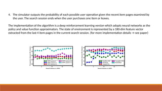
20. 4. The simulator outputs the probability of each possible user operation given the recent item pages examined by
the user. The search session ends when the user purchases one item or leaves.
The implementation of the algorithm is a deep reinforcement learning version which adopts neural networks as the
policy and value function approximators. The state of environment is represented by a 180-dim feature vector
extracted from the last 4 item pages in the current search session. (for more implementation details → see paper)

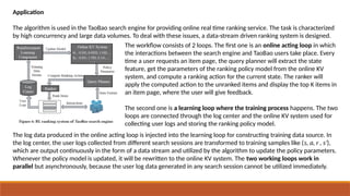
21. Application
The algorithm is used in the TaoBao search engine for providing online real time ranking service. The task is characterized
by high concurrency and large data volumes. To deal with these issues, a data-stream driven ranking system is designed.
The workflow consists of 2 loops. The first one is an online acting loop in which
the interactions between the search engine and TaoBao users take place. Every
time a user requests an item page, the query planner will extract the state
feature, get the parameters of the ranking policy model from the online KV
system, and compute a ranking action for the current state. The ranker will
apply the computed action to the unranked items and display the top K items in
an item page, where the user will give feedback.
The second one is a learning loop where the training process happens. The two
loops are connected through the log center and the online KV system used for
collecting user logs and storing the ranking policy model.
The log data produced in the online acting loop is injected into the learning loop for constructing training data source. In
the log center, the user logs collected from different search sessions are transformed to training samples like (s, a, r , s′),
which are output continuously in the form of a data stream and utilized by the algorithm to update the policy parameters.
Whenever the policy model is updated, it will be rewritten to the online KV system. The two working loops work in
parallel but asynchronously, because the user log data generated in any search session cannot be utilized immediately.

22. A Deep Reinforcement Learning Framework for News Recomm
endation
ABSTRACT
Personalized news recommendation is a tricky problem, due to dynamic news features and user
preferences. There are some news recommendation systems, but they have three major issues:
• they only try to model current reward (e.g.: click through rate);
• very few studies consider to use user feedback, other than click/no click labels (e.g.: how
frequent user returns);
• the existing methods often recommend similar news to users and it causes the users to get bored.
In this presentation, we will study a recommendation framework based on Deep Q-Learning, which
can model future reward. To improve this system, user return pattern will be considered in addition
to click/ no click labels.

23. INTRODUCTION
In this paper, it’s described a Deep Reinforcement Learning
framework, whose purpose is to solve the three challenges
presented before:
• for the first issue, Deep Q-Learning (DQN) framework is
proposed, because it can consider current reward and future
reward simultaneously;
• for the second problem, user returning is considered as
another form of user feedback, by maintaining an activeness
score for each user;
• for the third challenge,
Dueling Bandit Gradient Descent (DBGD) method is used for
exploration, by choosing random item candidates in the
neighborhood of the current recommender and it ensures that
no unrelated items will be recommended.
The next figure describes the recommendation system proposed:

24. PROBLEM DEFINITION
When a user u sends a news request to the recommendation agent G
at time t, given a candidate set I of news, our algorithm is going to
select a list L of top-k appropriate news for this user. The notations used
in this paper are summarized in the next table:
METHOD
To create a strong online personalized news recommendation system, we will study a solution that proposes a DQN-
based Deep Reinforcement Learning framework. We will use a continuous state feature representation of users and
continuous action feature representation of items as the input to a multi-layer Deep Q-Network to predict the
potential reward. Due to the online update of DQN, this model can deal with the dynamic nature of news
recommendation. DQN can also speculate future interaction between user and news. The model will combine user
activeness and click labels as feedback from users.
For recommendation diversity, Dueling Bandit Gradient Descent (DBGD) method will be used.

25. The figure above represents the model used for the news
recommendation system and it contains two stages: offline
and online.
The offline part consists of extracting four kinds of features
from news and users:
• news features
• user features
• user news features
• context features
A multi-layer Deep Q-Network is used to predict the reward (a combination of user-news click label and user activeness)
from these four kinds of features. This network is trained using the offline user-news click logs.
During the online part, the recommendation agent G interacts with users and updates the network in the following way:
1. PUSH
2. FEEDBACK
3. MINOR UPDATE
4. MAJOR UPDATE
5. REPEAT STEPS 1-4.

26. DEEP REINFORCEMENT RECOMMENDATION
As shown in this figure, we feed the four categories of
features into the network. User features and Context
features are used as state features, while User news
features and Context features are used as action
features. On one hand, the reward for taking action a at
a certain state s is closely related to all the features. On
the other hand, the reward that is determined by the
characteristics of the user himself (e.g., whether this
user is active, whether this user has read enough news
today) is more impacted by the status of the user and
the context only. Based on this observation, we divide
the Q-function into value function V(s) and advantage
function A(s, a), where V(s) is only determined by the
state features, and A(s, a) is determined by both the
state features and the action features.

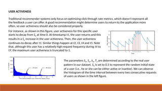
27. USER ACTIVENESS
Traditional recommender systems only focus on optimizing click through rate metrics, which doesn’t represent all
the feedback a user can offer. A good recommendation might determine users to return to the application more
often, so user activeness should also be considered properly.
For instance, as shown in this figure, user activeness for this specific user
starts to decay from S0 at time 0. At timestamp t1, the user returns and this
results in a Sa increase in the user activeness. Then, the user activeness
continues to decay after t1. Similar things happen at t2, t3, t4 and t5. Note
that, although this user has a relatively high request frequency during t4 to
t9, the maximum user activeness is truncated to 1.
The parameters S0, Sa, λ0, T0 are determined according to the real user
pattern in our dataset. S0 is set to 0.5 to represent the random initial state
of a user (i.e., he or she can be either active or inactive). We can observe
the histogram of the time interval between every two consecutive requests
of users as shown in the left figure.

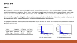
28. EXPERIMENT
DATASET
The experiment is conducted on a sampled offline dataset collected from a commercial news recommendation application and the
system is deployed online to the App for one month. Each recommendation algorithm will give out its recommendation when a news
request arrives and user feedback will be recorded (click or not). In this table, we can see the basic statistics for the sampled data:
In the first offline stage, the training data and testing data are separated by time order (the last two weeks are used as testing data), to
enable the online models to learn the sequential information between different sessions better.
During the second online deploying stage, we use the offline data to pre-train the model, and run all the compared methods in the real
production environment.

29. EVALUATION MEASURES
CTR(click through rate) is calculated as: CTR =
Precision@k is calculated as: Precision@k =
nDCG(normalized discounted cumulative gain): DCG(f) = , where
• r = the rank of items in the recommendation list;
• n = the length of the recommendation list;
• f = the ranking function or algorithm;
• = 1/0, indicates if a click occurs;
• D(r) = the discount, D(r) =
EXPERIMENT SETTING
For this experiment, best parameters are
found using grid search, and their values
are presented in the next table:

30. COMPARED METHODS
 variations of the model described
 the basic model is named DN and it uses a Double Deep Q-Network without future reward;
 when future reward is used, the model is DDQN;
 more components are to DDQN depending on what other algorithms/features are used:
• U = user activeness;
• EG = ε-greedy;
• DBGD = dueling bandit gradient descent;
 baseline algorithms: the models above are compared with the next five baseline methods, which will
conduct online update during the testing stage:
 LR(logistic regression)
 FM(factorization machines)
 W&D(wide and deep)
 LinUCB(linear upper confidence bound)
 HLinUCB(hidden linear upper confidence bound)
For all compared algorithms, the recommendation list is generated by selecting the items with top-k estimated
potential reward (for LinUCB, HLinUCB and our methods) or probability of click (for LR, FM and W&D) of each item.

31. OFFLINE EVALUATION
In this stage, our models are compared with other baselines on the offline
dataset. The offline dataset is static, so only certain pairs of user-news interaction
have been recorded. We can’t observe the change of user activeness and the
exploration strategy can’t explore well due to the limited candidate news set, so
the efficiency of these methods isn’t visible in this situation.
accuracy
• as expected, the models proposed outperform the baseline algorithms;
• the accuracy is even better when future reward is added;
• the results can be observed in the table;
model converge process
• in order to study the convergence process, we will analyze the cumulative CTR
of different methods in the graph on the right;
• the offline data are ordered by time and simulate the process that users send
news request as time goes by;
• all the compared methods will update their models every 100 request
sessions;

32. ONLINE EVALUATION
In the online evaluation stage, we deployed our models and compared algorithms
on a commercial news recommendation application. Users are divided evenly to
different algorithms. In online stage, we can’t only measure the accuracy of
recommendation, but also observe the recommendation diversity for different
algorithms.
accuracy
• different algorithms are compared in terms of CTR, Precision@5 and nDCG;
• the results are similar to those from offline stage, because the solutions
proposed in this article are better and the future reward considerations
represents an improvement;
recommendation diversity
• in order to evaluate the effectiveness of exploration, we calculate the
recommendation diversity of different algorithms using ILS
• the diversity for the news clicked by users is represented in the right table;
• smaller ILS indicates better diversity;
• similarity between news is measured by the cosine similarity between the
bag-of-words vectors of news;

33. Deep reinforcement learning for list-wise recommendations
ABSTRACT
The paper proposes a new recommender system with a more dynamic approach than the one used in
traditional systems. The sequential interactions between the user and the system are modelled as a
Markov Decision Process (MDP) and Reinforcement Learning (RL) is used by recommending trial-and-error
items and leveraging the users’ feedback. An online user-agent interacting environment simulator is used
to pre-train and evaluate the model offline. Moreover, the proposed framework LIRD develops a novel
approach to incorporating list-wise recommendations.
INTRODUCTION
List-wise recommendations are more desired in practice since they allow the systems to provide diverse
and complementary options to their users.
Existing approaches for list-wise recommendations do not take into account the relationship between the
list items - for example, a news feed recommendation system might recommend a list of extremely similar
news articles, when, in reality, a user might be more interested in being provided with diverse topics. The
paper aims to enhance performance by capturing the relationship between the recommended items.

34. Architecture Selection
Generally, there exist two Deep Q-learning architectures, shown in Fig.1 (a)(b). The use of both poses issues when it comes to
recommender systems, and the architecture shown in Fig.1(c) seeks to mitigate them.
• Fig.1(a) depicts the architecture adopted by traditional deep Q-learning. It is suitable for the scenario with high state space and
small action space, but not for the large and dynamic action space scenario.
• Fig.1(b) depicts the second Q-learning architecture. Unlike the previous one, it is suitable for large action space, as it does not
need to store each Q-value in memory. However, it does compute Q-values for all potential actions, which brings in the challenge
of temporal complexity.
• Fig.1(c) depicts the architecture upon which this paper’s recommending policy builds on. The Actor inputs the current state and
aims to output the parameters of a state-specific scoring function. Then the RA (recommender agent) scores all items and selects
an item with the highest score. Next, the Critic uses an approximation architecture to learn a value function (Q-value), which is a
judgement of whether the selected action matches the current state. Finally, according to the judgement from the Critic, the
Actor updates its policy parameters in a direction of recommending performance improvement.
This architecture is both suitable for large action space and reduces redundant computations.

35. Online Environment Simulator
In order to tackle the challenging nature of training and evaluating the framework offline, the paper proposes an
online environment simulator, which inputs current state and a selected action and outputs a simulated online
reward. This enables the framework to train the parameters offline based on the simulated reward. More
specifically, the simulator is built using users’ historical records - it is assumed that, no matter what algorithms a
recommender system adopts, the user feedback to an item will remain unchanged.
Problem Statement
An RA interacts with the environment (or users) by sequentially choosing recommendation items over a sequence
of time steps, so as to maximise its cumulative reward. We model the problem of listwise item recommendation
as Markov Decision Process (MDP), which formally consists of a tuple of five elements (S, A, P, R,γ ).
• State space S. A state st = {st
1
, · · · , st
N
} S
∈ represents the browsing history of a user, i.e. the previous N items
that a user browsed before time t. The items are sorted in chronological order.
• Action space A. An action at = {at
1
, · · · , at
K
} A
∈ is to recommend a list of items to a user at time t based on
current state st , where K is the number of items the RA recommends to user each time.
• Reward R. The RA takes an action at at the state st (= recommends a list of items to a user). The user can then
skip, click, or order these items. Based on this feedback, the RA receives an immediate reward r(st, at).
• P and γ have the usual MDP meanings

36. Instead of extra item information, in this paper, we use the user-agent interaction information, i.e., users’ browsing
history. We treat each item as a word and the clicked items in one recommendation session as a sentence. Then, we
can obtain dense and low-dimensional vector representations for items via word embedding.
The Actor Framework
Current practical recommender systems rely on a scoring or rating system averaged across all users, but this leads to poor
results when there is high variation in users’ interests. To tackle this problem, a state-specific scoring function, which
rates items according to the user's current state, is introduced.
In this section, we define the state s by taking into consideration only positive items, e.g. the previous 10 clicked/ordered
items. This is more efficient than considering the entire browsing history, as a good recommender system should focus on
user preferences.
The Critic Framework
The Critic is designed to leverage an approximator to learn an action-value function Q(st , at), which is a judgement of
whether the action generated by the Actor matches the current state st. Then, according to Q(st , at), the Actor updates its
parameters in a direction of improving performance.

37. The Training Procedure
In order to train the parameters of the proposed framework, DDPG (Deep Deterministic Policy Gradient - a model-free off-
policy algorithm for learning continuous actions) is used.
In each iteration, we have the:
• Transition generating stage: the RA recommends a list of items, observes the reward from the simulator, updates the
state and stores the transition
• Parameter updating stage: the RA samples mini-batches of transitions and the, following DDPG, updates the Actor’s
and the Critic’s parameters.
The Testing Procedure
The testing procedure follows the same algorithm as the training procedure, meaning that the parameters continuously
update while testing.
However, to make comparison between sessions possible, the parameters are set back to the well-trained ones Θµ
and Θπ
after each recommendation session.

38. EXPERIMENTS
Experiments to evaluate the effectiveness of the proposed framework are conducted using a dataset from a real
e-commerce site. The main focus points are: comparison to representative baselines, and analysis of how the
list-wise strategy contributes to performance.
Experimental Settings
• 100,000 recommendation sessions (1,156,675 items) in temporal order were collected, the first 70% were
used as the training set, and the remaining 30% as the testing set
• The positive state is N = 10 previously clicked/ordered items.
• Each time, the RA recommends a list of k = 4 items to users.
• The reward r is set as 0, 1, or 5, corresponding to skipped/clicked/ordered, respectively
• γ = 0.75, dimension of item embedding = 50
• Parameter tuning for baselines is performed.

39. Performance Comparison for Item Recommendations
The proposed framework is compared to the following representative baseline methods:
• CF (Collaborative filtering): a method that makes predictions about the interests of a user by collecting preference
information from many users
• FM (Factorization machines): combines the advantages of support vector machines with factorization models in order
to model higher order interactions
• DNN with backpropagation technique: trained to output the next recommended item, given the embeddings of users’
clicked/ordered items as input
• RNN: also trained to predict what a user will buy next, based on previously clicked/ordered items
• DQN: shares the same architecture as the Critic in the proposed framework
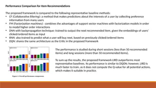
The performance is studied during short sessions (less than 50 recommended
items) and long sessions (more than 50 recommended items).
To sum up the results, the proposed framework LIRD outperforms most
representative baselines. Its performance is similar to DQON; however, LIRD is
much faster to train, as it does not compute the Q-value for all potential actions,
which makes it suitable in practice.

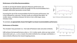
40. Performance of List-Wise Recommendations
In order to see how the listwise approach influences performance, we
investigate how LIRD performs when the length K of the recommendation list is
changed, while other parameters remain fixed.
Increasing the size of the recommendation list first increases performance, but
is then followed by a decrease. The best results are achieved when K=4 - for
smaller values, correlations between list items is lost, while larger values
introduce noise.
To conclude, an appropriately chosen list length K can boost recommendation performance.
Performance of Simulator
The simulator’s key parameter is α - the trade-off between state and action similarity.
LIRD achieves the best performance when α = 0.2. In other words, when we map current
state-action pair pt (st , at ) to a reward, the action-similarity has a stronger contribution, while
state-similarity influences the reward mapping process.