The Bairstow method and Muller method are techniques for calculating the roots of polynomials.
The Bairstow method uses synthetic division to iteratively calculate the roots of a polynomial by dividing it by quadratic factors (x^2 - rx - s) until the remainder is zero. It obtains better approximations of r and s at each iteration to isolate the roots.
The Muller method fits a parabola through three initial guesses to obtain the coefficients a, b, c of the quadratic formula. It then uses the quadratic formula to find the root, and iterates with new guesses to converge on more accurate roots.
Both methods use iterative techniques to gradually converge on the real and complex roots of polynomials without
Los triángulos tienen diferentes clases y propiedades. Una propiedad clave es que la suma de los ángulos interiores de cualquier triángulo siempre es igual a 180 grados.
Syntide Medi-Chem Technology (China) Limited (SMCT) is a chemical synthesis service provider and supplier that offers custom synthesis, contract research and development, process development, and chemical sourcing services to life sciences industries. SMCT specializes in the synthesis of complex molecules, with a focus on chiral compounds, and has the capability to scale syntheses from milligrams to kilograms. SMCT aims to accelerate scientific discovery through cost-effective chemistry solutions and reliable, high-quality service.
The Bairstow method and Muller method are techniques for calculating the roots of polynomials.
The Bairstow method uses synthetic division to iteratively calculate the roots of a polynomial by dividing it by quadratic factors (x^2 - rx - s) until the remainder is zero. It obtains better approximations of r and s at each iteration to isolate the roots.
The Muller method fits a parabola through three initial guesses to obtain coefficients a, b, c. It then uses the quadratic formula on the parabola to find the root, and iterates with new guesses until converging on a solution.
Both methods use iterative techniques to refine initial guesses and isolate the roots of polynomials without using
The Bairstow method is an iterative technique for finding the roots of polynomials by calculating the coefficients of a quadratic factor. It works by taking an initial approximation of the quadratic factor and generating better approximations using partial derivatives until the remainder of dividing the polynomial by the quadratic factor is zero, giving the roots. The method calculates the partial derivatives to update the approximations in a way that avoids having to perform calculations with complex numbers directly. When applied repeatedly, it can find all roots of polynomials of third order or higher.
This document defines and explains different types of matrices:
- Upper and lower triangular matrices have zeros above or below the main diagonal of a square matrix.
- The determinant of a matrix is a scalar value obtained from the products of the matrix's elements according to certain constraints.
- A banded matrix is a sparse matrix with nonzero elements confined to a diagonal band around the main diagonal.
- The transpose of a matrix exchanges the rows and columns of the original matrix.
- For matrix multiplication to be defined, the number of columns of the left matrix must equal the number of rows of the right matrix.
This document defines and describes different types of matrices including:
- Upper and lower triangular matrices
- Determinants which are scalars obtained from products of matrix elements according to constraints
- Band matrices which are sparse matrices with nonzero elements confined to diagonals
- Transpose matrices which exchange the rows and columns of a matrix
- Inverse matrices which when multiplied by the original matrix produce the identity matrix
Este documento explica los conceptos básicos de los polígonos. Define un polígono como una figura geométrica formada por tres o más segmentos de línea que se intersectan pero permanecen en el mismo plano. Detalla los elementos de un polígono como lados, vértices y ángulos. Explica propiedades como que un polígono de n lados tiene n vértices y ángulos interiores, y cómo calcular el número de diagonales y la suma de los ángulos interiores y exteriores. Finalmente, incluye algunos ejercicios
Gaussian Elimination is a variation of the Gauss elimination method that can solve up to 15-20 simultaneous equations with 8-10 significant digits of precision on a computer. It differs from Gaussian elimination by normalizing all rows when using them as the pivot equation, resulting in an identity matrix rather than a triangular matrix. This avoids needing to perform back substitution. The method is demonstrated through solving a system of 3 equations with 3 unknowns via Gaussian elimination, resulting in values for the 3 unknowns. Advantages of the Gaussian-Jordan method include requiring approximately 50% fewer operations than Gaussian elimination and providing a direct method for obtaining the inverse matrix.
Tratatimiento numerico de ecuaciones diferenciales (2)daferro
1) El documento describe métodos para resolver ecuaciones elípticas y parabólicas, incluyendo la ecuación de Laplace y la ecuación de conducción de calor.
2) Se explica el método de Crank-Nicholson para resolver numéricamente la ecuación de conducción de calor de manera implícita.
3) También se cubren métodos como el de Liebmann para resolver ecuaciones elípticas de manera iterativa.
Este documento describe métodos numéricos para resolver ecuaciones diferenciales ordinarias, incluidos los métodos de Euler, punto medio, Heun y Runge-Kutta. Explica cómo cada método estima la pendiente para predecir valores futuros y mejorar la precisión de la solución. También proporciona ejemplos numéricos para ilustrar la aplicación de los métodos.
Este documento presenta métodos numéricos para aproximar la solución de ecuaciones diferenciales parciales (EDP) de segundo orden. Explica el método de diferencias finitas para discretizar EDP y aproximar derivadas. Luego, cubre métodos explícitos para resolver ecuaciones parabólicas de conducción de calor mediante diferencias temporales y espaciales, analizando su convergencia, estabilidad y tratamiento de condiciones de frontera. Finalmente, presenta un ejemplo numérico de aplicación del método explícito
Este documento describe métodos iterativos para resolver sistemas de ecuaciones lineales, como el método de Jacobi y el método de Gauss-Seidel. Explica que los métodos iterativos calculan sucesivas aproximaciones a la solución de forma recurrente hasta converger, a diferencia de los métodos directos que obtienen la solución exacta. También discute conceptos como matriz diagonalmente dominante y cuando es más conveniente usar métodos iterativos frente a métodos directos.
El documento describe métodos iterativos para resolver sistemas de ecuaciones lineales, como el método de Jacobi y Gauss-Seidel. El método de Jacobi involucra iterar una ecuación de recurrencia para mejorar sucesivamente las aproximaciones a la solución, mientras que Gauss-Seidel mejora sobre Jacobi actualizando las variables una por una en cada iteración en lugar de todas juntas.
Este documento presenta la factorización LU de una matriz como el producto de una matriz triangular inferior y una superior. Explica el proceso de descomposición de una matriz A en las matrices L y U, y cómo usar esta descomposición para resolver sistemas de ecuaciones lineales de la forma Ax=b de manera más eficiente que otros métodos. Incluye ejemplos numéricos para ilustrar los pasos de la factorización LU y su aplicación para resolver sistemas de ecuaciones.
Este documento describe la factorización LU de una matriz. Explica que la factorización LU descompone una matriz A en el producto de una matriz triangular inferior L y una matriz triangular superior U. Esto permite resolver sistemas de ecuaciones lineales de forma más eficiente mediante sustitución hacia adelante y hacia atrás. Incluye ejemplos numéricos para ilustrar cómo aplicar la factorización LU para resolver sistemas de ecuaciones.
La factorización LU descompone una matriz A en el producto de una matriz triangular inferior L y una matriz triangular superior U. Esto permite resolver sistemas de ecuaciones lineales de forma más eficiente mediante sustitución hacia adelante y hacia atrás. El documento explica el proceso de obtener las matrices L y U y usarlas para resolver un sistema de ecuaciones dado como ejemplo.
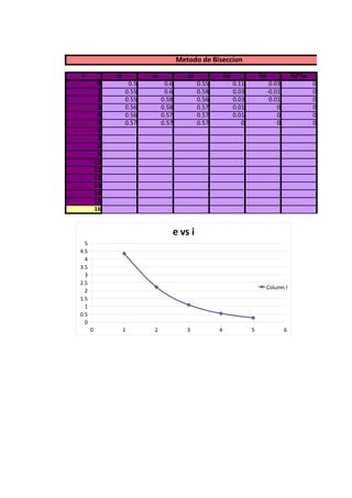
This document describes the bisection method for finding the root of a function. It shows an example of applying the bisection method to find a root between 0.5 and 0.6 over 15 iterations. At each iteration, it calculates the function values at the lower and upper bounds and their product to determine if a sign change has occurred, identifying a root within the bounds. The root converges to 0.57 and the error decreases with each iteration.
Este documento describe la factorización LU de una matriz. Explica que la factorización LU descompone una matriz A en el producto de una matriz triangular inferior L y una matriz triangular superior U. Esto permite resolver sistemas de ecuaciones lineales de forma más eficiente mediante sustitución hacia adelante y hacia atrás. El documento también incluye ejemplos numéricos para ilustrar los pasos del proceso de factorización LU.
The Bairstow method and Muller method are techniques for calculating the roots of polynomials.
The Bairstow method uses synthetic division to iteratively calculate the roots of a polynomial by dividing it by quadratic factors (x^2 - rx - s) until the remainder is zero. It obtains better approximations of r and s at each iteration to isolate the roots.
The Muller method fits a parabola through three initial guesses to obtain coefficients a, b, c. It then uses the quadratic formula on the parabola to find the root, and iterates with new guesses until converging on a solution.
Both methods use iterative techniques to refine initial guesses and isolate the roots of polynomials without using
The Bairstow method is an iterative technique for finding the roots of polynomials by calculating the coefficients of a quadratic factor. It works by taking an initial approximation of the quadratic factor and generating better approximations using partial derivatives until the remainder of dividing the polynomial by the quadratic factor is zero, giving the roots. The method calculates the partial derivatives to update the approximations in a way that avoids having to perform calculations with complex numbers directly. When applied repeatedly, it can find all roots of polynomials of third order or higher.
This document defines and explains different types of matrices:
- Upper and lower triangular matrices have zeros above or below the main diagonal of a square matrix.
- The determinant of a matrix is a scalar value obtained from the products of the matrix's elements according to certain constraints.
- A banded matrix is a sparse matrix with nonzero elements confined to a diagonal band around the main diagonal.
- The transpose of a matrix exchanges the rows and columns of the original matrix.
- For matrix multiplication to be defined, the number of columns of the left matrix must equal the number of rows of the right matrix.
This document defines and describes different types of matrices including:
- Upper and lower triangular matrices
- Determinants which are scalars obtained from products of matrix elements according to constraints
- Band matrices which are sparse matrices with nonzero elements confined to diagonals
- Transpose matrices which exchange the rows and columns of a matrix
- Inverse matrices which when multiplied by the original matrix produce the identity matrix
This document defines and describes different types of matrices including:
- Upper and lower triangular matrices
- Determinants which are scalars obtained from products of matrix elements according to constraints
- Band matrices which are sparse matrices with nonzero elements confined to diagonals
- Transpose matrices which exchange the rows and columns of a matrix
- Inverse matrices which when multiplied by the original matrix produce the identity matrix
Este documento explica los conceptos básicos de los polígonos. Define un polígono como una figura geométrica formada por tres o más segmentos de línea que se intersectan pero permanecen en el mismo plano. Detalla los elementos de un polígono como lados, vértices y ángulos. Explica propiedades como que un polígono de n lados tiene n vértices y ángulos interiores, y cómo calcular el número de diagonales y la suma de los ángulos interiores y exteriores. Finalmente, incluye algunos ejercicios
Gaussian Elimination is a variation of the Gauss elimination method that can solve up to 15-20 simultaneous equations with 8-10 significant digits of precision on a computer. It differs from Gaussian elimination by normalizing all rows when using them as the pivot equation, resulting in an identity matrix rather than a triangular matrix. This avoids needing to perform back substitution. The method is demonstrated through solving a system of 3 equations with 3 unknowns via Gaussian elimination, resulting in values for the 3 unknowns. Advantages of the Gaussian-Jordan method include requiring approximately 50% fewer operations than Gaussian elimination and providing a direct method for obtaining the inverse matrix.
Tratatimiento numerico de ecuaciones diferenciales (2)daferro
1) El documento describe métodos para resolver ecuaciones elípticas y parabólicas, incluyendo la ecuación de Laplace y la ecuación de conducción de calor.
2) Se explica el método de Crank-Nicholson para resolver numéricamente la ecuación de conducción de calor de manera implícita.
3) También se cubren métodos como el de Liebmann para resolver ecuaciones elípticas de manera iterativa.
Este documento describe métodos numéricos para resolver ecuaciones diferenciales ordinarias, incluidos los métodos de Euler, punto medio, Heun y Runge-Kutta. Explica cómo cada método estima la pendiente para predecir valores futuros y mejorar la precisión de la solución. También proporciona ejemplos numéricos para ilustrar la aplicación de los métodos.
Este documento presenta métodos numéricos para aproximar la solución de ecuaciones diferenciales parciales (EDP) de segundo orden. Explica el método de diferencias finitas para discretizar EDP y aproximar derivadas. Luego, cubre métodos explícitos para resolver ecuaciones parabólicas de conducción de calor mediante diferencias temporales y espaciales, analizando su convergencia, estabilidad y tratamiento de condiciones de frontera. Finalmente, presenta un ejemplo numérico de aplicación del método explícito
Este documento describe métodos iterativos para resolver sistemas de ecuaciones lineales, como el método de Jacobi y el método de Gauss-Seidel. Explica que los métodos iterativos calculan sucesivas aproximaciones a la solución de forma recurrente hasta converger, a diferencia de los métodos directos que obtienen la solución exacta. También discute conceptos como matriz diagonalmente dominante y cuando es más conveniente usar métodos iterativos frente a métodos directos.
El documento describe métodos iterativos para resolver sistemas de ecuaciones lineales, como el método de Jacobi y Gauss-Seidel. El método de Jacobi involucra iterar una ecuación de recurrencia para mejorar sucesivamente las aproximaciones a la solución, mientras que Gauss-Seidel mejora sobre Jacobi actualizando las variables una por una en cada iteración en lugar de todas juntas.
Este documento presenta la factorización LU de una matriz como el producto de una matriz triangular inferior y una superior. Explica el proceso de descomposición de una matriz A en las matrices L y U, y cómo usar esta descomposición para resolver sistemas de ecuaciones lineales de la forma Ax=b de manera más eficiente que otros métodos. Incluye ejemplos numéricos para ilustrar los pasos de la factorización LU y su aplicación para resolver sistemas de ecuaciones.
Este documento describe la factorización LU de una matriz. Explica que la factorización LU descompone una matriz A en el producto de una matriz triangular inferior L y una matriz triangular superior U. Esto permite resolver sistemas de ecuaciones lineales de forma más eficiente mediante sustitución hacia adelante y hacia atrás. Incluye ejemplos numéricos para ilustrar cómo aplicar la factorización LU para resolver sistemas de ecuaciones.
La factorización LU descompone una matriz A en el producto de una matriz triangular inferior L y una matriz triangular superior U. Esto permite resolver sistemas de ecuaciones lineales de forma más eficiente mediante sustitución hacia adelante y hacia atrás. El documento explica el proceso de obtener las matrices L y U y usarlas para resolver un sistema de ecuaciones dado como ejemplo.
This document describes the bisection method for finding the root of a function. It shows an example of applying the bisection method to find a root between 0.5 and 0.6 over 15 iterations. At each iteration, it calculates the function values at the lower and upper bounds and their product to determine if a sign change has occurred, identifying a root within the bounds. The root converges to 0.57 and the error decreases with each iteration.
Este documento describe la factorización LU de una matriz. Explica que la factorización LU descompone una matriz A en el producto de una matriz triangular inferior L y una matriz triangular superior U. Esto permite resolver sistemas de ecuaciones lineales de forma más eficiente mediante sustitución hacia adelante y hacia atrás. El documento también incluye ejemplos numéricos para ilustrar los pasos del proceso de factorización LU.