Pytorch A DetailedOverview Agladze Mikhail
download
https://ebookbell.com/product/pytorch-a-detailed-overview-
agladze-mikhail-58304306
Explore and download more ebooks at ebookbell.com
2.
Here are somerecommended products that we believe you will be
interested in. You can click the link to download.
Deep Learning With Pytorch A Practical Approach To Building Neural
Network Models Using Pytorch Vishnu Subramanian
https://ebookbell.com/product/deep-learning-with-pytorch-a-practical-
approach-to-building-neural-network-models-using-pytorch-vishnu-
subramanian-49155920
Deep Learning With Pytorch A Practical Approach To Building Neural
Network Models Using Pytorch Subramanian
https://ebookbell.com/product/deep-learning-with-pytorch-a-practical-
approach-to-building-neural-network-models-using-pytorch-
subramanian-20640420
Modern Computer Vision With Pytorch A Practical And Comprehensive
Guide To Understanding Deep Learning And Multimodal Models For
Realworld Vision Tasks 2nd Edition V Kishore Ayyadevarayeshwanth Reddy
https://ebookbell.com/product/modern-computer-vision-with-pytorch-a-
practical-and-comprehensive-guide-to-understanding-deep-learning-and-
multimodal-models-for-realworld-vision-tasks-2nd-edition-v-kishore-
ayyadevarayeshwanth-reddy-57684292
Pytorch Recipes A Problemsolution Approach To Build Train And Deploy
Neural Network Models 2nd Edition 2nd Pradeepta Mishra
https://ebookbell.com/product/pytorch-recipes-a-problemsolution-
approach-to-build-train-and-deploy-neural-network-models-2nd-
edition-2nd-pradeepta-mishra-47374278
3.
Pytorch Recipes AProblemsolution Approach 1st Edition Pradeepta
Mishra
https://ebookbell.com/product/pytorch-recipes-a-problemsolution-
approach-1st-edition-pradeepta-mishra-7359328
Deep Learning Examples With Pytorch And Fastai A Developers Cookbook
Bernhard J Mayr
https://ebookbell.com/product/deep-learning-examples-with-pytorch-and-
fastai-a-developers-cookbook-bernhard-j-mayr-43818478
Deep Learning With Pytorch Stepbystep A Beginners Guide Daniel Voigt
Godoy
https://ebookbell.com/product/deep-learning-with-pytorch-stepbystep-a-
beginners-guide-daniel-voigt-godoy-37598380
Deep Learning With Pytorch Stepbystep A Beginners Guide Daniel Voigt
Godoy
https://ebookbell.com/product/deep-learning-with-pytorch-stepbystep-a-
beginners-guide-daniel-voigt-godoy-46856630
A Greater Foundation For Machine Learning Engineering The Hallmarks Of
The Great Beyond In Pytorch R Tensorflow And Python 1st Edition Dr
Ganapathi Pulipaka
https://ebookbell.com/product/a-greater-foundation-for-machine-
learning-engineering-the-hallmarks-of-the-great-beyond-in-pytorch-r-
tensorflow-and-python-1st-edition-dr-ganapathi-pulipaka-36378294
6.
Contents
Disclaimer
Introduction To PyTorch:A Deep Learning Framework
Overview of PyTorch and Its Ecosystem
Building Neural Networks with PyTorch
PyTorch Autograd: Automatic Differentiation
Understanding and Using PyTorch Datasets and DataLoaders
Training and Evaluating Models in PyTorch
Setting Up Your PyTorch Environment
Installing PyTorch on Different Platforms
Setting Up Virtual Environments for PyTorch Projects
Configuring CUDA for GPU Acceleration
Using Conda for PyTorch Dependency Management
Integrating PyTorch with Jupyter Notebooks
Verifying Your PyTorch Installation
Managing PyTorch Versions and Upgrades
Tensors: The Core Data Structure Of PyTorch
Introduction to Tensors in PyTorch
Tensor Creation Methods and Initialization
Tensor Manipulation Techniques
Broadcasting in PyTorch Tensors
Advanced Tensor Indexing and Slicing
Tensor Operations and Computations
Handling Tensor Shapes and Dimensions
7.
Building Your FirstNeural Network With PyTorch
Introduction to Neural Networks
Defining Neural Network Layers in PyTorch
Forward and Backward Propagation Mechanisms
Loss Functions and Optimization Algorithms
Implementing Activation Functions
Saving and Loading PyTorch Models
Visualizing Training Progress with TensorBoard
Deep Dive Into Autograd And Computational Graphs
Understanding Computational Graphs in PyTorch
Automatic Differentiation Mechanics
Building and Visualizing Computational Graphs
Gradient Descent and Backpropagation
Custom Autograd Functions
Handling Dynamic Computational Graphs
Optimizing Performance with Autograd
Optimizers And Loss Functions: Training Your Model
Introduction to Optimization in PyTorch
Commonly Used Optimizers: SGD, Adam, and Beyond
Customizing and Implementing Your Own Optimizers
Loss Functions: Concepts and Selection Criteria
Implementing and Comparing Different Loss Functions
Advanced Techniques: Learning Rate Schedulers and Warm
Restarts
Practical Tips for Debugging and Improving Training Performance
8.
Data Loading AndProcessing With PyTorch Datasets And
DataLoaders
Introduction to PyTorch Datasets and DataLoaders
Creating Custom Datasets in PyTorch
Data Transformations and Augmentations
Efficient Data Loading with DataLoader
Handling Imbalanced Datasets in PyTorch
Parallel Data Loading with PyTorch
Debugging Data Loading Issues
Convolutional Neural Networks (CNNs) In PyTorch
Introduction to Convolutional Neural Networks
Building a Simple CNN from Scratch in PyTorch
Understanding Convolution and Pooling Layers
Implementing Various CNN Architectures: LeNet, AlexNet, and VGG
Transfer Learning with Pre-trained CNNs in PyTorch
Advanced CNN Techniques: Batch Normalization and Dropout
Visualizing CNN Filters and Feature Maps
Recurrent Neural Networks (RNNs) And LSTMs In PyTorch
Introduction to Recurrent Neural Networks (RNNs)
Implementing Basic RNNs in PyTorch
Understanding Long Short-Term Memory (LSTM) Networks
Building LSTM Networks in PyTorch
Training and Evaluating RNN and LSTM Models
Advanced RNN Techniques: Bidirectional RNNs and GRUs
Applications of RNNs and LSTMs in Natural Language Processing
Transfer Learning And Fine-Tuning With PyTorch
9.
Fundamentals of TransferLearning
Leveraging Pre-trained Models for New Tasks
Techniques for Fine-Tuning Neural Networks
Practical Applications of Transfer Learning
Evaluating Transfer Learning Performance
Advanced Strategies for Model Adaptation
Case Studies and Real-World Examples
Natural Language Processing (NLP) With PyTorch
Introduction to Natural Language Processing with PyTorch
Tokenization and Text Preprocessing Techniques
Building Word Embeddings from Scratch
Implementing Sequence-to-Sequence Models
Attention Mechanisms and Transformer Models
Deploying NLP Models in Production
Evaluating and Improving NLP Model Performance
Generative Adversarial Networks (GANs) In PyTorch
Introduction to Generative Adversarial Networks (GANs)
Implementing GANs from Scratch in PyTorch
Training GANs: Techniques and Best Practices
Conditional GANs and Their Applications
Advanced GAN Architectures: DCGAN, CycleGAN, and StyleGAN
Evaluating GAN Performance: Metrics and Methods
Practical Applications of GANs in Various Domains
Graph Neural Networks (GNNs) In PyTorch
Introduction to Graph Neural Networks (GNNs)
10.
Graph Data Structuresand Representations in PyTorch
Implementing Graph Convolutional Networks (GCNs) in PyTorch
Training and Evaluating GNN Models
Advanced GNN Architectures: Graph Attention Networks (GATs)
and Beyond
Practical Applications of GNNs in Real-World Scenarios
Optimizing GNN Performance and Scalability
Hyperparameter Tuning And Model Optimization
Understanding Hyperparameters and Their Impact on Model
Performance
Strategies for Hyperparameter Tuning: Grid Search, Random
Search, and Beyond
Using Bayesian Optimization for Hyperparameter Tuning in PyTorch
Automating Hyperparameter Tuning with Libraries like Optuna and
Ray Tune
Techniques for Model Optimization: Pruning, Quantization, and
Distillation
Leveraging AutoML for Efficient Model Optimization
Best Practices for Monitoring and Logging During Hyperparameter
Tuning
Deploying PyTorch Models In Production
Preparing PyTorch Models for Production Deployment
Deploying PyTorch Models with Flask and FastAPI
Serving PyTorch Models with TorchServe
Integrating PyTorch Models with Docker Containers
Monitoring and Managing PyTorch Models in Production
11.
Scaling PyTorch ModelInference with Kubernetes
Security Considerations for Deploying PyTorch Models
PyTorch In The Cloud: Leveraging Cloud Services
Leveraging Cloud Storage for PyTorch Data Management
Using Cloud-Based GPUs and TPUs for PyTorch Training
Automating PyTorch Workflows with Cloud Pipelines
Serverless Computing for PyTorch Inference
Scaling PyTorch Applications with Cloud Load Balancers
Integrating PyTorch with Cloud-Based Machine Learning Services
Cost Optimization Strategies for Running PyTorch on Cloud
Debugging And Profiling PyTorch Models
Introduction to Debugging Techniques in PyTorch
Utilizing PyTorch Debugger (pdb) for Model Inspection
Identifying and Resolving Common Errors in PyTorch Models
Profiling PyTorch Code for Performance Optimization
Using PyTorch Profiler for Detailed Performance Analysis
Memory Management and Debugging in PyTorch
Best Practices for Efficient Debugging and Profiling
Advanced Custom Layers And Modules
Creating Custom Layers with PyTorch
Building Modular and Reusable Components
Implementing Parametric and Non-Parametric Layers
Advanced Techniques for Layer Initialization
Incorporating Custom Loss Functions
Designing and Utilizing Custom Activation Functions
12.
Integrating Custom Layerswith Pre-built Models
Model Interpretability And Explainability In PyTorch
Understanding Model Interpretability: Concepts and Importance
Techniques for Visualizing Model Predictions
Using SHAP Values for Interpretability in PyTorch
Implementing LIME for Local Model Explanations
Interpreting Convolutional Models with Grad-CAM
Exploring Feature Importance in PyTorch Models
Best Practices for Enhancing Model Explainability
Using PyTorch For Reinforcement Learning
Fundamentals of Reinforcement Learning with PyTorch
Implementing Q-Learning Algorithms in PyTorch
Deep Q-Networks (DQN) and Enhancements
Policy Gradient Methods and Applications
Actor-Critic Algorithms: Theory and Practice
Multi-Agent Reinforcement Learning with PyTorch
Real-World Case Studies and Applications of PyTorch in
Reinforcement Learning
Distributed Training With PyTorch
Fundamentals of Distributed Training
Implementing Data Parallelism in PyTorch
Model Parallelism Strategies
Distributed Data-Parallel Training with PyTorch
Optimizing Communication in Distributed Training
Fault Tolerance and Checkpointing in Distributed Systems
Scalable Hyperparameter Tuning in Distributed Environments
13.
Integrating PyTorch WithOther Libraries And Tools
Integrating PyTorch with Scikit-Learn for Machine Learning
Pipelines
Using PyTorch with Pandas for Data Manipulation and Analysis
Combining PyTorch with NumPy for Efficient Numerical
Computations
Enhancing Visualization with PyTorch and Matplotlib
Leveraging PyTorch with OpenCV for Computer Vision Tasks
Integrating PyTorch with Hugging Face Transformers for NLP
Using PyTorch with Dask for Scalable Data Processing
PyTorch Lightning: Simplifying Training And Experimentation
Introduction to PyTorch Lightning: Streamlining Deep Learning
Setting Up PyTorch Lightning for Your Projects
Building Modular Models with PyTorch Lightning
Simplifying Training Loops with PyTorch Lightning Trainer
Configuring Callbacks and Loggers in PyTorch Lightning
Handling Multi-GPU and TPU Training in PyTorch Lightning
Best Practices for Experimentation and Reproducibility with PyTorch
Lightning
Best Practices For PyTorch Code And Model Management
Organizing PyTorch Projects: Directory Structure and Naming
Conventions
Implementing Modular and Reusable PyTorch Code
Version Control and Collaboration with Git for PyTorch Projects
Effective Documentation Practices for PyTorch Code
Ensuring Code Quality with Linters and Static Analysis Tools
14.
Testing PyTorch Models:Unit Tests and Integration Tests
Automating Workflows with Continuous Integration/Continuous
Deployment (CI/CD) for PyTorch
Case Studies: Real-World Applications Of PyTorch
Utilizing PyTorch for Real-Time Object Detection
Implementing PyTorch in Autonomous Vehicle Navigation
PyTorch in Healthcare: Predictive Analytics and Diagnostics
Financial Market Predictions Using PyTorch Models
Enhancing E-commerce Recommendations with PyTorch
PyTorch for Natural Language Understanding in Customer Support
Deploying PyTorch for Climate Modeling and Weather Forecasting
Future Trends And Developments In PyTorch
Exploring PyTorch for Synthetic Data Generation and Simulation
Emerging Techniques in Model Compression and Acceleration
PyTorch in Edge Computing: Strategies and Applications
Integrating PyTorch with Quantum Computing
Advancements in PyTorch for Federated Learning
PyTorch and Automated Machine Learning (AutoML) Innovations
Future Directions in PyTorch for Ethical AI and Fairness
Resources And Community: Getting Help And Staying Updated
Navigating the PyTorch Documentation
Engaging with the PyTorch Forums and Discussion Boards
Leveraging Social Media for PyTorch Updates and Networking
Participating in PyTorch Meetups and Conferences
Contributing to PyTorch Open Source Projects
Utilizing Online Courses and Tutorials for PyTorch Mastery
Disclaimer
The information providedin this content is for educational and/or
general informational purposes only. It is not intended to be a
substitute for professional advice or guidance. Any reliance you place
on this information is strictly at your own risk. We make no
representations or warranties of any kind, express or implied, about
the completeness, accuracy, reliability, suitability or availability with
respect to the content for any purpose. Any action you take based
on the information in this content is strictly at your own discretion.
We are not liable for any losses or damages in connection with the
use of this content. Always seek the advice of a qualified
professional for any questions you may have regarding a specific
topic.
18.
Introduction To PyTorch:A
Deep Learning Framework
Overview of PyTorch and Its Ecosystem
PyTorch stands as one of the leading frameworks in the deep
learning landscape, renowned for its dynamic computational graph
and ease of use. Developed by Facebook's AI Research lab, PyTorch
has rapidly gained popularity among researchers and practitioners
alike. This section aims to provide a comprehensive overview of
PyTorch and its ecosystem, highlighting its core components,
features, and the broader infrastructure that supports its application
in various domains.
At its core, PyTorch is a Python-based library designed for deep
learning. It offers a flexible and intuitive interface that allows
developers to build and train neural networks efficiently. One of the
key strengths of PyTorch is its dynamic computation graph, which
enables users to modify the graph on-the-fly during runtime. This
feature contrasts with static computation graphs used by other
frameworks, providing greater flexibility and ease of debugging. As a
result, PyTorch is particularly favored in research settings where
rapid prototyping and experimentation are essential.
PyTorch's tensor library is foundational to its functionality. Tensors,
which are multidimensional arrays, serve as the primary data
structure in PyTorch. They support a wide range of mathematical
operations and can be easily transferred between the CPU and GPU,
facilitating efficient computation. The library also includes automatic
differentiation, a feature that simplifies the process of computing
gradients for optimization algorithms. This capability is crucial for
training neural networks, as it automates the backpropagation
process, allowing for seamless gradient computation.
19.
Beyond its corefunctionalities, PyTorch boasts a rich ecosystem of
tools and libraries that extend its capabilities. One of the most
notable is TorchVision, a library specifically tailored for computer
vision tasks. TorchVision provides pre-trained models, image
datasets, and a suite of transformation functions, streamlining the
development of vision-based applications. For natural language
processing (NLP), the TorchText library offers similar utilities,
including text preprocessing tools and pre-trained word embeddings.
In addition to these domain-specific libraries, PyTorch has integrated
support for distributed training through its TorchElastic and
TorchDistributed libraries. These tools enable efficient training of
large-scale models across multiple GPUs and nodes, making PyTorch
suitable for both research and production environments.
Furthermore, PyTorch Lightning, a high-level interface built on top of
PyTorch, abstracts much of the boilerplate code associated with
training routines, promoting cleaner and more maintainable
codebases.
The PyTorch ecosystem also includes a wealth of community-
contributed resources. The PyTorch Hub, for instance, serves as a
repository for pre-trained models contributed by the community.
Users can easily integrate these models into their projects,
leveraging state-of-the-art architectures without the need for
extensive training. Additionally, the PyTorch community forum and
various online platforms provide a collaborative space for users to
share knowledge, troubleshoot issues, and stay updated with the
latest advancements.
Another significant component of the PyTorch ecosystem is its
integration with other machine learning frameworks and tools.
PyTorch seamlessly interoperates with libraries such as NumPy,
SciPy, and scikit-learn, allowing users to leverage a broad range of
scientific computing tools. Moreover, PyTorch's compatibility with the
ONNX (Open Neural Network Exchange) format enables the export
and import of models across different frameworks, facilitating model
deployment in diverse environments.
20.
The versatility ofPyTorch extends to its support for various
deployment options. TorchServe, an open-source model serving
framework, simplifies the process of deploying PyTorch models in
production. It provides functionalities such as multi-model serving,
model versioning, and metrics logging, ensuring robust and scalable
deployment workflows. Additionally, PyTorch Mobile enables
developers to run PyTorch models on mobile devices, expanding the
reach of AI applications to edge devices.
In summary, PyTorch's dynamic computation graph, intuitive
interface, and comprehensive ecosystem make it a powerful tool for
deep learning. Its core components, including the tensor library and
automatic differentiation, provide a solid foundation for building and
training neural networks. The ecosystem, enriched by domain-
specific libraries, distributed training support, and community
contributions, further enhances its applicability across various fields.
By integrating seamlessly with other tools and offering versatile
deployment options, PyTorch empowers developers to create,
experiment, and deploy AI solutions with ease.
21.
Building Neural Networkswith PyTorch
Neural networks, inspired by the human brain, are the cornerstone
of modern artificial intelligence and machine learning. They consist
of layers of interconnected nodes, or neurons, that process and
learn from data. PyTorch, with its intuitive design and dynamic
nature, provides an excellent platform for constructing and training
these networks. In this section, we will explore the process of
building neural networks using PyTorch, from defining model
architectures to training and evaluating them.
To begin, let's discuss the fundamental components of a neural
network. At its core, a neural network comprises an input layer, one
or more hidden layers, and an output layer. Each layer contains a
certain number of neurons, and the connections between these
neurons are characterized by weights that are adjusted during
training. The primary objective of training a neural network is to
optimize these weights to minimize the error between the predicted
and actual outputs.
In PyTorch, the `torch.nn` module provides a comprehensive suite
of tools for constructing neural networks. The most common way to
define a neural network is by creating a subclass of
`torch.nn.Module` and implementing the `__init__` and `forward`
methods. The `__init__` method initializes the layers of the
network, while the `forward` method defines the forward pass,
which is the process of computing the output from the input data.
Consider the following example of a simple feedforward neural
network, also known as a multilayer perceptron (MLP). This network
consists of an input layer, two hidden layers, and an output layer:
import torch
import torch.nn as nn
import torch.optim as optim
class SimpleNN(nn.Module):
def __init__(self, input_size, hidden_size, output_size):
22.
super(SimpleNN, self).__init__()
self.fc1 =nn.Linear(input_size, hidden_size)
self.fc2 = nn.Linear(hidden_size, hidden_size)
self.fc3 = nn.Linear(hidden_size, output_size)
def forward(self, x):
x = torch.relu(self.fc1(x))
x = torch.relu(self.fc2(x))
x = self.fc3(x)
return x
In this example, `SimpleNN` is a subclass of `torch.nn.Module`.
The `__init__` method initializes three fully connected (linear)
layers, and the `forward` method defines the forward pass, applying
the ReLU activation function to the outputs of the first two layers.
The final layer produces the output without an activation function,
which is suitable for regression tasks. For classification tasks, a
softmax activation or similar function would typically be applied to
the output layer.
Once the network architecture is defined, the next step is to train
the network. Training involves feeding input data through the
network, computing the loss, and updating the weights using an
optimization algorithm. PyTorch simplifies this process with its
`torch.optim` module, which provides various optimization
algorithms, such as stochastic gradient descent (SGD) and Adam.
Consider the following example of training the `SimpleNN` model on
a hypothetical dataset:
# Define the model, loss function, and optimizer
model = SimpleNN(input_size=10, hidden_size=20, output_size=1)
criterion = nn.MSELoss()
optimizer = optim.SGD(model.parameters(), lr=0.01)
# Training loop
for epoch in range(100):
for inputs, targets in dataloader:
23.
# Zero thegradients
optimizer.zero_grad()
# Forward pass
outputs = model(inputs)
loss = criterion(outputs, targets)
# Backward pass and optimization
loss.backward()
optimizer.step()
print(f'Epoch [{epoch+1}/100], Loss: {loss.item()}')
In this example, we first define the model, loss function, and
optimizer. The `nn.MSELoss` function computes the mean squared
error loss, which is suitable for regression tasks. The `optim.SGD`
optimizer updates the model's parameters using stochastic gradient
descent with a learning rate of 0.01. The training loop iterates over
the dataset for a specified number of epochs, performing the
forward pass, computing the loss, performing the backward pass,
and updating the weights in each iteration.
Evaluating the performance of a trained neural network is crucial for
understanding its effectiveness. This typically involves measuring the
model's accuracy on a separate validation or test dataset. PyTorch
provides tools for computing various metrics, such as accuracy,
precision, and recall. Consider the following example of evaluating
the `SimpleNN` model:
# Evaluation mode
model.eval()
# Disable gradient computation
with torch.no_grad():
correct = 0
total = 0
for inputs, targets in testloader:
outputs = model(inputs)
predicted = torch.argmax(outputs, dim=1)
24.
total += targets.size(0)
correct+= (predicted == targets).sum().item()
accuracy = correct / total
print(f'Accuracy: {accuracy * 100:.2f}%')
In this example, we set the model to evaluation mode using
`model.eval()` and disable gradient computation with
`torch.no_grad()` to improve efficiency. We then iterate over the
test dataset, compute the model's predictions, and calculate the
accuracy by comparing the predicted and actual labels.
In addition to feedforward neural networks, PyTorch supports
various other types of neural networks, such as convolutional neural
networks (CNNs) and recurrent neural networks (RNNs). CNNs are
widely used for image processing tasks, while RNNs are suitable for
sequential data, such as time series or natural language.
Consider the following example of a simple CNN for image
classification:
class SimpleCNN(nn.Module):
def __init__(self):
super(SimpleCNN, self).__init__()
self.conv1 = nn.Conv2d(in_channels=1, out_channels=16,
kernel_size=3, stride=1, padding=1)
self.pool = nn.MaxPool2d(kernel_size=2, stride=2, padding=0)
self.fc1 = nn.Linear(16 * 14 * 14, 10)
def forward(self, x):
x = self.pool(torch.relu(self.conv1(x)))
x = x.view(-1, 16 * 14 * 14)
x = self.fc1(x)
return x
In this example, `SimpleCNN` is a subclass of `torch.nn.Module`.
The `__init__` method initializes a convolutional layer, a max-
pooling layer, and a fully connected layer. The `forward` method
25.
defines the forwardpass, applying the ReLU activation and max-
pooling to the output of the convolutional layer, flattening the tensor,
and passing it through the fully connected layer.
Training and evaluating a CNN follows the same principles as for a
feedforward network, with the primary difference being the use of
image datasets and data augmentation techniques to improve
generalization.
In conclusion, building neural networks with PyTorch involves
defining the model architecture, training the model, and evaluating
its performance. PyTorch's `torch.nn` and `torch.optim` modules
provide a comprehensive set of tools for constructing and optimizing
neural networks, while its flexible and dynamic nature allows for
rapid experimentation and prototyping. By mastering these
techniques, you can harness the full potential of PyTorch to develop
and deploy powerful deep learning models.
26.
PyTorch Autograd: AutomaticDifferentiation
Understanding the fundamental concepts of automatic differentiation
is crucial for anyone delving into deep learning using PyTorch.
Autograd, PyTorch's automatic differentiation library, facilitates the
computation of gradients, which are essential for optimizing neural
networks. This section provides a comprehensive exploration of
PyTorch's Autograd, elucidating its features, capabilities, and
practical applications in deep learning.
At its core, Autograd records operations performed on tensors to
create a computational graph, enabling the calculation of gradients
through backpropagation. This dynamic approach allows for the
seamless computation of derivatives, making it an indispensable tool
for training neural networks.
To begin, consider a simple example of creating tensors and
performing basic operations. When a tensor's attribute
`requires_grad` is set to `True`, PyTorch tracks all operations on
that tensor, constructing a computational graph. This graph is then
used to compute gradients during the backward pass. For instance,
let's examine the following example:
import torch
# Create tensors
x = torch.tensor(2.0, requires_grad=True)
y = torch.tensor(3.0, requires_grad=True)
# Perform operations
z = x * y + y
# Compute gradients
z.backward()
# Print gradients
print(x.grad) # Output: 3.0
print(y.grad) # Output: 2.0
27.
In this example,the tensors `x` and `y` have `requires_grad` set
to `True`, indicating that Autograd should track their operations.
The expression `z = x * y + y` creates a computational graph with
`z` as the output. When `z.backward()` is called, PyTorch computes
the gradients of `z` with respect to `x` and `y`, storing them in
`x.grad` and `y.grad`, respectively.
One of the remarkable features of Autograd is its ability to handle
complex operations and functions. For instance, if we define a
custom function and apply it to tensors, Autograd will still be able to
compute the gradients accurately. Consider the following example:
import torch
# Define a custom function
def custom_function(x):
return x 2 + 3 * x + 5
# Create a tensor
x = torch.tensor(1.0, requires_grad=True)
# Apply the custom function
y = custom_function(x)
# Compute the gradient
y.backward()
# Print the gradient
print(x.grad) # Output: 5.0
In this case, the custom function `custom_function` is applied to
the tensor `x`, and Autograd automatically constructs the
computational graph. The gradient of `y` with respect to `x` is then
computed using the `backward()` method.
Autograd also supports higher-order derivatives, which are essential
for certain advanced optimization techniques. To compute higher-
order derivatives, the `grad` method can be used inside the
backward pass. For example:
28.
import torch
# Createa tensor
x = torch.tensor(2.0, requires_grad=True)
# Define a function
y = x 3
# Compute the first derivative
y.backward(create_graph=True)
first_derivative = x.grad
# Compute the second derivative
first_derivative.backward()
second_derivative = x.grad
# Print the derivatives
print(first_derivative) # Output: 12.0
print(second_derivative) # Output: 6.0
Here, the `create_graph` parameter in the `backward()` method is
set to `True`, enabling the construction of a computational graph for
the first derivative. This allows for the computation of higher-order
derivatives by performing additional backward passes.
In practical deep learning applications, Autograd is extensively used
for training neural networks. During training, the loss function's
gradients with respect to the model parameters are computed, and
these gradients are used to update the parameters via optimization
algorithms. Consider the following example of training a simple
linear regression model:
import torch
import torch.nn as nn
import torch.optim as optim
# Define a simple linear regression model
class LinearRegressionModel(nn.Module):
def __init__(self):
29.
super(LinearRegressionModel, self).__init__()
self.linear =nn.Linear(1, 1)
def forward(self, x):
return self.linear(x)
# Create a dataset
x_train = torch.tensor([[1.0], [2.0], [3.0]], requires_grad=True)
y_train = torch.tensor([[2.0], [4.0], [6.0]], requires_grad=True)
# Instantiate the model, loss function, and optimizer
model = LinearRegressionModel()
criterion = nn.MSELoss()
optimizer = optim.SGD(model.parameters(), lr=0.01)
# Training loop
for epoch in range(100):
# Zero the gradients
optimizer.zero_grad()
# Forward pass
outputs = model(x_train)
loss = criterion(outputs, y_train)
# Backward pass
loss.backward()
# Update the weights
optimizer.step()
# Print the final loss
print(loss.item())
In this example, the `LinearRegressionModel` is defined as a
subclass of `nn.Module`, and the training loop involves computing
the loss, performing the backward pass to calculate gradients, and
updating the model parameters using the optimizer. Autograd
automatically tracks the operations and computes the necessary
gradients during the backward pass.
30.
Another powerful featureof Autograd is its ability to handle non-
scalar outputs. In such cases, the `backward()` method requires an
additional argument to specify the gradient of the output with
respect to itself. For instance:
import torch
# Create a tensor
x = torch.tensor([[1.0, 2.0], [3.0, 4.0]], requires_grad=True)
# Define a function
y = x 2
# Compute the gradient
gradient = torch.ones_like(y)
y.backward(gradient)
# Print the gradient
print(x.grad)
Here, the tensor `y` has a non-scalar output, and the `backward()`
method is called with a gradient tensor of ones, enabling the
computation of gradients for each element in `x`.
To sum up, PyTorch's Autograd is a powerful and flexible library for
automatic differentiation, playing a pivotal role in the training of
neural networks. By dynamically constructing computational graphs
and efficiently computing gradients, Autograd simplifies the
optimization process and enables the development of complex deep
learning models. Mastering Autograd is essential for anyone looking
to harness the full potential of PyTorch in their deep learning
endeavors.
31.
Understanding and UsingPyTorch Datasets
and DataLoaders
In deep learning, the preparation and handling of data are
paramount. PyTorch, a versatile and powerful deep learning
framework, provides robust tools to streamline this process through
its `torch.utils.data` module. This section will delve into the
intricacies of PyTorch Datasets and DataLoaders, elucidating their
roles, functionalities, and practical applications in deep learning
workflows.
To commence, let's explore the concept of a Dataset in PyTorch. A
Dataset is an abstract class representing a collection of data samples
and their corresponding labels. It serves as the foundation for data
handling in PyTorch, providing a standardized way to load and
preprocess data. By subclassing `torch.utils.data.Dataset`, users can
create custom datasets tailored to their specific needs.
Consider the following example of a custom Dataset class for a
hypothetical image classification task. This class loads images and
their labels from a directory, applies transformations, and returns the
processed data samples.
import os
from PIL import Image
import torch
from torch.utils.data import Dataset
from torchvision import transforms
class CustomImageDataset(Dataset):
def __init__(self, image_dir, transform=None):
self.image_dir = image_dir
self.transform = transform
self.image_paths = [os.path.join(image_dir, img) for img in
os.listdir(image_dir)]
32.
def __len__(self):
return len(self.image_paths)
def__getitem__(self, idx):
image_path = self.image_paths[idx]
image = Image.open(image_path)
if self.transform:
image = self.transform(image)
label = self._get_label_from_path(image_path)
return image, label
def _get_label_from_path(self, path):
# Placeholder function to extract label from the file path
return 0
In this example, the `CustomImageDataset` class is initialized with
the directory containing images and an optional transformation. The
`__len__` method returns the number of samples in the dataset,
while the `__getitem__` method retrieves an image and its label
based on the provided index. The `_get_label_from_path` function
is a placeholder for extracting labels from the file paths, which can
be customized as needed.
Transformations play a crucial role in preparing data for neural
network training. PyTorch's `torchvision.transforms` module offers a
variety of transformations, such as resizing, normalization, and data
augmentation. These transformations can be composed using
`transforms.Compose` and passed to the Dataset class. For
instance, the following code snippet demonstrates how to apply a
series of transformations to the images in the custom dataset.
transform = transforms.Compose([
transforms.Resize((128, 128)),
transforms.ToTensor(),
transforms.Normalize(mean=[0.5, 0.5, 0.5], std=[0.5, 0.5, 0.5])
])
33.
dataset = CustomImageDataset(image_dir='path/to/images',
transform=transform)
Inthis example, the images are resized to 128x128 pixels, converted
to tensors, and normalized with a mean and standard deviation of
0.5 for each channel. These transformations ensure that the data is
in the appropriate format and range for the neural network.
Moving on, DataLoaders are indispensable for efficient data loading
and batching. A DataLoader wraps a Dataset and provides an
iterable over the data samples, handling batching, shuffling, and
parallel data loading. This is particularly beneficial for large datasets,
where loading the entire dataset into memory is impractical.
The following code snippet illustrates how to create a DataLoader for
the custom image dataset.
from torch.utils.data import DataLoader
dataloader = DataLoader(dataset, batch_size=32, shuffle=True,
num_workers=4)
In this example, the DataLoader is configured to load data in
batches of 32, shuffle the samples at each epoch, and use four
worker processes for parallel data loading. The `batch_size`
parameter determines the number of samples per batch, while
`shuffle` ensures that the data is randomly shuffled at each epoch,
promoting better generalization during training. The `num_workers`
parameter specifies the number of subprocesses to use for data
loading, which can significantly speed up the data loading process.
DataLoaders provide an efficient way to iterate over the dataset
during training. The following code snippet demonstrates a typical
training loop using a DataLoader.
for epoch in range(num_epochs):
for images, labels in dataloader:
# Forward pass
34.
outputs = model(images)
loss= criterion(outputs, labels)
# Backward pass and optimization
optimizer.zero_grad()
loss.backward()
optimizer.step()
print(f'Epoch [{epoch+1}/{num_epochs}], Loss: {loss.item()}')
In this example, the DataLoader iterates over the dataset, returning
batches of images and labels. The model performs a forward pass to
compute the outputs, and the loss is calculated using a predefined
criterion. The gradients are then computed via the backward pass,
and the optimizer updates the model parameters. This process is
repeated for the specified number of epochs, with the loss printed
after each epoch.
Furthermore, PyTorch supports built-in datasets for popular
benchmarks, such as CIFAR-10, MNIST, and ImageNet, through the
`torchvision.datasets` module. These datasets can be easily loaded
and used with DataLoaders, facilitating quick experimentation and
prototyping. For instance, the following code snippet demonstrates
how to load the CIFAR-10 dataset and create a DataLoader.
from torchvision.datasets import CIFAR10
cifar10_dataset = CIFAR10(root='path/to/data', train=True,
transform=transform, download=True)
cifar10_dataloader = DataLoader(cifar10_dataset, batch_size=32,
shuffle=True, num_workers=4)
In this example, the CIFAR-10 dataset is downloaded and
transformed using the specified transformations. A DataLoader is
then created to iterate over the dataset in batches.
In addition to standard datasets, PyTorch provides utilities for
handling data from various sources, such as text, audio, and video.
The `torchtext`, `torchaudio`, and `torchvision` libraries offer
35.
specialized datasets andtransformations for these data types,
enabling seamless integration with PyTorch models.
To summarize, PyTorch Datasets and DataLoaders are essential
components for efficient data handling in deep learning. By providing
a standardized way to load, preprocess, and iterate over data, they
streamline the training process and enable the development of
robust and scalable models. Whether working with custom datasets
or leveraging built-in datasets, mastering these tools is crucial for
any deep learning practitioner.
36.
Training and EvaluatingModels in PyTorch
In the ever-evolving landscape of machine learning, effectively
training and evaluating models is a pivotal process that determines
the success of any deep learning project. PyTorch, a prominent
framework in this domain, offers a plethora of tools and
functionalities to streamline these operations. This section delves
into the intricacies of training and evaluating models using PyTorch,
ensuring that readers gain a comprehensive understanding of these
critical stages.
The journey of training a model commences with the selection of an
appropriate architecture. PyTorch provides a flexible platform for
defining a wide variety of models, from simple linear regressors to
complex convolutional and recurrent networks. Once the model
architecture is defined, the next step is to prepare the data. Data
preparation involves loading the dataset, applying necessary
transformations, and organizing it into batches for efficient
processing.
To illustrate this process, consider a scenario where we aim to train
a deep learning model for image classification. The dataset,
consisting of labeled images, is first loaded and preprocessed.
PyTorch’s `torchvision` library offers a convenient way to handle
image data, providing built-in datasets and transformation utilities.
After the data is ready, it is time to define the model architecture.
For instance, a convolutional neural network (CNN) might be chosen
for its effectiveness in image-related tasks.
With the model architecture and data in place, the next crucial step
is to define the loss function and the optimizer. The loss function
quantifies the difference between the model’s predictions and the
actual labels, guiding the optimization process. PyTorch’s `torch.nn`
module includes a variety of loss functions tailored for different
tasks, such as cross-entropy loss for classification and mean squared
error for regression. The optimizer, on the other hand, is responsible
for updating the model’s parameters to minimize the loss. PyTorch’s
37.
`torch.optim` module offersseveral optimization algorithms,
including stochastic gradient descent (SGD) and Adam, each with its
own advantages and use cases.
The training process involves iterating over the dataset multiple
times, known as epochs. In each epoch, the model processes
batches of data, computes the loss, and updates its parameters. This
iterative process gradually improves the model’s performance.
During training, it is essential to monitor the loss and other relevant
metrics to ensure that the model is learning effectively. Visualizing
these metrics using tools like TensorBoard can provide valuable
insights and help in diagnosing potential issues.
Consider a practical example where we train a CNN on a dataset of
handwritten digits. The dataset is divided into training and validation
sets, with the former used for training the model and the latter for
evaluating its performance. The model is trained for a specified
number of epochs, and the loss and accuracy are tracked throughout
the process. After each epoch, the model’s performance on the
validation set is assessed to ensure it is generalizing well to unseen
data.
Once the training phase is complete, the model’s performance must
be thoroughly evaluated. Evaluation involves testing the model on a
separate test set that was not used during training or validation. This
step provides an unbiased assessment of the model’s generalization
capabilities. Key metrics such as accuracy, precision, recall, and F1-
score are computed to gauge the model’s effectiveness. PyTorch’s
`torchmetrics` library offers a comprehensive suite of metrics for
various tasks, simplifying the evaluation process.
It is worth noting that model evaluation is not a one-time process.
As new data becomes available or the problem requirements evolve,
the model may need to be retrained and re-evaluated. Continuous
monitoring and periodic retraining ensure that the model remains
accurate and relevant over time.
38.
In addition totraditional evaluation metrics, visual inspection of the
model’s predictions can provide valuable insights. For instance, in
image classification tasks, visualizing the predicted and actual labels
for a subset of images can help identify patterns and potential areas
for improvement. Similarly, in natural language processing tasks,
examining the model’s output for sample inputs can reveal strengths
and weaknesses.
Another critical aspect of model evaluation is understanding and
addressing overfitting and underfitting. Overfitting occurs when the
model performs exceptionally well on the training data but fails to
generalize to new data. This can be mitigated through techniques
such as regularization, dropout, and data augmentation.
Underfitting, on the other hand, happens when the model is too
simplistic to capture the underlying patterns in the data. Increasing
the model’s complexity or providing more training data can help
alleviate underfitting.
Hyperparameter tuning is another essential component of training
and evaluating models. Hyperparameters, unlike model parameters,
are set before the training process and significantly influence the
model’s performance. Examples include the learning rate, batch size,
and the number of layers in the network. Tuning these
hyperparameters involves experimenting with different values and
selecting the combination that yields the best performance. PyTorch
integrates well with hyperparameter optimization libraries such as
Optuna, facilitating efficient and automated tuning.
Model interpretability and explainability are gaining prominence in
the field of deep learning. Understanding how a model makes
decisions is crucial, especially in applications where transparency and
trust are paramount. Techniques such as feature importance
analysis, SHAP values, and LIME can shed light on the inner
workings of the model, helping stakeholders understand and trust its
predictions.
Finally, deploying the trained model for inference is the culmination
of the training and evaluation process. PyTorch provides tools for
39.
exporting models tovarious formats, such as ONNX, enabling
deployment across different platforms and environments. Efficient
inference requires optimizing the model for speed and memory
usage, often through techniques like model quantization and
pruning.
To summarize, training and evaluating models in PyTorch is a
multifaceted process that encompasses data preparation, model
definition, loss and optimization, iterative training, and thorough
evaluation. By leveraging PyTorch’s robust ecosystem and adhering
to best practices, practitioners can develop and deploy high-
performing deep learning models that drive impactful outcomes. This
section has provided a detailed exploration of these stages,
equipping readers with the knowledge and tools to excel in their
deep learning endeavors.
40.
Setting Up YourPyTorch
Environment
Installing PyTorch on Different Platforms
Setting up PyTorch on your system can be straightforward if you
follow the appropriate steps for your specific operating system. This
section will provide detailed instructions for installing PyTorch on
Windows, macOS, and Linux. Each platform has its own set of
requirements and installation methods, which will be covered
comprehensively to ensure a smooth setup process.
Windows Installation
To begin with Windows, the first step is to ensure that you have
Python installed on your system. Python can be downloaded from
the official Python website. It is recommended to download the
latest version of Python to ensure compatibility with PyTorch. Once
Python is installed, you can proceed to install PyTorch.
Open your Command Prompt and verify your Python installation by
typing:
python --version
Next, you will need to install pip, the package installer for Python.
Pip is often included with Python installations, but if it is not, you can
install it manually. To check if pip is installed, type:
pip --version
If pip is not installed, download the get-pip.py script from the official
pip website and run it using Python:
python get-pip.py
41.
With pip ready,you can now install PyTorch. The recommended way
to install PyTorch is via the official PyTorch website, where you can
find a command generator that provides the appropriate installation
command based on your system configuration. For a typical
installation, you might use the following command:
pip install torch torchvision torchaudio
This command installs PyTorch along with the torchvision and
torchaudio libraries, which are often used in conjunction with
PyTorch. Once the installation is complete, you can verify it by
starting a Python interpreter and importing PyTorch:
python
import torch
print(torch.__version__)
macOS Installation
For macOS users, the process is similar but with a few platform-
specific considerations. Start by ensuring that you have Homebrew
installed. Homebrew is a package manager for macOS that simplifies
the installation of software. Open your Terminal and install
Homebrew if you haven't already:
/bin/bash -c "$(curl -fsSL
https://raw.githubusercontent.com/Homebrew/install/HEAD/install.s
h)"
Once Homebrew is installed, use it to install Python:
brew install python
After installing Python, verify the installation:
python3 --version
42.
Note that onmacOS, you might need to use `python3` instead of
`python`. Similarly, check for pip:
pip3 --version
If pip is not installed, you can install it using Homebrew:
brew install pip
With Python and pip set up, proceed to install PyTorch. As with
Windows, visit the official PyTorch website to get the specific
installation command tailored to your setup. A typical command for
macOS might look like this:
pip3 install torch torchvision torchaudio
Verify the installation by starting a Python interpreter and importing
PyTorch:
python3
import torch
print(torch.__version__)
Linux Installation
Installing PyTorch on Linux can vary slightly depending on the
distribution you are using. However, the general steps remain
consistent. Begin by ensuring that Python is installed on your
system. Most Linux distributions come with Python pre-installed, but
you can verify it by typing:
python3 --version
If Python is not installed, you can install it using your package
manager. For example, on Ubuntu, you can use:
43.
sudo apt-get update
sudoapt-get install python3
Next, ensure that pip is installed:
pip3 --version
If pip is not available, install it using your package manager:
sudo apt-get install python3-pip
With Python and pip ready, the next step is to install PyTorch. As
always, the PyTorch website provides a command generator for your
specific configuration. A typical installation command for Linux might
be:
pip3 install torch torchvision torchaudio
After the installation is complete, verify it by starting a Python
interpreter and importing PyTorch:
python3
import torch
print(torch.__version__)
Conclusion
Setting up PyTorch on different platforms involves a series of steps
tailored to each operating system. By following the detailed
instructions provided for Windows, macOS, and Linux, you can
ensure a smooth and successful installation of PyTorch on your
system. Remember to always check the official PyTorch website for
the most up-to-date installation commands and instructions specific
to your environment. With PyTorch installed, you are now ready to
embark on your machine learning journey.
44.
Setting Up VirtualEnvironments for PyTorch
Projects
When embarking on a journey with PyTorch, one of the crucial steps
is establishing a well-organized virtual environment. Virtual
environments are indispensable tools that allow developers to
manage dependencies and avoid conflicts between projects. In this
section, we will delve into the process of creating and maintaining
virtual environments for PyTorch projects, ensuring that your
development workflow remains efficient and reproducible.
To begin with, it is essential to understand what a virtual
environment is and why it is beneficial. A virtual environment is an
isolated space where you can install Python packages and
dependencies required for a specific project without affecting the
global Python environment. This isolation helps in managing
different versions of packages and libraries, which is particularly
crucial when working on multiple projects that may have conflicting
requirements.
The first step in setting up a virtual environment is to choose a tool
for creating and managing these environments. There are several
options available, such as `venv`, `virtualenv`, and `conda`. Each
tool has its own set of features and advantages. Let's explore these
tools in detail.
1. Using `venv`: `venv` is a built-in module in Python 3.3 and later
versions. It is a lightweight option that provides the basic
functionality needed to create and manage virtual environments. To
create a virtual environment using `venv`, follow these steps:
- Open your terminal or command prompt.
- Navigate to the directory where you want to create your project.
- Run the following command to create a new virtual environment:
python -m venv myenv
45.
Here, `myenv` isthe name of the virtual environment. You can
choose any name that suits your project.
- To activate the virtual environment, use the following command:
On Windows:
myenvScriptsactivate
On macOS and Linux:
source myenv/bin/activate
Once the virtual environment is activated, you will notice that the
command prompt or terminal prompt changes to indicate that the
environment is active. You can now install PyTorch and other
dependencies inside this isolated environment using `pip`.
2. Using `virtualenv`: `virtualenv` is a third-party tool that offers
more features and flexibility than `venv`. It is compatible with both
Python 2 and Python 3, making it a versatile choice. To use
`virtualenv`, you need to install it first. Here are the steps:
- Install `virtualenv` using `pip`:
pip install virtualenv
- Create a virtual environment:
virtualenv myenv
- Activate the virtual environment:
46.
On Windows:
myenvScriptsactivate
On macOSand Linux:
source myenv/bin/activate
With the environment activated, you can proceed to install
PyTorch and other required packages.
3. Using `conda`: `conda` is a powerful package manager and
environment management system that comes with Anaconda and
Miniconda distributions. It is particularly popular in the data science
community due to its ease of use and extensive package repository.
To create a virtual environment using `conda`, follow these steps:
- Install Anaconda or Miniconda if you haven't already.
- Open your terminal or Anaconda Prompt.
- Create a new environment:
conda create --name myenv
Here, `myenv` is the name of the environment.
- Activate the environment:
conda activate myenv
Once the environment is activated, you can install PyTorch using
`conda`:
47.
conda install pytorchtorchvision torchaudio -c pytorch
Each of these tools has its strengths, and the choice depends on
your specific requirements and preferences. `venv` is ideal for
simplicity and lightweight environments, `virtualenv` offers more
flexibility, and `conda` provides a comprehensive package
management system.
After setting up the virtual environment, it is a good practice to
create a `requirements.txt` file that lists all the dependencies for
your project. This file can be generated using the following
command:
pip freeze > requirements.txt
This command captures the current state of the virtual environment
and writes it to the `requirements.txt` file. When sharing your
project with others or setting it up on a different machine, you can
recreate the environment by running:
pip install -r requirements.txt
Maintaining a virtual environment also involves keeping it clean and
organized. Regularly review the installed packages and remove any
that are no longer needed. This helps in reducing the environment's
size and avoiding potential conflicts.
In summary, setting up virtual environments is a fundamental step in
managing PyTorch projects effectively. By isolating dependencies and
maintaining a clean environment, you can ensure a smooth and
efficient development process. Whether you choose `venv`,
`virtualenv`, or `conda`, the key is to establish a workflow that
suits your needs and keeps your projects organized and
reproducible.
48.
Configuring CUDA forGPU Acceleration
In machine learning and deep learning, leveraging the computational
power of GPUs can significantly enhance the performance of your
models. PyTorch, a popular deep learning framework, provides
support for CUDA, a parallel computing platform and application
programming interface (API) model created by NVIDIA. CUDA
enables dramatic increases in computing performance by harnessing
the power of the GPU. This section will guide you through the
process of setting up CUDA for GPU acceleration in your PyTorch
environment.
Understanding CUDA and Its Benefits
Before diving into the configuration steps, it is essential to
understand what CUDA is and why it is beneficial. CUDA stands for
Compute Unified Device Architecture. It is a parallel computing
platform and programming model that allows developers to use
NVIDIA GPUs for general-purpose processing. CUDA provides access
to the virtual instruction set and memory of the parallel
computational elements in CUDA GPUs.
The primary advantage of using CUDA with PyTorch is the significant
speedup in training and inference processes. GPUs are designed to
handle multiple tasks simultaneously, making them ideal for the
parallel nature of neural network computations. By offloading these
tasks to the GPU, you can achieve faster model training times and
more efficient computation.
Prerequisites for CUDA Configuration
To configure CUDA for GPU acceleration, you need to ensure that
your system meets the necessary prerequisites. These include
having a compatible NVIDIA GPU, installing the appropriate GPU
drivers, and setting up the CUDA toolkit. Here is a detailed list of the
prerequisites:
1. An NVIDIA GPU: Ensure that your system has an NVIDIA GPU
that supports CUDA. You can check the list of CUDA-enabled GPUs
49.
on the NVIDIAwebsite.
2. NVIDIA GPU Drivers: Install the latest drivers for your NVIDIA
GPU. These drivers are essential for the GPU to communicate with
the CUDA toolkit.
3. CUDA Toolkit: Download and install the CUDA toolkit from the
NVIDIA website. The toolkit includes the necessary libraries and
tools for developing CUDA applications.
4. cuDNN Library: The NVIDIA CUDA Deep Neural Network library
(cuDNN) is a GPU-accelerated library for deep neural networks. It is
highly recommended to install cuDNN alongside the CUDA toolkit for
optimal performance.
Installing NVIDIA GPU Drivers
The first step in configuring CUDA for GPU acceleration is to install
the NVIDIA GPU drivers. These drivers enable your operating system
to communicate with the GPU. The installation process varies
depending on your operating system.
For Windows:
1. Visit the NVIDIA website and navigate to the "Drivers" section.
2. Select your GPU model and operating system from the dropdown
menus.
3. Download the latest driver and run the installer.
4. Follow the on-screen instructions to complete the installation.
5. Restart your system to apply the changes.
For macOS:
1. macOS does not natively support CUDA. You will need to use an
external GPU (eGPU) enclosure and follow specific instructions
provided by NVIDIA for macOS.
For Linux:
1. Open a terminal and update your package list:
sudo apt-get update
50.
2. Install theNVIDIA driver package:
sudo apt-get install nvidia-driver-<version>
Replace `<version>` with the appropriate version number for
your GPU.
3. Verify the installation:
nvidia-smi
This command should display information about your GPU.
Installing the CUDA Toolkit
After installing the GPU drivers, the next step is to install the CUDA
toolkit. The toolkit provides the necessary tools and libraries for
developing CUDA applications.
For Windows:
1. Visit the NVIDIA CUDA toolkit download page.
2. Select your operating system and architecture.
3. Download the installer and run it.
4. Follow the on-screen instructions to complete the installation.
5. Add the CUDA toolkit to your system's PATH environment variable.
For Linux:
1. Download the CUDA toolkit installer from the NVIDIA website.
2. Open a terminal and navigate to the directory where the installer
is located.
3. Make the installer executable:
chmod +x cuda_<version>_linux.run
Replace `<version>` with the version number of the installer.
4. Run the installer:
51.
sudo ./cuda_<version>_linux.run
5. Followthe on-screen instructions to complete the installation.
6. Add the CUDA toolkit to your PATH environment variable by
editing the `.bashrc` file:
export PATH=/usr/local/cuda-<version>/bin${PATH:+:${PATH}}
export LD_LIBRARY_PATH=/usr/local/cuda-
<version>/lib64${LD_LIBRARY_PATH:+:${LD_LIBRARY_PATH}}
Replace `<version>` with the appropriate version number.
Installing cuDNN Library
The cuDNN library provides optimized implementations for standard
routines such as forward and backward convolution, pooling,
normalization, and activation layers. It is highly recommended to
install cuDNN to enhance the performance of your deep learning
models.
For Windows:
1. Visit the NVIDIA cuDNN download page and sign in with your
NVIDIA developer account.
2. Download the cuDNN library for your version of CUDA.
3. Extract the contents of the downloaded file.
4. Copy the extracted files to the corresponding CUDA toolkit
directories (e.g., `bin`, `include`, and `lib`).
For Linux:
1. Download the cuDNN library from the NVIDIA website.
2. Extract the contents of the downloaded file:
tar -xzvf cudnn-<version>-linux-x64-v<version>.tgz
52.
Replace `<version>` withthe appropriate version number.
3. Copy the extracted files to the corresponding CUDA toolkit
directories:
sudo cp cuda/include/cudnn*.h /usr/local/cuda/include
sudo cp cuda/lib64/libcudnn* /usr/local/cuda/lib64
sudo chmod a+r /usr/local/cuda/include/cudnn*.h
/usr/local/cuda/lib64/libcudnn*
Verifying the Installation
After completing the installation steps, it is crucial to verify that
CUDA and cuDNN are correctly installed and configured. You can do
this by running a simple PyTorch script to check if the GPU is
available.
1. Open your Python environment (e.g., Jupyter Notebook, Python
shell, or a script).
2. Run the following code:
import torch
if torch.cuda.is_available():
print("CUDA is available. GPU acceleration is enabled.")
else:
print("CUDA is not available. Check your installation.")
If CUDA is correctly installed and configured, you should see the
message "CUDA is available. GPU acceleration is enabled." This
indicates that PyTorch can utilize the GPU for computations.
Conclusion
Configuring CUDA for GPU acceleration in your PyTorch environment
is a crucial step in harnessing the full potential of your hardware. By
following the detailed steps outlined in this section, you can ensure
53.
that your systemis set up correctly to take advantage of the
computational power of NVIDIA GPUs. From installing the necessary
drivers and toolkit to setting up the cuDNN library, each step is vital
for achieving optimal performance. With CUDA configured, you are
now ready to accelerate your deep learning models and significantly
reduce training times.
54.
Using Conda forPyTorch Dependency
Management
Conda is a versatile package management and environment
management system that has gained widespread popularity,
especially in the fields of data science and machine learning. Its
ability to handle packages and dependencies efficiently makes it a
robust choice for managing PyTorch environments. In this section,
we will delve into the intricacies of using Conda to manage
dependencies for PyTorch projects, ensuring a streamlined and
reproducible workflow.
Conda's appeal lies in its simplicity and power. It allows users to
create isolated environments where specific versions of libraries and
packages can coexist without conflict. This isolation is crucial when
working on multiple projects with varying requirements. Additionally,
Conda's extensive repository of packages simplifies the installation of
complex dependencies.
To begin with, it is essential to have Conda installed on your system.
Conda comes bundled with Anaconda and Miniconda distributions.
Anaconda includes a comprehensive suite of data science tools,
while Miniconda provides a minimal installation of Conda and allows
users to install only the necessary packages. Depending on your
preference, you can choose either distribution.
Once Conda is installed, the first step is to create a new
environment. Environments in Conda are self-contained, ensuring
that changes in one environment do not affect others. To create an
environment, open your terminal or command prompt and execute
the following command:
conda create --name myenv
Replace "myenv" with a name that reflects the purpose of your
environment. This command will prompt Conda to set up a new
CAPÍTULO PRELIMINAR
LA HISTORIAGENERAL DE
AMÉRICA
1.—Definición. 2.—Extensión y Objetos. 3.—Divisiones. 4.—
Las Fuentes 5.—Archivos y Museos.—6 Colecciones de
documentos. 7.—Las Autoridades. 8.—Bibliotecas y
Bibliografías. 9.—Mapas y estudios fisiográficos. 10.—
Metodología.
Definiciones.
1.—Entendemos por Historia General de América, la relación
coordenada y auténtica, de la acción progresiva de las Sociedades
Americanas á través del tiempo. El arqueólogo que estudia los
templos Aztecas ó las Alfarerías Incásicas; el filólogo que desentraña
las analogías lingüísticas de las tribus del Sur ó del Norte; el
fisiógrafo que determina las influencias del medio ambiente en la
formación de las agrupaciones indígenas; el sociólogo que describe
las organizaciones coloniales y el paleógrafo que descifra
documentos obscuros, manejan hechos históricos, pero no hacen
historia. No basta, por ejemplo, saber qué espíritus veneraron los
58.
Iroqueses, cómo estabaorganizada su Confederación, qué comieron,
cómo se vistieron y qué lengua hablaron; necesitamos saber,
además, lo que hicieron, la historia de sus trabajos, de sus luchas,
de sus heroísmos, de sus crueldades, de su aniquilamiento, de sus
acciones, en fin, y de la continuidad de sus efectos y sus causas. La
Arqueología, la Filología, la Ciencia política y demás auxiliares de la
Historia, dejan de lado aquellos acontecimientos que importan
acción, esa cualidad peculiarísima del hombre que usa el lenguaje, el
arte, el gobierno, las creencias, etc., como instrumentos para edificar
organismos sociales, para darles carácter y sello propio, para
producir sus cambios continuos y decidir su progreso ó
decadencia[1].
Los especialistas proporcionan los materiales, la piedra, el hierro, la
madera para construir el edificio. El historiador lo construye, recoge
los estudios de Filología Americana, de Arte Americano, de
Etnología, etc.; los reúne en un todo artístico proporcionado y
continuo, les da unidad y vida, y hace, en una palabra, Historia de
América.
Extensión y objeto.
2.—La Historia, no puede confundirse con la Sociología. Estudia esta
última la sociedad en general, su evolución y desarrollo, y el
verdadero objeto de la Historia, es el estudio de la unidad social, del
desenvolvimiento progresivo de la personalidad de un pueblo, raza ó
conjunto de pueblos que se desarrollan por el medio y la acción,
hasta perecer, ó constituir agrupaciones sociales definidas y
resistentes.
Tampoco puede limitarse el estudio de la Historia General de
América, á la del Continente Norte Americano, como han querido
algunos historiadores. Sud América tiene en la historia de la
civilización humana tanta ó más importancia que Norte América, y la
Raza Latina que puebla el Continente Sur, nada tiene que envidiar á
59.
la Sajona, queen general ocupa el Continente Norte. Las
agrupaciones indígenas más cultas y definidas, se formaron por otra
parte en la América del Sur. Prescindir del Continente Sud
Americano al estudiar la Historia General de América y llamar así á la
Historia Particular de los Estados Unidos, es tan ridículo como
estudiar, por ejemplo, la Historia de la llamada Edad Antigua,
prescindiendo de Roma ó de Grecia[2].
Consideraremos, pues, la Historia de América, en general,
estudiando la formación progresiva de las unidades sociales de sus
dos Continentes, procurando relacionarlas entre sí y comparar en
forma sintética las notas características de su respectivo desarrollo.
Divisiones.
3.—Para sistematizar en lo posible nuestro estudio, y sin pretensión
alguna dogmática, podemos dividir la Historia General de América en
cinco grandes Épocas.
1.ª América Indígena.—Abraza la Pre-historia y la historia
de la Raza Americana Primitiva hasta el Descubrimiento
Colombino.
2.ª Descubrimiento.—Abraza desde el primer viaje al
Continente Americano de Cristóbal Colón, hasta la vuelta á
España de Sebastián del Cano, después de su viaje de
Circunnavegación (1492-1518).
3.ª Conquista.—Estudia el conflicto de la Raza Indígena con
los Europeos, hasta su dominación por éstos y formación
definitiva de las diversas Colonias.
4.ª América Colonial.—Estudia el desarrollo cultural y
político de tales Colonias hasta los primeros síntomas de su
Independencia.
60.
5.ª La Independencia.—Comprendedesde estos síntomas
de Independencia hasta la formación de las diversas
Nacionalidades Americanas[3].
Las Fuentes.
4.—Los materiales originales que sirven á los historiadores para
construir sus relaciones, se llaman fuentes. Corresponden á los
fósiles en geología, á los casos en los estudios legales, á las palabras
en filología, etc., etc. Son restos del pasado, de donde se deriva el
conocimiento del mismo. Consisten en la masa de tradiciones,
manuscritos, impresos, monumentos, restos, útiles, instituciones,
literaturas, etc., en las que una generación, pueblo ó raza se
exterioriza tangible y visiblemente. Todo lo que nuestros
antepasados nos legaron, sus instituciones, sus creencias, sus leyes,
su lengua, sus edificios, sus industrias, etcétera, son fuentes de su
historia, que no pueden confundirse con la historia misma que con
ellos formaron sus cronistas, omitiendo á veces ó exagerando, lo que
creían dañoso ó conveniente para mantener su punto de vista
religioso, social ó político. La Historia encuentra en las fuentes,
materiales de toda especie siempre utilizables. El contenido y la
dirección de la historia, cambian con las generaciones; las fuentes
permanecen y perduran. Tienen vividez, sello propio y particular
encanto. Son las progenitoras de la historia. Ellas deben resolver
toda controversia, y en ellas deben fundarse todas las crónicas.
Archivos y Museos.
5.—Así como para estudiar la Botánica, la Zoología, etc., debe
acudirse á los Museos de Ciencias Naturales, donde se han reunido
ejemplares diversos para estudiar la civilización de las sociedades
humanas, es convenientísimo visitar los Museos Etnológicos,
Arqueológicos, Históricos, etc., en los que se guardan
61.
cuidadosamente clasificados losrestos, reliquias, útiles,
herramientas, orfebrerías, ornamentos, etc., que juntamente con los
monumentos arquitectónicos (edificios, caminos, acueductos,
templos, ruinas, etc.), nos dan á veces clarísima idea del vivir
cultural de pasados pueblos. Los repositorios más ricos en
Antigüedades Americanas son, entre otros, el Peabody Museum, de
Cambridge, Mass. (E. U.), las colecciones de la Smithsonian
Institution, y de la Oficina de Etnología de Washington (E. U.), el
Museo Nacional de Washington, las colecciones Etnológicas del
Museo Británico, del Königliche Museum, de Berlín, y del Museo
Etnográfico, de San Petersburgo; el Museo Arqueológico, de Madrid;
el Museo Nacional, de México; el Museo de la Plata, el Museo
Nacional, de Buenos Aires; el de Río Janeiro, Santiago de Chile, etc.,
etc. Casi todos estos Museos han publicado, y siguen publicando en
sus anales, revistas y catálogos, reproducciones artísticas y fieles de
sus tesoros Arqueológicos[4].
Las fuentes manuscritas, y en especial las de carácter oficial, se
guardan cuidadosamente en sus Archivos por todas las naciones
cultas. Estando la Historia Americana íntimamente relacionada con la
Europea, apenas hay Archivo importante en Europa que no contenga
fuentes manuscritas interesantes para el Historiador de América.
Claro es que los Archivos Españoles, Portugueses, Ingleses y
Franceses, son los más ricos de Europa en documentación
Americana. Toda la Historia Colonial de las actuales Repúblicas
Hispano-Americanas, por ejemplo, puede y debe estudiarse en los
Archivos Españoles.
En las Referencias de este Compendio se mencionan especialmente
los Archivos que contienen las principales fuentes manuscritas de
cada una de sus materias y capítulos[5].
Colecciones de documentos.
62.
6.—Para que lasfuentes manuscritas de la Historia se conozcan sin
necesidad de visitar los distintos Archivos, y para hacerlas además
fácilmente inteligibles para los profanos en las disciplinas
paleográficas, deben coleccionarse y publicarse.
Desde el principio del siglo xviii, todas las naciones Europeas han
procurado coleccionar, y han coleccionado y publicado casi todas las
fuentes de su historia. Como gran parte de estas colecciones son
sólo accesibles en las grandes Bibliotecas, para mayor facilidad del
estudioso se han empezado también á publicar en estos últimos
años en muchas naciones de Europa y en algunas de las
Americanas, colecciones populares de fuentes, clasificadas según su
importancia y sus épocas. La utilidad de estos elementales
instrumentos de investigación histórica es grandísima, tanto por la
facilidad de su adquisición como por la sencillez de su manejo.
El cuidadoso estudio de las fuentes ha dado además origen á
disciplinas científicas nuevas (Filología, Paleografía, Eurística,
Diplomática, etc.), que exigen á su vez nuevas escuelas y aparatos
científicos. El modelo de estas nuevas escuelas ó talleres históricos
es el Seminarium alemán, cuyos únicos materiales de trabajo son las
fuentes, y en el que los estudiantes investigan por sí mismos,
construyendo con las referidas fuentes trabajos históricos originales.
Algunas Universidades Norte-Americanas; la Ecole de Cartes, de
París; el Centro Arabista, de Madrid y otras instituciones de
investigación histórica, han adoptado el acertadísimo sistema del
Seminarium, de Alemania, ampliando un tanto su criterio[6].
Las Autoridades.
7.—Entendemos por Autoridades, las monografías, tratados ó libros
de historia, basados en las fuentes. Si no se hubiera escrito, por
ejemplo, ninguna historia del General San Martín, tendría que
recurrir el que la escribiera, á los diversos Archivos, para buscar las
fuentes originales de información; más aún, debería mencionarlas en
63.
su obra, porqueno hay autoridad histórica digna de tal nombre, si
no se refiere á las fuentes. Existiendo la obra del General Mitre,
escrita en presencia de las fuentes originales, su cuidadosa lectura
ahorra al estudioso el ímprobo trabajo de clasificar, depurar y
extractar las fuentes originales, bastándole la autoridad histórica
mencionada, para conocer con justedad la augusta figura del heroico
Libertador de América. Toda autoridad histórica, propiamente dicha,
debe relacionar críticamente sus fuentes, añadiendo notas,
apéndices ó referencias que permitan al investigador ensanchar su
campo de estudio. De la exactitud, sentido crítico, orientación, etc.,
de estas notas, referencias y Apéndices, depende el valor histórico y
autoridad de la obra.
Bibliotecas y Bibliografías.
8.—Las autoridades mencionadas son herramientas indispensables
para el estudioso; pero le serían inútiles si no tuviesen medios
rápidos de conocer su existencia. De nada serviría amontonar libros
en las Bibliotecas, si no pudiera saberse fácilmente de qué trataban
y dónde estaban. El historiador necesita, antes de escribir sobre
determinada época ó cuestión histórica, saber cuáles son los libros
que de ella se ocupan directa ó indirectamente, qué autoridades
debe consultar, y qué medios de información puede ofrecerle la
enorme Biblioteca acumulada por los escritores de todos los tiempos
y todos los países, es decir, el patrimonio científico y literario que la
humanidad le ha venido legando durante siglos.
De aquí la necesidad de las Bibliografías, repertorios ordenados
donde se mencionan el conjunto de libros antiguos y modernos,
nacionales ó extranjeros que se han escrito y publicado sobre las
diferentes épocas y cuestiones históricas. Además de los Catálogos
de las grandes Bibliotecas (Museo Británico, Nacional de París, etc.,
etc.), las Bibliografías Nacionales, las Bibliografías de Bibliografías y
otros instrumentos de Bibliografía General, existen numerosos
repertorios de Bibliografía Histórica, en los que se indican las fuentes
64.
originales y lostrabajos modernos que deben consultarse sobre una
época ó punto históricos, (Bibliografía Retrospectiva), ó sólo los
trabajos modernos (Bibliografía Corriente), clasificándose estos
últimos según comprendan la Historia Universal, la Nacional, la
Regional, ó alguna rama especial de la Historia.
Desgraciadamente, no existe un Repertorio General Bibliográfico de
la Historia Americana. Los publicados en los Estados Unidos, por
todos conceptos notables y útiles, tienen un carácter netamente
nacional. El historiador de Sud América tiene necesariamente que
formar su propio Repertorio Bibliográfico, y recurrir para ello á los
meritorios trabajos aislados de algunos eruditos, que en su lugar se
mencionarán, á las antiguas Bibliografías Retrospectivas, á los
Catálogos de las Bibliotecas Públicas Sud-Americanas, á los
generales de las grandes Bibliotecas Europeas (Museo Británico,
Nacional de París, etcétera), á los de las Bibliotecas Españolas
(Nacional, Colombina, de Palacio, Escorialense, de la Academia de la
Historia, del Museo de Ultramar, etc.), á las publicaciones,
Repertorios, Enciclopedias, Boletines y Revistas Históricas y
Bibliográficas, etc, etc. A falta de algo mejor y más completo, el
conjunto de las "Referencias" de mi Compendio puede servir de
Manual ó Guía elementalísima, de la Bibliografía General del
Continente Americano[7].
Mapas y estudios fisiográficos.
9.—Parece inútil acentuar la íntima y necesaria relación de la
Geografía con la Historia. Mal pueden estudiarse el desarrollo y
formación de las nacionalidades y pueblos Sud-Americanos, sin
conocer exactamente las regiones y lugares que sucesivamente
fueron ocupando. La Cartografía Histórica de América, es elemento
indispensable para el estudio de su historia. Las relaciones de los
primeros exploradores, conquistadores y misioneros, los mapas de
los antiguos cartógrafos, las concesiones de las diversas naciones
Europeas para fundar colonias, los tratados de límites, las decisiones
65.
internacionales sobre límitesdisputados, las divisiones políticas de
los Estados y Naciones, etc., etc., fijan é ilustran los acontecimientos
históricos, y son importantísimas fuentes para su conocimiento. De
aquí la necesidad de los Atlas y Mapas de Geografía Histórica, de la
reproducción de las antiguas cartas corográficas, y del uso constante
de mapas mudos ó de contornos para marcar en forma gráfica y
patente el resultado de las investigaciones históricas sobre viajes,
conquistas, batallas, etc. No hay obra moderna de Historia que no
reconozca tal necesidad multiplicando los mapas ilustrativos en su
texto, y los de carácter diagramático para dar fijeza y justedad
crítica á los acontecimientos históricos que estudia.
Los estudios fisiográficos son también indispensables para el
conocimiento claro de la Historia. Es innegable que las condiciones
económicas de un pueblo, especialmente en sus principios y antes
que el aumento de población, comercio é industria impongan
adaptaciones artificiales, están en gran parte determinadas por el
medio físico en que se desarrolla. El medio reacciona también sobre
la constitución física y mental de los habitantes de un país é influye
decisivamente en su cultura. El clima, el suelo, el contorno
geográfico que favorece ú obstaculiza las emigraciones y
consiguiente contacto de los distintos grupos, afecta también el
desarrollo cultural de los pueblos primitivos, cuyas instituciones
tienden ó no, según los casos, á evolucionar aislada é
independientemente.
La suerte política misma de los pueblos de superior cultura, depende
á veces de la fisiografía de su territorio. La Historia General del
Continente Americano, debe, pues, basarse en el conocimiento
exacto de los variados rasgos fisiográficos de las regiones del Norte
y Sur de América. La mayor ó menor cultura de sus primitivas
agrupaciones indígenas, el desarrollo de los viajes, exploraciones y
conquistas Europeas, la mayor ó menor prosperidad de los
organismos Coloniales y la formación misma de las Naciones
Independientes, dependen en gran parte de las condiciones del
medio. Los caminos, las sendas, los pasos entre montañas, los ríos y
66.
lagos, las produccionesforestales y agrícolas, la fauna y la flora
Americana, han influenciado decididamente su evolución histórica. El
estudio de dichos rasgos fisiográficos nos da las más de las veces la
clave y la causa de acontecimientos históricos á primera vista
casuales ó inexplicables[8].
Metodología.
10.—De lo anteriormente expresado puede fácilmente deducirse los
Métodos que deben adoptarse para el estudio de la Historia General
de América. Entiéndese por método, el orden que se sigue en las
diversas ciencias para hallar y enseñar la verdad. Dependiendo la
verdad histórica de la evidencia humana, claro es que para hallarla
deben observarse las reglas lógicas que depuran y acrisolan
semejante evidencia. El historiador es una especie de Juez de
Instrucción, que reúne pruebas documentales, etc., de los hechos
que examina. Debe verificar, por tanto, el texto de sus documentos
probatorios (Crítica de restitución), saber de dónde proceden,
(Crítica de origen), clasificarlos, relacionarlos con otros, y con las
autoridades, interpretarlos, y ejercer su sentido crítico para
averiguar la sinceridad ó insinceridad de sus autores (Crítica
interna). Realizadas estas operaciones analíticas, debe sintetizar sus
resultados, agrupar los hechos, llenar las lagunas que dejaren,
según su sano razonar crítico, y construir, por fin, su informe ó
relación histórica, huyendo de toda parcialidad y filosófico prejuicio.
No es posible establecer reglas generales de interpretación. Depende
del sentido crítico de los historiadores, de su erudición, de sus
condiciones intelectuales, de su concentración ó de su esfuerzo. Con
idénticos métodos pueden llegarse á interpretaciones distintas. El
método y las fuentes son para todos iguales; la interpretación es
personalísima. "El Criterio", de Balmes, y el "Tratado de las Pruebas",
de Jeremías Bentham, son (á mi juicio) normas inapreciables de
Metodología. Su atenta lectura basta para enseñarnos la técnica
histórica, el modo de investigar y apreciar evidencias. No pueden
67.
enseñarnos, sin embargo,á hacer la historia, á componer con
brillantez y hondura una monografía ó un libro. Reside tal facultad
en el historiador mismo. Si es, por ejemplo, un Parkman,
coleccionará primero todas las Relaciones de los Misioneros Jesuítas,
elegirá las que al antiguo Canadá se refieren, entre éstas las de los
misioneros más celosos, más observadores y que más tiempo
estuvieron en aquellas tierras, y depurándolas, relacionándolas é
interpretándolas con sinceridad y elevado espíritu, legará al mundo
moderno ese modelo de autoridades históricas, esa epopeya de
abnegaciones y heroísmos que se llama "Los Jesuítas en Norte
América".
La Historia no está ya destinada á dormir, mientras los manuales de
cuarta ó quinta mano y los maestros superficiales y dogmáticos
cuentan hechos aprendidos de memoria á sus alumnos inatentos.
Debe despertar y entrar á la vida. El pasado vive en el presente.
Observando con atención lo actual y vivido, discerniremos más
fácilmente las formas, ideas é instituciones de lo pretérito. Así como
las Ciencias Naturales han salido de los estrechos límites del libro de
texto para entrar al mundo de los fenómenos, de los Laboratorios y
de los Museos, así la Historia debe independizarse de
memorizaciones y viejas disciplinas escolares, entrar al mundo de la
naturaleza humana, y abandonar las antiguas aulas por Seminarios
especiales, dotados de mapas, colecciones de fuentes, autoridades,
etc., etc., en los que cada estudiante, guiado por un Maestro que
con él trabaje, interprete por sí mismo los materiales históricos y
ejercite su espíritu crítico. Así y sólo así, podrá alcanzarse el ideal de
la enseñanza histórica y podrá inculcarse en los alumnos el deseo de
ver, sentir y verificar con su inteligencia y su trabajo, lo ético y
luminoso de la VERDAD y el PATRIOTISMO[9].
ÉPOCA PRIMERA.
AMÉRICA INDÍGENA.
TÍTULOPRIMERO.
Antigüedad del hombre en América.
CAPÍTULO I.
EL HOMBRE CUATERNARIO Ó PALEOLÍTICO
1.—Lo Prehistórico. 2.—Materiales para su estudio. 3.—Las
edades geológicas. 4.—Los períodos glaciales. 5.—La ley de
Asociación 6.—Los criterios arqueológicos 7.—Útiles
paleolíticos en América. 8.—El hombre cuaternario en
América del Sur. 9.—En América del Norte.—10 Insuficiencia
cronológica de estas investigaciones.
Lo Prehistórico.
71.
1.—Desde la creacióndel hombre[10] hasta el primer testimonio
escrito de su vivir histórico, hay un período obscuro y de duración
variable, que designar podemos con el nombre de Prehistórico[11].
Fig. 1.—Corte estratigráfico. Hancock (Virginia E. U.)
No existe crónica alguna de lo acaecido en América antes de ser
descubierta por Colón. Las inscripciones y códices indígenas que han
llegado hasta nosotros, no han podido todavía descifrarse con
certeza. La historia del Continente Americano empieza, pues, al
finalizar el siglo xv. Todo lo anterior á dicha fecha pertenece en
América al campo de lo prehistórico[12].
Hay un hecho cierto que sirve de punto de partida para investigar
tan obscuras épocas. Al llegar los conquistadores europeos á las
costas de América encontraron en ellas hombres que creyeron
distintos de los del Continente Antiguo, pueblos extraños de
organización peculiarísima. ¿De dónde venían? ¿Cuál fué su origen y
cuál su antigüedad? Los guerreros del siglo xv y xvi no pudieron
averiguarlo. Los datos obtenidos hasta hoy por la ciencia son
también insuficientes para esclarecer el enigma.
72.
Fig. 2.—Formación glacial.Isla Sebree (Alaska).
Nos limitaremos, pues, á plantear tan obscuros problemas sin
pretender resolverlos, y á relacionar sumariamente los datos ó
fragmentos de dato que la Arqueología y la Etnología[13] pueden
proporcionarnos.
Materiales para su estudio.
2.—La fuente principal para el estudio de lo prehistórico está en los
monumentos, útiles y objetos paleográficos que de los primitivos
Americanos han llegado hasta nosotros. Como productos
indiscutibles de sus actividades nos ayudan á conocer sus ideas,
costumbres y cultura. El estudio y comparación de las lenguas y
dialectos Americanos nos permite también determinar la afinidad de
tribus separadas geográficamente y trazar el probable curso de sus
emigraciones y movimientos. Las tradiciones y leyendas nos
proporcionan, por último, valiosos datos que corroboran
conclusiones dudosas ó aniquilan teorías inciertas.
73.
Fig. 3.—Precipicios yglaciares del Aconcagua (Chile).
Las edades geológicas.
3.—Los materiales que componen la corteza terrestre no están
amontonados en caprichoso desorden, sino dispuestos en lechos ó
estratos sucesivos colocados en el orden en que se fueron formando.
Basados en esta ley de superposición estratigráfica, aplicable á todas
las regiones del globo[14], han dividido los geólogos el proceso de
formación de la tierra en edades y períodos de duración cronológica
incierta, caracterizados por la estructura de las rocas que componen
los estratos superpuestos[15].
Los períodos glaciales.
4.—El más interesante de los episodios geológicos de la edad
cuaternaria, única que interesa á nuestro estudio, es el avance y
retroceso de las enormes sábanas de hielo que en períodos
sucesivos, llamados glaciales, invadieron las regiones septentrionales
de Europa y América[16], allanando los montes, transformando los
valles, arrastrando, estriando ó pulimentando las rocas y acarreando
74.
piedras y arenas,para amontonarlas al retroceder en depósitos
geológicos de estructuras complejas y formas características[17].
Acumuláronse tales depósitos en algunos ríos á manera de bancos, y
convirtieron en extensos lagos los primitivos valles. Desviaron otros
ríos su curso, buscando nuevos cauces y formando gargantas
profundas. La humedad atmosférica, el descenso de la temperatura
y la acción misma de los glaciales, ocasionaron también
extraordinarios cambios en la faz de la vida orgánica, haciendo
desaparecer algunas especies animales y vegetales y emigrar á otras
á regiones diversas.
Fig. 4.—Formaciones fósiles (Pentacrinus Hiemeri) Museo Británico
(Nat. Hist.)
Las causas[18], fecha y duración de los períodos glaciales, no se
conoce con certeza. Parece, sin embargo, demostrado, que el
75.
principio y finde los mismos es relativamente reciente[19]
(cuaternario-pleistoceno), y que el avance de los hielos sobrevino en
dos épocas distintas y separadas por largos intervalos de más alta
temperatura que estacionaron los glaciales en las altas mesetas y en
las regiones árticas y antárticas[20].
Fig. 5.—Formación fósil carbonífera de Iowa (E. U.) Museo Británico
(Nat. Hist.)
76.
Fig. 6.—Esqueleto fósildel Jetiosauro marino (Ichthyosaurian
termirostris). Museo Británico (Nat. Hist.)
La ley de Asociación.
5.—La sucesión, emigración y evolución de los organismos animales
fósiles ha podido asociarse con las edades geológicas en que
predominaron y en general caracterizan, llegando al convencimiento
de que el conjunto de fósiles de un estrato geológico dado, difiere
del de los estratos inferiores ó más antiguos y superiores ó más
modernos. En tales principios científicos se funda la llamada Ley de
Asociación.[21]
77.
Fig. 7.--El dinosaurounicornio (Triceratops-Prorsus de _Marsh_).
Limitándonos á los fósiles cuaternarios[22], podemos en general
afirmar que en la misma edad geológica en que vivieron el oso y el
león de las cavernas, el mastodonte, etc., en el continente Europeo,
existieron en el Americano el megaterio, el mylodon, el glyptodon, el
megalonix[23] y demás especies animales gigantescas, ya
extinguidas[24], cuyos esqueletos reconstruídos admiramos en los
Museos[25].
Criterios arqueológicos.
6.—El hombre, ser dotado de razón y libertad, aparece sobre la
tierra en la edad geológica cuaternaria[26]. Para satisfacer las
necesidades físicas y defenderse de las fieras é inclemencias
atmosféricas[27], necesitó valerse de herramientas y útiles y buscar
ó construir refugios más ó menos invulnerables.
78.
Fig. 8.—El Allosaurus(Reconstrucción C. R. Knight) American
Museum (U. S.)
La observación del estilo y forma de estas herramientas, útiles y
refugios, concordada con la de los estratos geológicos en que se
encuentren (superposición), y los restos humanos y de animales
extinguidos que en dichos estratos les acompañen, (asociación), son
los únicos cánones que pueden conducirnos á esclarecer en lo
posible el intrincado problema de la antigüedad del hombre en
América[28].
79.
Situación geográfica actualde las diferentes ruinas prehistóricas de
los Estados Unidos de la América del Norte.
80.
Fig. 9.—Esqueleto reconstruídodel Allosaurus sobre el del
Brontosaurus (Am. Mus. U. S.)
Los arqueólogos Europeos,[29] basados en el estilo y material de los
restos arqueológicos, distinguen en los tiempos prehistóricos las tres
célebres edades de la piedra, del bronce y del hierro[30],
subdividiendo la primera, ó lítica, en varias épocas. Eolítica, ó de la
piedra cortada, paleolítica, ó de la tallada y neolítica, ó de la
pulimentada, según el grado de perfección que alcanzaron en las
diversas localidades los referidos útiles líticos.
Fig. 10.--Reptil Dinosaurio (Diplodocus carnegii de Wyoming U. S. A.)
(Museo Británico).
La ausencia del hierro y en general del bronce entre los indígenas
Americanos, excluyen hasta hoy de su prehistoria las dos últimas
edades. América no conoció el hierro hasta la llegada de Colón. Los
indios de América del Norte y gran parte de los de la del Sur no
81.
conocieron el bronce[31],y la edad del cobre que algunos
arqueólogos han querido equiparar en América á la del bronce
Europea, no ha podido determinarse con certeza[32].
Fig. 11.—Dinosauro Acorazado (Stegosaurus ungulatus) O. C. Marsh.
(Universidad de Yale. E. U.)
Por otra parte, aun existiendo en el Continente Americano pruebas
abundantes de las culturas líticas, no es posible aplicar estrictamente
la división en épocas paleolíticas y neolíticas. Aceptaremos, pues,
tales términos sólo como descriptivos, procurando alejar de nuestra
mente toda idea de tiempo para sustituirla con la de sucesión ó
progreso[33].
Útiles paleolíticos.
7.—Llamaremos útiles paleolíticos, á aquellos objetos rudos de
piedra de variados tamaños y grosera talla que hayan sido
encontrados en lechos geológicos indudablemente pleistocenos ó
82.
Welcome to ourwebsite – the perfect destination for book lovers and
knowledge seekers. We believe that every book holds a new world,
offering opportunities for learning, discovery, and personal growth.
That’s why we are dedicated to bringing you a diverse collection of
books, ranging from classic literature and specialized publications to
self-development guides and children's books.
More than just a book-buying platform, we strive to be a bridge
connecting you with timeless cultural and intellectual values. With an
elegant, user-friendly interface and a smart search system, you can
quickly find the books that best suit your interests. Additionally,
our special promotions and home delivery services help you save time
and fully enjoy the joy of reading.
Join us on a journey of knowledge exploration, passion nurturing, and
personal growth every day!
ebookbell.com


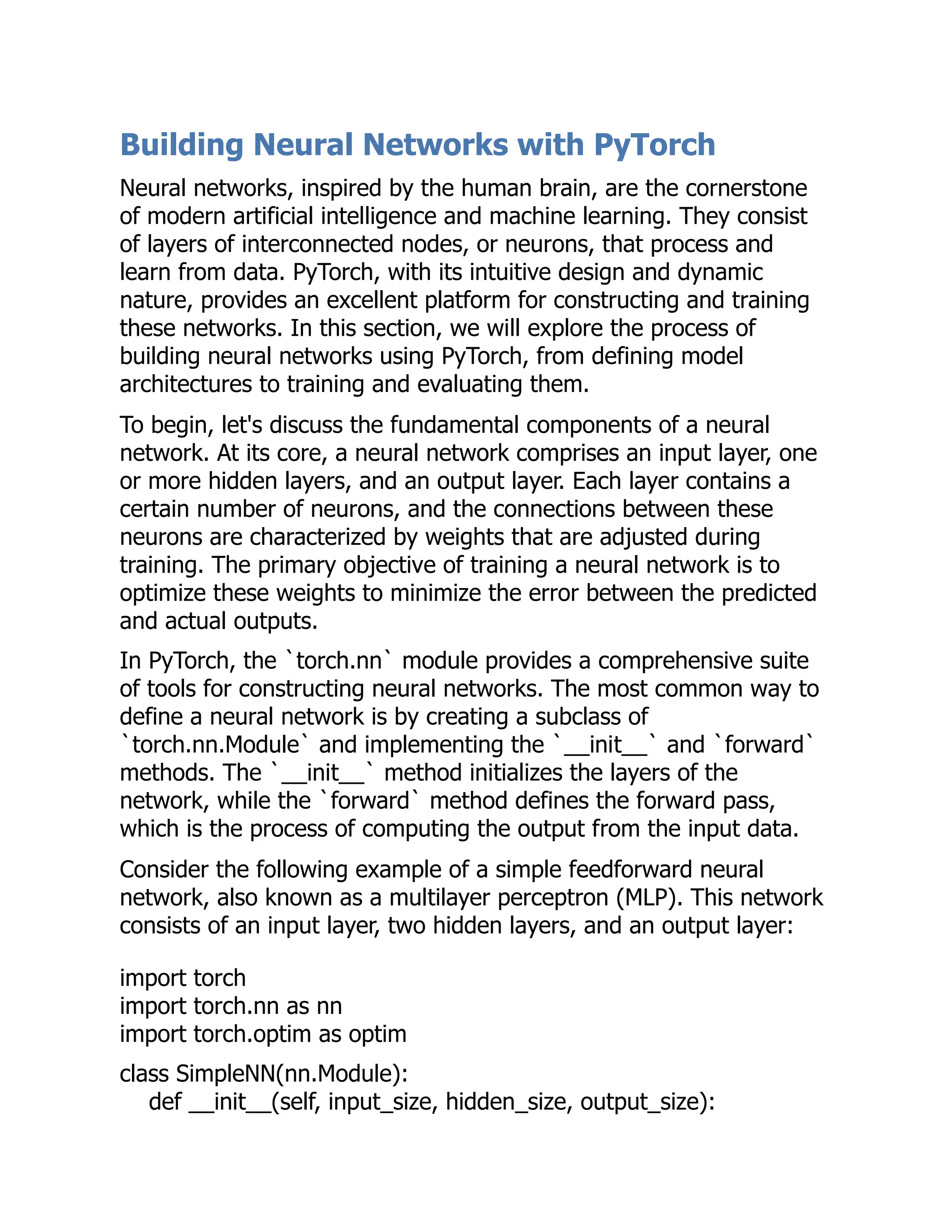
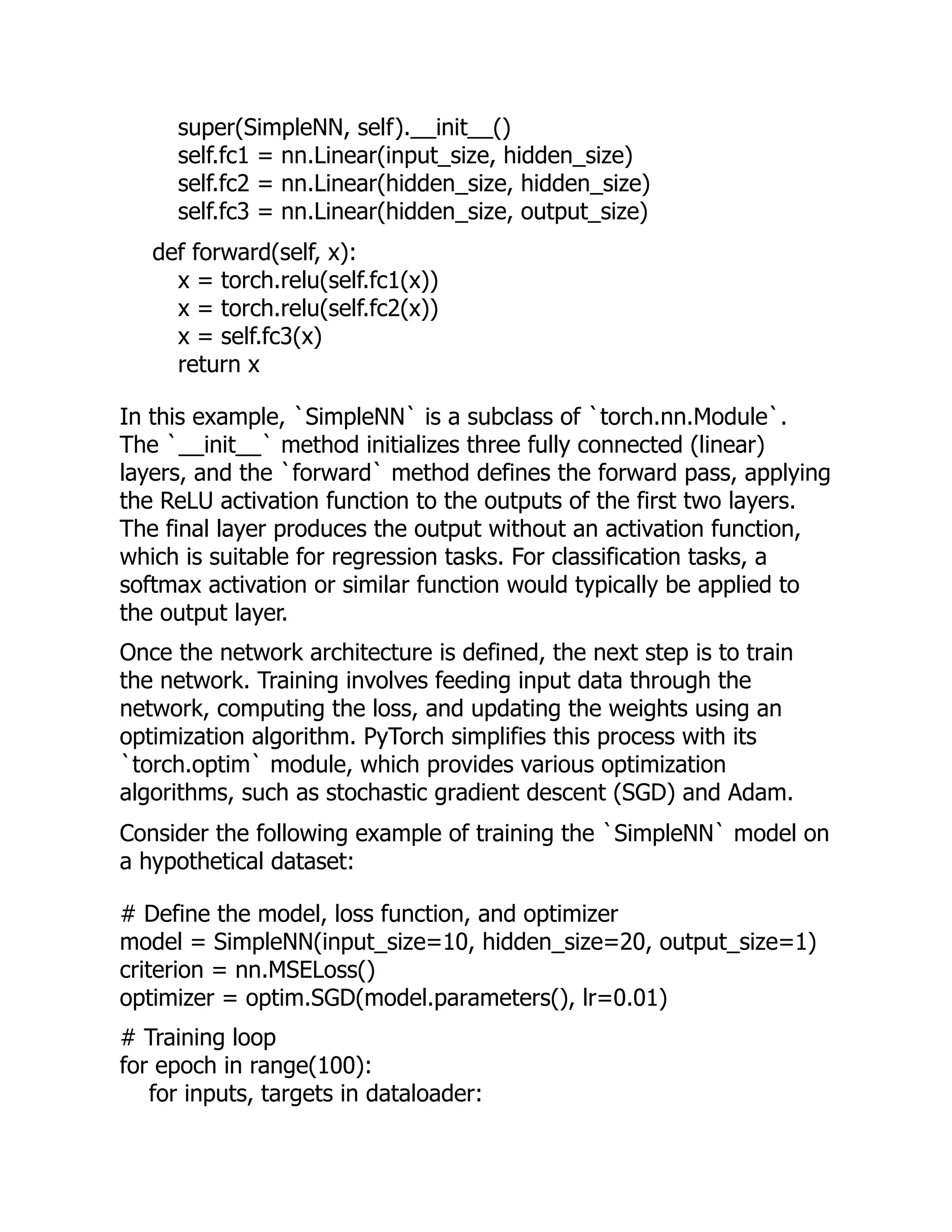
![# Zero the gradients
optimizer.zero_grad()
# Forward pass
outputs = model(inputs)
loss = criterion(outputs, targets)
# Backward pass and optimization
loss.backward()
optimizer.step()
print(f'Epoch [{epoch+1}/100], Loss: {loss.item()}')
In this example, we first define the model, loss function, and
optimizer. The `nn.MSELoss` function computes the mean squared
error loss, which is suitable for regression tasks. The `optim.SGD`
optimizer updates the model's parameters using stochastic gradient
descent with a learning rate of 0.01. The training loop iterates over
the dataset for a specified number of epochs, performing the
forward pass, computing the loss, performing the backward pass,
and updating the weights in each iteration.
Evaluating the performance of a trained neural network is crucial for
understanding its effectiveness. This typically involves measuring the
model's accuracy on a separate validation or test dataset. PyTorch
provides tools for computing various metrics, such as accuracy,
precision, and recall. Consider the following example of evaluating
the `SimpleNN` model:
# Evaluation mode
model.eval()
# Disable gradient computation
with torch.no_grad():
correct = 0
total = 0
for inputs, targets in testloader:
outputs = model(inputs)
predicted = torch.argmax(outputs, dim=1)](https://image.slidesharecdn.com/29152153-250523200457-8df50e1e/75/Pytorch-A-Detailed-Overview-Agladze-Mikhail-23-2048.jpg)
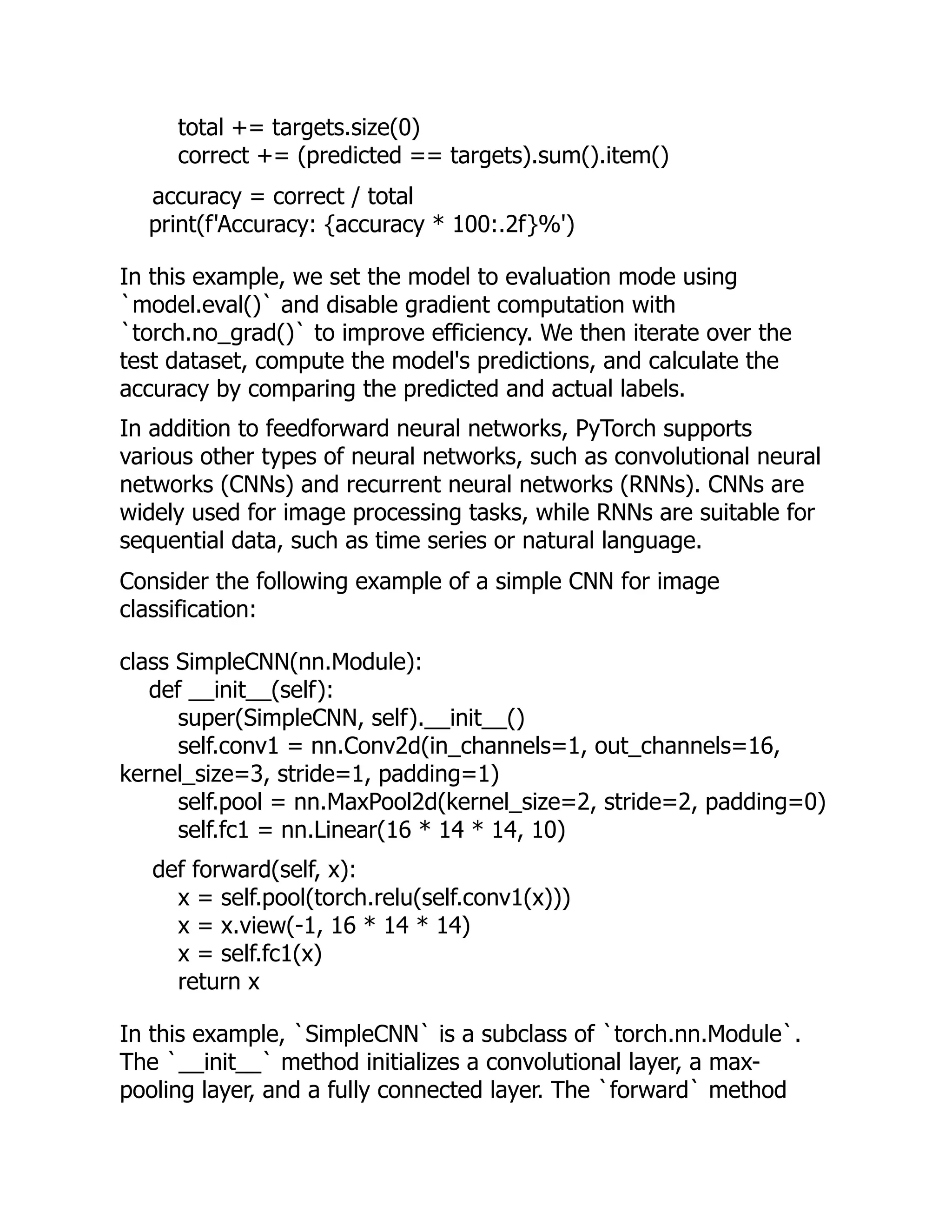
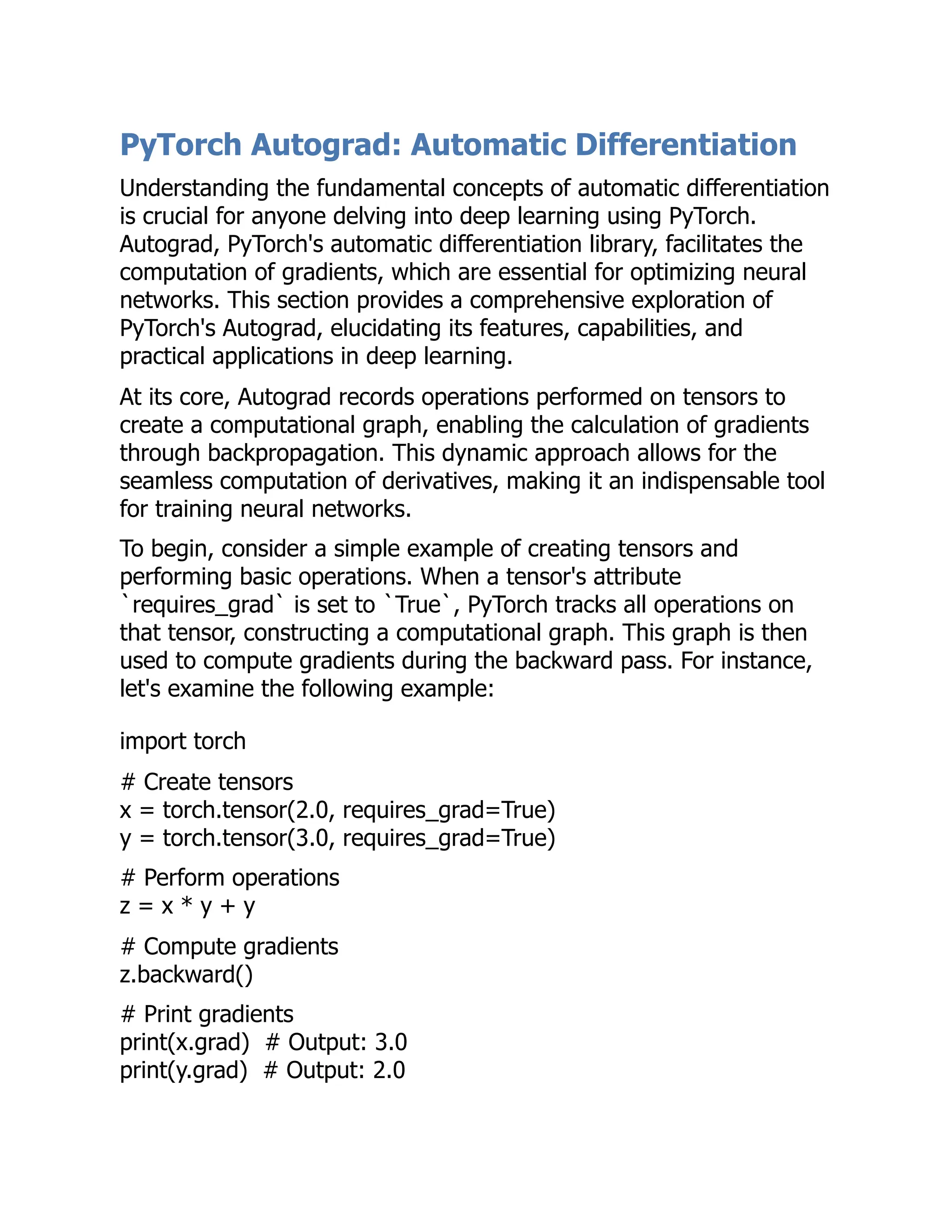
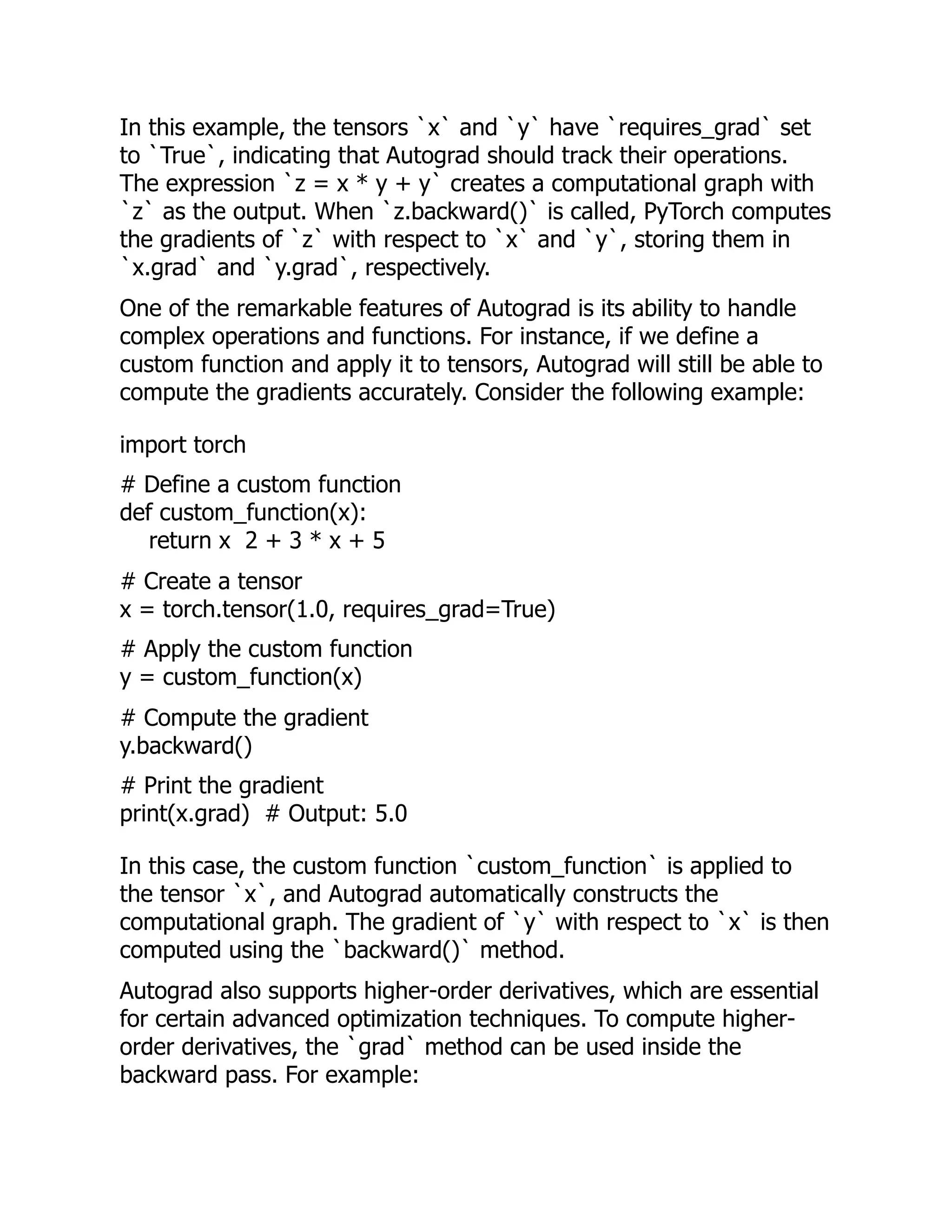
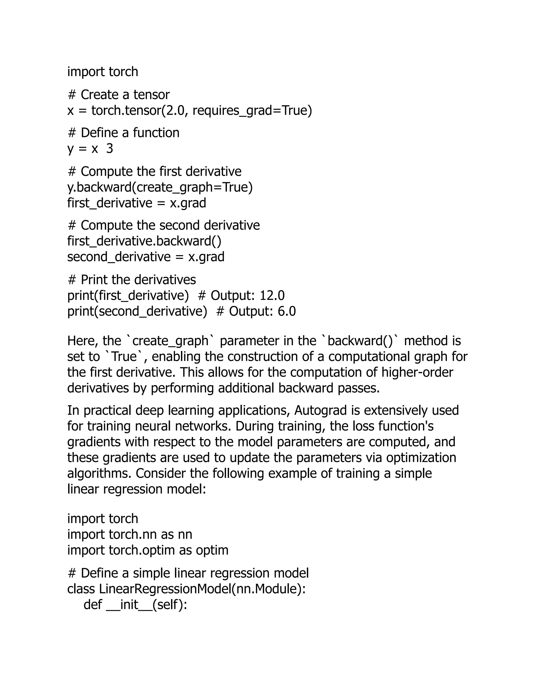
![super(LinearRegressionModel, self).__init__()
self.linear = nn.Linear(1, 1)
def forward(self, x):
return self.linear(x)
# Create a dataset
x_train = torch.tensor([[1.0], [2.0], [3.0]], requires_grad=True)
y_train = torch.tensor([[2.0], [4.0], [6.0]], requires_grad=True)
# Instantiate the model, loss function, and optimizer
model = LinearRegressionModel()
criterion = nn.MSELoss()
optimizer = optim.SGD(model.parameters(), lr=0.01)
# Training loop
for epoch in range(100):
# Zero the gradients
optimizer.zero_grad()
# Forward pass
outputs = model(x_train)
loss = criterion(outputs, y_train)
# Backward pass
loss.backward()
# Update the weights
optimizer.step()
# Print the final loss
print(loss.item())
In this example, the `LinearRegressionModel` is defined as a
subclass of `nn.Module`, and the training loop involves computing
the loss, performing the backward pass to calculate gradients, and
updating the model parameters using the optimizer. Autograd
automatically tracks the operations and computes the necessary
gradients during the backward pass.](https://image.slidesharecdn.com/29152153-250523200457-8df50e1e/75/Pytorch-A-Detailed-Overview-Agladze-Mikhail-29-2048.jpg)
![Another powerful feature of Autograd is its ability to handle non-
scalar outputs. In such cases, the `backward()` method requires an
additional argument to specify the gradient of the output with
respect to itself. For instance:
import torch
# Create a tensor
x = torch.tensor([[1.0, 2.0], [3.0, 4.0]], requires_grad=True)
# Define a function
y = x 2
# Compute the gradient
gradient = torch.ones_like(y)
y.backward(gradient)
# Print the gradient
print(x.grad)
Here, the tensor `y` has a non-scalar output, and the `backward()`
method is called with a gradient tensor of ones, enabling the
computation of gradients for each element in `x`.
To sum up, PyTorch's Autograd is a powerful and flexible library for
automatic differentiation, playing a pivotal role in the training of
neural networks. By dynamically constructing computational graphs
and efficiently computing gradients, Autograd simplifies the
optimization process and enables the development of complex deep
learning models. Mastering Autograd is essential for anyone looking
to harness the full potential of PyTorch in their deep learning
endeavors.](https://image.slidesharecdn.com/29152153-250523200457-8df50e1e/75/Pytorch-A-Detailed-Overview-Agladze-Mikhail-30-2048.jpg)
![Understanding and Using PyTorch Datasets
and DataLoaders
In deep learning, the preparation and handling of data are
paramount. PyTorch, a versatile and powerful deep learning
framework, provides robust tools to streamline this process through
its `torch.utils.data` module. This section will delve into the
intricacies of PyTorch Datasets and DataLoaders, elucidating their
roles, functionalities, and practical applications in deep learning
workflows.
To commence, let's explore the concept of a Dataset in PyTorch. A
Dataset is an abstract class representing a collection of data samples
and their corresponding labels. It serves as the foundation for data
handling in PyTorch, providing a standardized way to load and
preprocess data. By subclassing `torch.utils.data.Dataset`, users can
create custom datasets tailored to their specific needs.
Consider the following example of a custom Dataset class for a
hypothetical image classification task. This class loads images and
their labels from a directory, applies transformations, and returns the
processed data samples.
import os
from PIL import Image
import torch
from torch.utils.data import Dataset
from torchvision import transforms
class CustomImageDataset(Dataset):
def __init__(self, image_dir, transform=None):
self.image_dir = image_dir
self.transform = transform
self.image_paths = [os.path.join(image_dir, img) for img in
os.listdir(image_dir)]](https://image.slidesharecdn.com/29152153-250523200457-8df50e1e/75/Pytorch-A-Detailed-Overview-Agladze-Mikhail-31-2048.jpg)
![def __len__(self):
return len(self.image_paths)
def __getitem__(self, idx):
image_path = self.image_paths[idx]
image = Image.open(image_path)
if self.transform:
image = self.transform(image)
label = self._get_label_from_path(image_path)
return image, label
def _get_label_from_path(self, path):
# Placeholder function to extract label from the file path
return 0
In this example, the `CustomImageDataset` class is initialized with
the directory containing images and an optional transformation. The
`__len__` method returns the number of samples in the dataset,
while the `__getitem__` method retrieves an image and its label
based on the provided index. The `_get_label_from_path` function
is a placeholder for extracting labels from the file paths, which can
be customized as needed.
Transformations play a crucial role in preparing data for neural
network training. PyTorch's `torchvision.transforms` module offers a
variety of transformations, such as resizing, normalization, and data
augmentation. These transformations can be composed using
`transforms.Compose` and passed to the Dataset class. For
instance, the following code snippet demonstrates how to apply a
series of transformations to the images in the custom dataset.
transform = transforms.Compose([
transforms.Resize((128, 128)),
transforms.ToTensor(),
transforms.Normalize(mean=[0.5, 0.5, 0.5], std=[0.5, 0.5, 0.5])
])](https://image.slidesharecdn.com/29152153-250523200457-8df50e1e/75/Pytorch-A-Detailed-Overview-Agladze-Mikhail-32-2048.jpg)
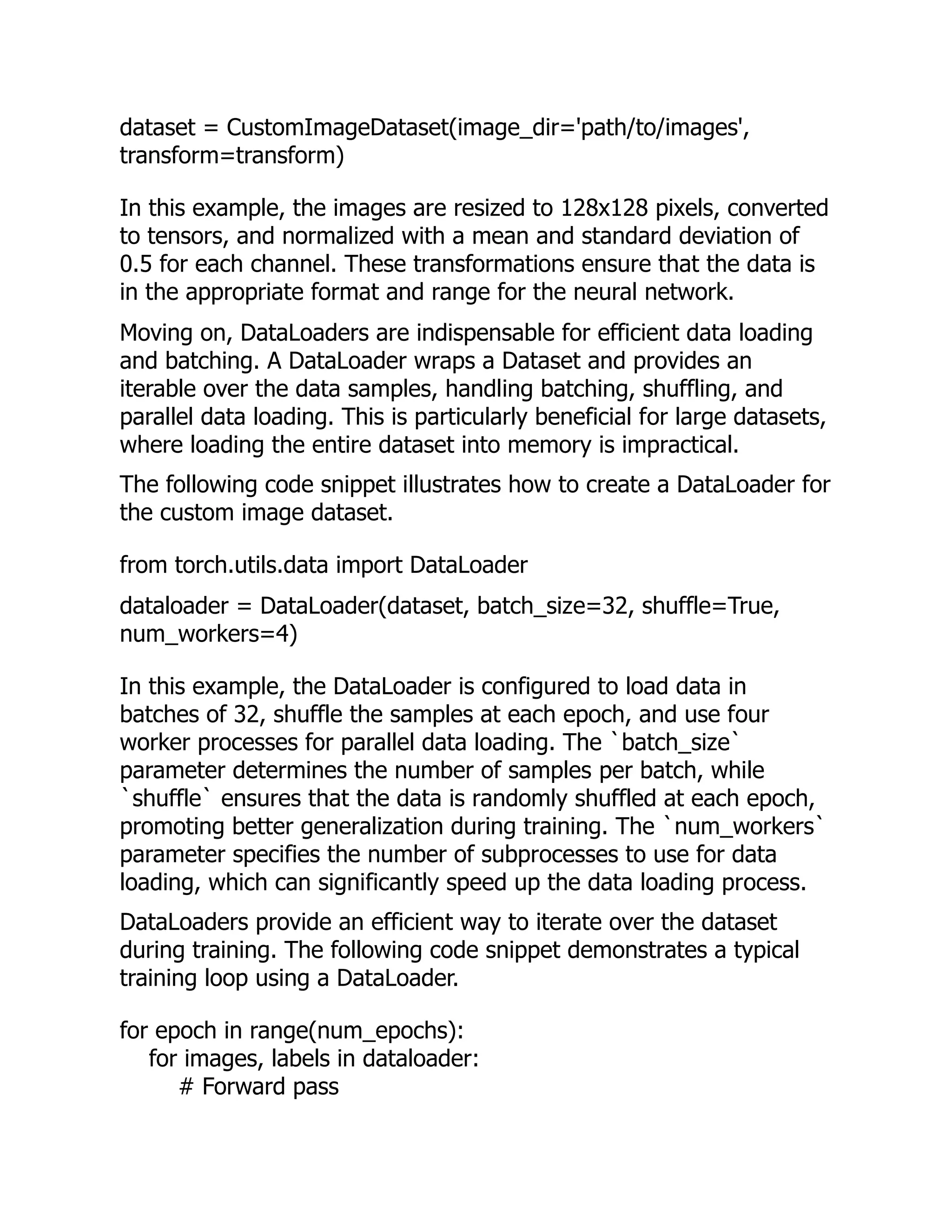
![outputs = model(images)
loss = criterion(outputs, labels)
# Backward pass and optimization
optimizer.zero_grad()
loss.backward()
optimizer.step()
print(f'Epoch [{epoch+1}/{num_epochs}], Loss: {loss.item()}')
In this example, the DataLoader iterates over the dataset, returning
batches of images and labels. The model performs a forward pass to
compute the outputs, and the loss is calculated using a predefined
criterion. The gradients are then computed via the backward pass,
and the optimizer updates the model parameters. This process is
repeated for the specified number of epochs, with the loss printed
after each epoch.
Furthermore, PyTorch supports built-in datasets for popular
benchmarks, such as CIFAR-10, MNIST, and ImageNet, through the
`torchvision.datasets` module. These datasets can be easily loaded
and used with DataLoaders, facilitating quick experimentation and
prototyping. For instance, the following code snippet demonstrates
how to load the CIFAR-10 dataset and create a DataLoader.
from torchvision.datasets import CIFAR10
cifar10_dataset = CIFAR10(root='path/to/data', train=True,
transform=transform, download=True)
cifar10_dataloader = DataLoader(cifar10_dataset, batch_size=32,
shuffle=True, num_workers=4)
In this example, the CIFAR-10 dataset is downloaded and
transformed using the specified transformations. A DataLoader is
then created to iterate over the dataset in batches.
In addition to standard datasets, PyTorch provides utilities for
handling data from various sources, such as text, audio, and video.
The `torchtext`, `torchaudio`, and `torchvision` libraries offer](https://image.slidesharecdn.com/29152153-250523200457-8df50e1e/75/Pytorch-A-Detailed-Overview-Agladze-Mikhail-34-2048.jpg)


![Iroqueses, cómo estaba organizada su Confederación, qué comieron,
cómo se vistieron y qué lengua hablaron; necesitamos saber,
además, lo que hicieron, la historia de sus trabajos, de sus luchas,
de sus heroísmos, de sus crueldades, de su aniquilamiento, de sus
acciones, en fin, y de la continuidad de sus efectos y sus causas. La
Arqueología, la Filología, la Ciencia política y demás auxiliares de la
Historia, dejan de lado aquellos acontecimientos que importan
acción, esa cualidad peculiarísima del hombre que usa el lenguaje, el
arte, el gobierno, las creencias, etc., como instrumentos para edificar
organismos sociales, para darles carácter y sello propio, para
producir sus cambios continuos y decidir su progreso ó
decadencia[1].
Los especialistas proporcionan los materiales, la piedra, el hierro, la
madera para construir el edificio. El historiador lo construye, recoge
los estudios de Filología Americana, de Arte Americano, de
Etnología, etc.; los reúne en un todo artístico proporcionado y
continuo, les da unidad y vida, y hace, en una palabra, Historia de
América.
Extensión y objeto.
2.—La Historia, no puede confundirse con la Sociología. Estudia esta
última la sociedad en general, su evolución y desarrollo, y el
verdadero objeto de la Historia, es el estudio de la unidad social, del
desenvolvimiento progresivo de la personalidad de un pueblo, raza ó
conjunto de pueblos que se desarrollan por el medio y la acción,
hasta perecer, ó constituir agrupaciones sociales definidas y
resistentes.
Tampoco puede limitarse el estudio de la Historia General de
América, á la del Continente Norte Americano, como han querido
algunos historiadores. Sud América tiene en la historia de la
civilización humana tanta ó más importancia que Norte América, y la
Raza Latina que puebla el Continente Sur, nada tiene que envidiar á](https://image.slidesharecdn.com/29152153-250523200457-8df50e1e/75/Pytorch-A-Detailed-Overview-Agladze-Mikhail-58-2048.jpg)
![la Sajona, que en general ocupa el Continente Norte. Las
agrupaciones indígenas más cultas y definidas, se formaron por otra
parte en la América del Sur. Prescindir del Continente Sud
Americano al estudiar la Historia General de América y llamar así á la
Historia Particular de los Estados Unidos, es tan ridículo como
estudiar, por ejemplo, la Historia de la llamada Edad Antigua,
prescindiendo de Roma ó de Grecia[2].
Consideraremos, pues, la Historia de América, en general,
estudiando la formación progresiva de las unidades sociales de sus
dos Continentes, procurando relacionarlas entre sí y comparar en
forma sintética las notas características de su respectivo desarrollo.
Divisiones.
3.—Para sistematizar en lo posible nuestro estudio, y sin pretensión
alguna dogmática, podemos dividir la Historia General de América en
cinco grandes Épocas.
1.ª América Indígena.—Abraza la Pre-historia y la historia
de la Raza Americana Primitiva hasta el Descubrimiento
Colombino.
2.ª Descubrimiento.—Abraza desde el primer viaje al
Continente Americano de Cristóbal Colón, hasta la vuelta á
España de Sebastián del Cano, después de su viaje de
Circunnavegación (1492-1518).
3.ª Conquista.—Estudia el conflicto de la Raza Indígena con
los Europeos, hasta su dominación por éstos y formación
definitiva de las diversas Colonias.
4.ª América Colonial.—Estudia el desarrollo cultural y
político de tales Colonias hasta los primeros síntomas de su
Independencia.](https://image.slidesharecdn.com/29152153-250523200457-8df50e1e/75/Pytorch-A-Detailed-Overview-Agladze-Mikhail-59-2048.jpg)
![5.ª La Independencia.—Comprende desde estos síntomas
de Independencia hasta la formación de las diversas
Nacionalidades Americanas[3].
Las Fuentes.
4.—Los materiales originales que sirven á los historiadores para
construir sus relaciones, se llaman fuentes. Corresponden á los
fósiles en geología, á los casos en los estudios legales, á las palabras
en filología, etc., etc. Son restos del pasado, de donde se deriva el
conocimiento del mismo. Consisten en la masa de tradiciones,
manuscritos, impresos, monumentos, restos, útiles, instituciones,
literaturas, etc., en las que una generación, pueblo ó raza se
exterioriza tangible y visiblemente. Todo lo que nuestros
antepasados nos legaron, sus instituciones, sus creencias, sus leyes,
su lengua, sus edificios, sus industrias, etcétera, son fuentes de su
historia, que no pueden confundirse con la historia misma que con
ellos formaron sus cronistas, omitiendo á veces ó exagerando, lo que
creían dañoso ó conveniente para mantener su punto de vista
religioso, social ó político. La Historia encuentra en las fuentes,
materiales de toda especie siempre utilizables. El contenido y la
dirección de la historia, cambian con las generaciones; las fuentes
permanecen y perduran. Tienen vividez, sello propio y particular
encanto. Son las progenitoras de la historia. Ellas deben resolver
toda controversia, y en ellas deben fundarse todas las crónicas.
Archivos y Museos.
5.—Así como para estudiar la Botánica, la Zoología, etc., debe
acudirse á los Museos de Ciencias Naturales, donde se han reunido
ejemplares diversos para estudiar la civilización de las sociedades
humanas, es convenientísimo visitar los Museos Etnológicos,
Arqueológicos, Históricos, etc., en los que se guardan](https://image.slidesharecdn.com/29152153-250523200457-8df50e1e/75/Pytorch-A-Detailed-Overview-Agladze-Mikhail-60-2048.jpg)
![cuidadosamente clasificados los restos, reliquias, útiles,
herramientas, orfebrerías, ornamentos, etc., que juntamente con los
monumentos arquitectónicos (edificios, caminos, acueductos,
templos, ruinas, etc.), nos dan á veces clarísima idea del vivir
cultural de pasados pueblos. Los repositorios más ricos en
Antigüedades Americanas son, entre otros, el Peabody Museum, de
Cambridge, Mass. (E. U.), las colecciones de la Smithsonian
Institution, y de la Oficina de Etnología de Washington (E. U.), el
Museo Nacional de Washington, las colecciones Etnológicas del
Museo Británico, del Königliche Museum, de Berlín, y del Museo
Etnográfico, de San Petersburgo; el Museo Arqueológico, de Madrid;
el Museo Nacional, de México; el Museo de la Plata, el Museo
Nacional, de Buenos Aires; el de Río Janeiro, Santiago de Chile, etc.,
etc. Casi todos estos Museos han publicado, y siguen publicando en
sus anales, revistas y catálogos, reproducciones artísticas y fieles de
sus tesoros Arqueológicos[4].
Las fuentes manuscritas, y en especial las de carácter oficial, se
guardan cuidadosamente en sus Archivos por todas las naciones
cultas. Estando la Historia Americana íntimamente relacionada con la
Europea, apenas hay Archivo importante en Europa que no contenga
fuentes manuscritas interesantes para el Historiador de América.
Claro es que los Archivos Españoles, Portugueses, Ingleses y
Franceses, son los más ricos de Europa en documentación
Americana. Toda la Historia Colonial de las actuales Repúblicas
Hispano-Americanas, por ejemplo, puede y debe estudiarse en los
Archivos Españoles.
En las Referencias de este Compendio se mencionan especialmente
los Archivos que contienen las principales fuentes manuscritas de
cada una de sus materias y capítulos[5].
Colecciones de documentos.](https://image.slidesharecdn.com/29152153-250523200457-8df50e1e/75/Pytorch-A-Detailed-Overview-Agladze-Mikhail-61-2048.jpg)
![6.—Para que las fuentes manuscritas de la Historia se conozcan sin
necesidad de visitar los distintos Archivos, y para hacerlas además
fácilmente inteligibles para los profanos en las disciplinas
paleográficas, deben coleccionarse y publicarse.
Desde el principio del siglo xviii, todas las naciones Europeas han
procurado coleccionar, y han coleccionado y publicado casi todas las
fuentes de su historia. Como gran parte de estas colecciones son
sólo accesibles en las grandes Bibliotecas, para mayor facilidad del
estudioso se han empezado también á publicar en estos últimos
años en muchas naciones de Europa y en algunas de las
Americanas, colecciones populares de fuentes, clasificadas según su
importancia y sus épocas. La utilidad de estos elementales
instrumentos de investigación histórica es grandísima, tanto por la
facilidad de su adquisición como por la sencillez de su manejo.
El cuidadoso estudio de las fuentes ha dado además origen á
disciplinas científicas nuevas (Filología, Paleografía, Eurística,
Diplomática, etc.), que exigen á su vez nuevas escuelas y aparatos
científicos. El modelo de estas nuevas escuelas ó talleres históricos
es el Seminarium alemán, cuyos únicos materiales de trabajo son las
fuentes, y en el que los estudiantes investigan por sí mismos,
construyendo con las referidas fuentes trabajos históricos originales.
Algunas Universidades Norte-Americanas; la Ecole de Cartes, de
París; el Centro Arabista, de Madrid y otras instituciones de
investigación histórica, han adoptado el acertadísimo sistema del
Seminarium, de Alemania, ampliando un tanto su criterio[6].
Las Autoridades.
7.—Entendemos por Autoridades, las monografías, tratados ó libros
de historia, basados en las fuentes. Si no se hubiera escrito, por
ejemplo, ninguna historia del General San Martín, tendría que
recurrir el que la escribiera, á los diversos Archivos, para buscar las
fuentes originales de información; más aún, debería mencionarlas en](https://image.slidesharecdn.com/29152153-250523200457-8df50e1e/75/Pytorch-A-Detailed-Overview-Agladze-Mikhail-62-2048.jpg)
![originales y los trabajos modernos que deben consultarse sobre una
época ó punto históricos, (Bibliografía Retrospectiva), ó sólo los
trabajos modernos (Bibliografía Corriente), clasificándose estos
últimos según comprendan la Historia Universal, la Nacional, la
Regional, ó alguna rama especial de la Historia.
Desgraciadamente, no existe un Repertorio General Bibliográfico de
la Historia Americana. Los publicados en los Estados Unidos, por
todos conceptos notables y útiles, tienen un carácter netamente
nacional. El historiador de Sud América tiene necesariamente que
formar su propio Repertorio Bibliográfico, y recurrir para ello á los
meritorios trabajos aislados de algunos eruditos, que en su lugar se
mencionarán, á las antiguas Bibliografías Retrospectivas, á los
Catálogos de las Bibliotecas Públicas Sud-Americanas, á los
generales de las grandes Bibliotecas Europeas (Museo Británico,
Nacional de París, etcétera), á los de las Bibliotecas Españolas
(Nacional, Colombina, de Palacio, Escorialense, de la Academia de la
Historia, del Museo de Ultramar, etc.), á las publicaciones,
Repertorios, Enciclopedias, Boletines y Revistas Históricas y
Bibliográficas, etc, etc. A falta de algo mejor y más completo, el
conjunto de las "Referencias" de mi Compendio puede servir de
Manual ó Guía elementalísima, de la Bibliografía General del
Continente Americano[7].
Mapas y estudios fisiográficos.
9.—Parece inútil acentuar la íntima y necesaria relación de la
Geografía con la Historia. Mal pueden estudiarse el desarrollo y
formación de las nacionalidades y pueblos Sud-Americanos, sin
conocer exactamente las regiones y lugares que sucesivamente
fueron ocupando. La Cartografía Histórica de América, es elemento
indispensable para el estudio de su historia. Las relaciones de los
primeros exploradores, conquistadores y misioneros, los mapas de
los antiguos cartógrafos, las concesiones de las diversas naciones
Europeas para fundar colonias, los tratados de límites, las decisiones](https://image.slidesharecdn.com/29152153-250523200457-8df50e1e/75/Pytorch-A-Detailed-Overview-Agladze-Mikhail-64-2048.jpg)
![lagos, las producciones forestales y agrícolas, la fauna y la flora
Americana, han influenciado decididamente su evolución histórica. El
estudio de dichos rasgos fisiográficos nos da las más de las veces la
clave y la causa de acontecimientos históricos á primera vista
casuales ó inexplicables[8].
Metodología.
10.—De lo anteriormente expresado puede fácilmente deducirse los
Métodos que deben adoptarse para el estudio de la Historia General
de América. Entiéndese por método, el orden que se sigue en las
diversas ciencias para hallar y enseñar la verdad. Dependiendo la
verdad histórica de la evidencia humana, claro es que para hallarla
deben observarse las reglas lógicas que depuran y acrisolan
semejante evidencia. El historiador es una especie de Juez de
Instrucción, que reúne pruebas documentales, etc., de los hechos
que examina. Debe verificar, por tanto, el texto de sus documentos
probatorios (Crítica de restitución), saber de dónde proceden,
(Crítica de origen), clasificarlos, relacionarlos con otros, y con las
autoridades, interpretarlos, y ejercer su sentido crítico para
averiguar la sinceridad ó insinceridad de sus autores (Crítica
interna). Realizadas estas operaciones analíticas, debe sintetizar sus
resultados, agrupar los hechos, llenar las lagunas que dejaren,
según su sano razonar crítico, y construir, por fin, su informe ó
relación histórica, huyendo de toda parcialidad y filosófico prejuicio.
No es posible establecer reglas generales de interpretación. Depende
del sentido crítico de los historiadores, de su erudición, de sus
condiciones intelectuales, de su concentración ó de su esfuerzo. Con
idénticos métodos pueden llegarse á interpretaciones distintas. El
método y las fuentes son para todos iguales; la interpretación es
personalísima. "El Criterio", de Balmes, y el "Tratado de las Pruebas",
de Jeremías Bentham, son (á mi juicio) normas inapreciables de
Metodología. Su atenta lectura basta para enseñarnos la técnica
histórica, el modo de investigar y apreciar evidencias. No pueden](https://image.slidesharecdn.com/29152153-250523200457-8df50e1e/75/Pytorch-A-Detailed-Overview-Agladze-Mikhail-66-2048.jpg)
![enseñarnos, sin embargo, á hacer la historia, á componer con
brillantez y hondura una monografía ó un libro. Reside tal facultad
en el historiador mismo. Si es, por ejemplo, un Parkman,
coleccionará primero todas las Relaciones de los Misioneros Jesuítas,
elegirá las que al antiguo Canadá se refieren, entre éstas las de los
misioneros más celosos, más observadores y que más tiempo
estuvieron en aquellas tierras, y depurándolas, relacionándolas é
interpretándolas con sinceridad y elevado espíritu, legará al mundo
moderno ese modelo de autoridades históricas, esa epopeya de
abnegaciones y heroísmos que se llama "Los Jesuítas en Norte
América".
La Historia no está ya destinada á dormir, mientras los manuales de
cuarta ó quinta mano y los maestros superficiales y dogmáticos
cuentan hechos aprendidos de memoria á sus alumnos inatentos.
Debe despertar y entrar á la vida. El pasado vive en el presente.
Observando con atención lo actual y vivido, discerniremos más
fácilmente las formas, ideas é instituciones de lo pretérito. Así como
las Ciencias Naturales han salido de los estrechos límites del libro de
texto para entrar al mundo de los fenómenos, de los Laboratorios y
de los Museos, así la Historia debe independizarse de
memorizaciones y viejas disciplinas escolares, entrar al mundo de la
naturaleza humana, y abandonar las antiguas aulas por Seminarios
especiales, dotados de mapas, colecciones de fuentes, autoridades,
etc., etc., en los que cada estudiante, guiado por un Maestro que
con él trabaje, interprete por sí mismo los materiales históricos y
ejercite su espíritu crítico. Así y sólo así, podrá alcanzarse el ideal de
la enseñanza histórica y podrá inculcarse en los alumnos el deseo de
ver, sentir y verificar con su inteligencia y su trabajo, lo ético y
luminoso de la VERDAD y el PATRIOTISMO[9].](https://image.slidesharecdn.com/29152153-250523200457-8df50e1e/75/Pytorch-A-Detailed-Overview-Agladze-Mikhail-67-2048.jpg)
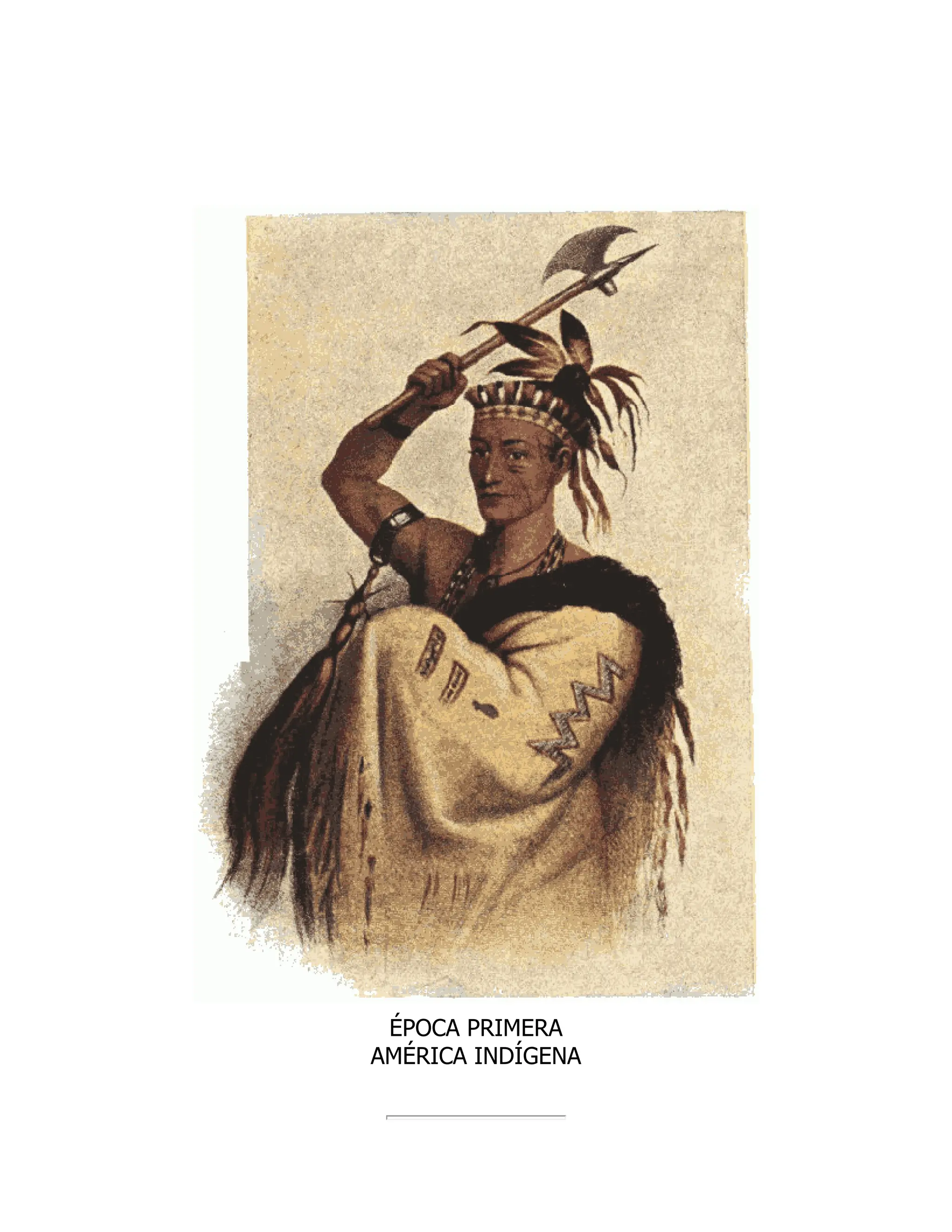

![1.—Desde la creación del hombre[10] hasta el primer testimonio
escrito de su vivir histórico, hay un período obscuro y de duración
variable, que designar podemos con el nombre de Prehistórico[11].
Fig. 1.—Corte estratigráfico. Hancock (Virginia E. U.)
No existe crónica alguna de lo acaecido en América antes de ser
descubierta por Colón. Las inscripciones y códices indígenas que han
llegado hasta nosotros, no han podido todavía descifrarse con
certeza. La historia del Continente Americano empieza, pues, al
finalizar el siglo xv. Todo lo anterior á dicha fecha pertenece en
América al campo de lo prehistórico[12].
Hay un hecho cierto que sirve de punto de partida para investigar
tan obscuras épocas. Al llegar los conquistadores europeos á las
costas de América encontraron en ellas hombres que creyeron
distintos de los del Continente Antiguo, pueblos extraños de
organización peculiarísima. ¿De dónde venían? ¿Cuál fué su origen y
cuál su antigüedad? Los guerreros del siglo xv y xvi no pudieron
averiguarlo. Los datos obtenidos hasta hoy por la ciencia son
también insuficientes para esclarecer el enigma.](https://image.slidesharecdn.com/29152153-250523200457-8df50e1e/75/Pytorch-A-Detailed-Overview-Agladze-Mikhail-71-2048.jpg)
![Fig. 2.—Formación glacial. Isla Sebree (Alaska).
Nos limitaremos, pues, á plantear tan obscuros problemas sin
pretender resolverlos, y á relacionar sumariamente los datos ó
fragmentos de dato que la Arqueología y la Etnología[13] pueden
proporcionarnos.
Materiales para su estudio.
2.—La fuente principal para el estudio de lo prehistórico está en los
monumentos, útiles y objetos paleográficos que de los primitivos
Americanos han llegado hasta nosotros. Como productos
indiscutibles de sus actividades nos ayudan á conocer sus ideas,
costumbres y cultura. El estudio y comparación de las lenguas y
dialectos Americanos nos permite también determinar la afinidad de
tribus separadas geográficamente y trazar el probable curso de sus
emigraciones y movimientos. Las tradiciones y leyendas nos
proporcionan, por último, valiosos datos que corroboran
conclusiones dudosas ó aniquilan teorías inciertas.](https://image.slidesharecdn.com/29152153-250523200457-8df50e1e/75/Pytorch-A-Detailed-Overview-Agladze-Mikhail-72-2048.jpg)
![Fig. 3.—Precipicios y glaciares del Aconcagua (Chile).
Las edades geológicas.
3.—Los materiales que componen la corteza terrestre no están
amontonados en caprichoso desorden, sino dispuestos en lechos ó
estratos sucesivos colocados en el orden en que se fueron formando.
Basados en esta ley de superposición estratigráfica, aplicable á todas
las regiones del globo[14], han dividido los geólogos el proceso de
formación de la tierra en edades y períodos de duración cronológica
incierta, caracterizados por la estructura de las rocas que componen
los estratos superpuestos[15].
Los períodos glaciales.
4.—El más interesante de los episodios geológicos de la edad
cuaternaria, única que interesa á nuestro estudio, es el avance y
retroceso de las enormes sábanas de hielo que en períodos
sucesivos, llamados glaciales, invadieron las regiones septentrionales
de Europa y América[16], allanando los montes, transformando los
valles, arrastrando, estriando ó pulimentando las rocas y acarreando](https://image.slidesharecdn.com/29152153-250523200457-8df50e1e/75/Pytorch-A-Detailed-Overview-Agladze-Mikhail-73-2048.jpg)
![piedras y arenas, para amontonarlas al retroceder en depósitos
geológicos de estructuras complejas y formas características[17].
Acumuláronse tales depósitos en algunos ríos á manera de bancos, y
convirtieron en extensos lagos los primitivos valles. Desviaron otros
ríos su curso, buscando nuevos cauces y formando gargantas
profundas. La humedad atmosférica, el descenso de la temperatura
y la acción misma de los glaciales, ocasionaron también
extraordinarios cambios en la faz de la vida orgánica, haciendo
desaparecer algunas especies animales y vegetales y emigrar á otras
á regiones diversas.
Fig. 4.—Formaciones fósiles (Pentacrinus Hiemeri) Museo Británico
(Nat. Hist.)
Las causas[18], fecha y duración de los períodos glaciales, no se
conoce con certeza. Parece, sin embargo, demostrado, que el](https://image.slidesharecdn.com/29152153-250523200457-8df50e1e/75/Pytorch-A-Detailed-Overview-Agladze-Mikhail-74-2048.jpg)
![principio y fin de los mismos es relativamente reciente[19]
(cuaternario-pleistoceno), y que el avance de los hielos sobrevino en
dos épocas distintas y separadas por largos intervalos de más alta
temperatura que estacionaron los glaciales en las altas mesetas y en
las regiones árticas y antárticas[20].
Fig. 5.—Formación fósil carbonífera de Iowa (E. U.) Museo Británico
(Nat. Hist.)](https://image.slidesharecdn.com/29152153-250523200457-8df50e1e/75/Pytorch-A-Detailed-Overview-Agladze-Mikhail-75-2048.jpg)
![Fig. 6.—Esqueleto fósil del Jetiosauro marino (Ichthyosaurian
termirostris). Museo Británico (Nat. Hist.)
La ley de Asociación.
5.—La sucesión, emigración y evolución de los organismos animales
fósiles ha podido asociarse con las edades geológicas en que
predominaron y en general caracterizan, llegando al convencimiento
de que el conjunto de fósiles de un estrato geológico dado, difiere
del de los estratos inferiores ó más antiguos y superiores ó más
modernos. En tales principios científicos se funda la llamada Ley de
Asociación.[21]](https://image.slidesharecdn.com/29152153-250523200457-8df50e1e/75/Pytorch-A-Detailed-Overview-Agladze-Mikhail-76-2048.jpg)
![Fig. 7.--El dinosauro unicornio (Triceratops-Prorsus de _Marsh_).
Limitándonos á los fósiles cuaternarios[22], podemos en general
afirmar que en la misma edad geológica en que vivieron el oso y el
león de las cavernas, el mastodonte, etc., en el continente Europeo,
existieron en el Americano el megaterio, el mylodon, el glyptodon, el
megalonix[23] y demás especies animales gigantescas, ya
extinguidas[24], cuyos esqueletos reconstruídos admiramos en los
Museos[25].
Criterios arqueológicos.
6.—El hombre, ser dotado de razón y libertad, aparece sobre la
tierra en la edad geológica cuaternaria[26]. Para satisfacer las
necesidades físicas y defenderse de las fieras é inclemencias
atmosféricas[27], necesitó valerse de herramientas y útiles y buscar
ó construir refugios más ó menos invulnerables.](https://image.slidesharecdn.com/29152153-250523200457-8df50e1e/75/Pytorch-A-Detailed-Overview-Agladze-Mikhail-77-2048.jpg)
![Fig. 8.—El Allosaurus (Reconstrucción C. R. Knight) American
Museum (U. S.)
La observación del estilo y forma de estas herramientas, útiles y
refugios, concordada con la de los estratos geológicos en que se
encuentren (superposición), y los restos humanos y de animales
extinguidos que en dichos estratos les acompañen, (asociación), son
los únicos cánones que pueden conducirnos á esclarecer en lo
posible el intrincado problema de la antigüedad del hombre en
América[28].](https://image.slidesharecdn.com/29152153-250523200457-8df50e1e/75/Pytorch-A-Detailed-Overview-Agladze-Mikhail-78-2048.jpg)
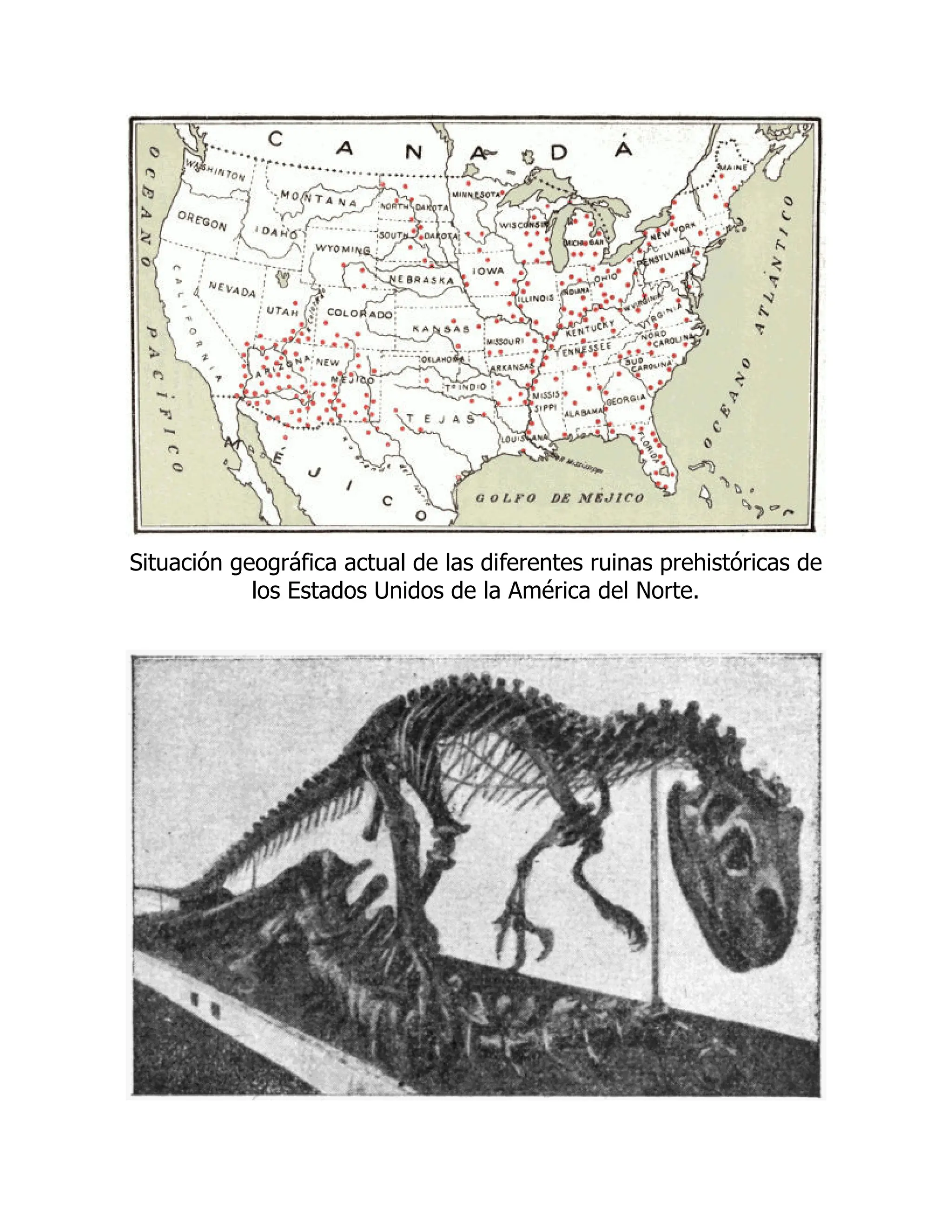
![Fig. 9.—Esqueleto reconstruído del Allosaurus sobre el del
Brontosaurus (Am. Mus. U. S.)
Los arqueólogos Europeos,[29] basados en el estilo y material de los
restos arqueológicos, distinguen en los tiempos prehistóricos las tres
célebres edades de la piedra, del bronce y del hierro[30],
subdividiendo la primera, ó lítica, en varias épocas. Eolítica, ó de la
piedra cortada, paleolítica, ó de la tallada y neolítica, ó de la
pulimentada, según el grado de perfección que alcanzaron en las
diversas localidades los referidos útiles líticos.
Fig. 10.--Reptil Dinosaurio (Diplodocus carnegii de Wyoming U. S. A.)
(Museo Británico).
La ausencia del hierro y en general del bronce entre los indígenas
Americanos, excluyen hasta hoy de su prehistoria las dos últimas
edades. América no conoció el hierro hasta la llegada de Colón. Los
indios de América del Norte y gran parte de los de la del Sur no](https://image.slidesharecdn.com/29152153-250523200457-8df50e1e/75/Pytorch-A-Detailed-Overview-Agladze-Mikhail-80-2048.jpg)
![conocieron el bronce[31], y la edad del cobre que algunos
arqueólogos han querido equiparar en América á la del bronce
Europea, no ha podido determinarse con certeza[32].
Fig. 11.—Dinosauro Acorazado (Stegosaurus ungulatus) O. C. Marsh.
(Universidad de Yale. E. U.)
Por otra parte, aun existiendo en el Continente Americano pruebas
abundantes de las culturas líticas, no es posible aplicar estrictamente
la división en épocas paleolíticas y neolíticas. Aceptaremos, pues,
tales términos sólo como descriptivos, procurando alejar de nuestra
mente toda idea de tiempo para sustituirla con la de sucesión ó
progreso[33].
Útiles paleolíticos.
7.—Llamaremos útiles paleolíticos, á aquellos objetos rudos de
piedra de variados tamaños y grosera talla que hayan sido
encontrados en lechos geológicos indudablemente pleistocenos ó](https://image.slidesharecdn.com/29152153-250523200457-8df50e1e/75/Pytorch-A-Detailed-Overview-Agladze-Mikhail-81-2048.jpg)


![[Update] PyTorch Tutorial for NTU Machine Learing Course 2017](https://cdn.slidesharecdn.com/ss_thumbnails/pytorchtutorial-2017-1103-171103060015-thumbnail.jpg?width=640&height=640&fit=bounds)