Download as PDF, PPTX


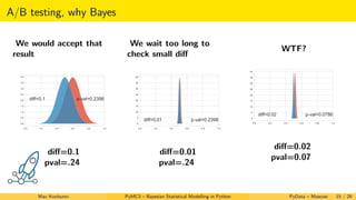
![Hierarchical Models
What if we have more diverse data? We can estimate an amount of devils + uncertainty!
Data: [8, 2, 2, 10, 0,
0, 2, 5, 6, 10] out of 20 flips
λDevil ∼ Exponential(1)
λAngel ∼ Exponential(1)
pi ∼ Beta(λAngel , λAngel + λDevil )
flipsi ∼ Binomial(pi , Ni )
Max Kochurov PyMC3 – Bayesian Statistical Modelling in Python PyData – Moscow 8 / 29](https://image.slidesharecdn.com/6-190715100351/85/PyMC3-Bayesian-Statistical-Modelling-in-Python-22-2019-22-320.jpg)
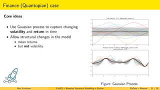
![Hierarchical Models
What if we have more diverse data? We can estimate an amount of devils + uncertainty!
Data: [8, 2, 2, 10, 0,
0, 2, 5, 6, 10] out of 20 flips
λDevil ∼ Exponential(1)
λAngel ∼ Exponential(1)
pi ∼ Beta(λAngel , λAngel + λDevil )
flipsi ∼ Binomial(pi , Ni )
Max Kochurov PyMC3 – Bayesian Statistical Modelling in Python PyData – Moscow 8 / 29](https://image.slidesharecdn.com/6-190715100351/85/PyMC3-Bayesian-Statistical-Modelling-in-Python-22-2019-23-320.jpg)


![Inspecting Your Model
plt.hist(trace["angels"],
alpha=.8, label='Alpha')
plt.hist(trace["angels"]+trace["devils"],
alpha=.8, label='Beta')
plt.legend(fontsize=20)
0 1 2 3 4 5 6 7 8
0
50
100
150
200
250
300
Alpha
Beta
Max Kochurov PyMC3 – Bayesian Statistical Modelling in Python PyData – Moscow 11 / 29](https://image.slidesharecdn.com/6-190715100351/85/PyMC3-Bayesian-Statistical-Modelling-in-Python-22-2019-28-320.jpg)
![Inspecting Your Model
0.0 0.2 0.4 0.6 0.8 1.0
0
1
2
3
4
5
6
7
Prob Distribution
for a, b in zip(
trace["angels"],
trace["angels"]+trace["devils"]
):
plt.plot(
np.linspace(0, 1),
st.beta(a, b).pdf(np.linspace(0, 1)),
color="b", alpha=.025
)
a_mean = trace["angels"].mean()
b_mean = (trace["angels"]+trace["devils"]).mean()
plt.plot(
np.linspace(0, 1),
st.beta(a_mean, b_mean).pdf(np.linspace(0, 1)),
color="black", linewidth=4.0
)
plt.axvline(0.5)
plt.title("Prob Distribution", fontsize=20)
Max Kochurov PyMC3 – Bayesian Statistical Modelling in Python PyData – Moscow 12 / 29](https://image.slidesharecdn.com/6-190715100351/85/PyMC3-Bayesian-Statistical-Modelling-in-Python-22-2019-29-320.jpg)


The document introduces PyMC3 for Bayesian statistical modeling in Python, explaining the basics of Bayesian statistics including prior, likelihood, and posterior concepts. It discusses the application of Bayesian inference in various fields such as finance, music streaming, e-commerce, astronomy, life sciences, and medicine. Furthermore, it covers Markov Chain Monte Carlo (MCMC) methods, hierarchical models, and case studies including A/B testing, highlighting the advantages of Bayesian approaches over traditional frequentist methods.


![Mapping Lo Dto Proton Revised [Compatibility Mode]](https://cdn.slidesharecdn.com/ss_thumbnails/mappinglodtoprotonrevisedcompatibilitymode-1289121936987-phpapp01-thumbnail.jpg?width=640&height=640&fit=bounds)


![[P.D.F] Bayesian Methods for Hackers: Probabilistic Programming and Bayesian ...](https://cdn.slidesharecdn.com/ss_thumbnails/bayesian-methods-for-hackers-probabilistic-programming-and-bayesian-inference-191119012050-thumbnail.jpg?width=640&height=640&fit=bounds)


![Lect 1 Number systems and base conversions. [Autosaved].pptx](https://cdn.slidesharecdn.com/ss_thumbnails/lect1numbersystemsandbaseconversions-260111134109-67c2d865-thumbnail.jpg?width=640&height=640&fit=bounds)


