
Recommended
More Related Content
Featured
Featured (20)
Prova finale di econometria applicata
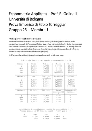
- 1. 1 Econometria Applicata - Prof. R. Golinelli Università di Bologna Prova Empirica di Fabio Torreggiani Gruppo 25 - Membri: 1 Prima parte - Dati Cross-Section Relazione di interesse: effetto sulla produzione di vino (variabile q) esercitato dall’abiltà manageriale (manag), dall’impiego di fattore lavoro (lab) e di capitale (cap). I dati si riferiscono ad una cross-section di N=74 imprese per l’anno 2010. Non si conosce la misura di manag, ma si ha una sua misura approssimativa: il numero di anni di esperienza dei manager (xper). Infine, nel modello si dispone anche dell’età del manager (age). 1 - Effettuare l'analisi statistica univariata delle variabili q, lab, cap, xper. Statistiche descrittive, usando le osservazioni 1 – 74 Variabile Media Mediana Minimo Massimo q 9,5666 9,6753 0,078800 19,176 xper 13,905 14,000 3,0000 27,000 cap 7,7221 7,4479 -0,83580 18,715 lab 9,9318 9,0833 0,0068000 23,820 Variabile SQM Coeff. di variazione Asimmetria Curtosi q 4,0623 0,42463 -0,069331 -0,29104 xper 5,2216 0,37551 0,17728 -0,35071 cap 4,0707 0,52715 0,19750 -0,16627 lab 4,7675 0,48003 0,40399 0,0054691 Variabile 5% Perc. 95% Perc. Range interquartil e Osservazioni mancanti q 2,2867 15,602 5,8685 0 xper 5,0000 23,250 6,5000 0 cap 0,76972 14,792 4,9369 0 lab 2,6012 18,467 6,7989 0 Coefficienti di correlazione, usando le osservazioni 1 - 74 Valore critico al 5% (per due code) = 0,2287 per n = 74 q xper cap lab 1,0000 0,3487 0,6949 0,6408 q 1,0000 0,2476 0,1844 xper
- 2. 2 1,0000 0,7358 cap 1,0000 lab Commento: Come suggerisce la teoria microeconomica e la funzione di produzione neoclassica, la quantità di vino prodotto dalle aziende agricole è altamente correlata con i fattori di produzione, ovvero la quantità di capitale (cap) e lavoro (lab) utilizzati dall’azienda. I due fattori sono poi correlati tra di loro (corr(cap,lab)=0,7358). Ciò può essere interpretato alla luce della legge dei rendimenti marginali decrescenti, che impone alle aziende di aumentare i due fattori di produzione in maniera equilibrata per evitare perdite nella produttività marginale di uno dei due fattori. Questa forte correlazione può però portare a problemi di quasi-collinearità tra le due variabili. 2 - Interpretare dal punto di vista economico e motivare la direzione di causalità nel modello: 𝑞𝑖 = 𝛽0 + 𝛽1 𝑥𝑝𝑒𝑟𝑖 + 𝛽2 𝑙𝑎𝑏𝑖 + 𝑢𝑖 Commento: Dal punto di vista economico questa equazione esprime una funzione di produzione dove la quantità di vino prodotto (variabile dipendente = q) dell’i-esima azienda dipende dall’esperienza del manager (variabile indipendente = xper) e dalla quantità di lavoro utilizzata nell’azienda (variabile indipendente = lab). Il motivo di questa direzione di causalità è che si suppone che la quantità di vino prodotto sia un risultato delle scelte del manager e delle risorse a sua disposizione e non viceversa. L’effetto singolo di ognuno dei due fattori di produzione è misurato rispettivamente da 𝛽1 e 𝛽2, mentre 𝛽0 è una costante che misura la quantità di vino prodotta quando gli altri fattori sono uguali a zero. Infine u misura i residui del modello, ovvero la variabilità di q non spiegata dal modello in questione oppure errori dovuti all’omissione di variabili rilevanti ed errori di misurazione dei regressori. 3 - Commentare e interpretare i risultati di stima OLS dei parametri del modello preliminare (1). (NOTA: qui ed in tutte le regressioni che seguono usare gli standard errori che si giudicano i più appropriati). Modello 1: OLS, usando le osservazioni 1-74 Variabile dipendente: q Errori standard robusti rispetto all'eteroschedasticità, variante HC1 Coefficient e Errore Std. rapporto t p-value const 1,93483 1,18940 1,627 0,1082 xper 0,185655 0,0610593 3,041 0,0033 *** lab 0,508489 0,0691378 7,355 <0,0001 *** Media var. dipendente 9,566634 SQM var. dipendente 4,062252 Somma quadr. residui 643,7373 E.S. della regressione 3,011100 R-quadro 0,465618 R-quadro corretto 0,450565 F(2, 71) 30,76718 P-value(F) 2,38e-10 Log-verosimiglianza −185,0408 Criterio di Akaike 376,0816 Criterio di Schwarz 382,9938 Hannan-Quinn 378,8390
- 3. 3 Commento: In questa, come in tutte le successive regressioni, sono stati usati gli errori standard robusti rispetto all’eteroschedasticità. Se gli errori fossero eteroschedastici, la loro varianza dipenderebbe dalla x e gli stimatori OLS, pur restando consistenti e non distorti, non sarebbero i più efficienti, se confrontati con altri stimatori. La scelta di errori robusti all’eteroschedasticità riduce questo rischio. Come atteso, la costante non risulta significativamente diversa da zero, in accordo con la teoria microeconomica. E’ infatti facile immaginare che se tutti i fattori di produzione presi in considerazione dalla funzione sono uguali a zero, anche la quantità di vino prodotto sarà uguale a zero. Al contrario, l’ipotesi nulla che i due fattori di produzione siano uguali a zero è rifiutata con un livello di significatività inferiore all’1%, sia quando sono presi singolarmente con il test-t (𝐻0: 𝛽1 = 0 , 𝐻0: 𝛽2 = 0) che quando vengono considerati entrambi dal test-F (𝐻0: 𝛽1 = 𝛽2 = 0). Il modello mostra un discreto 𝑅2 corretto= 0,4505 e un SER = 3,0111. 4 – Stimare OLS un modello in cui si ipotizza che la produzione dipenda anche dallo stock di capitale. 𝑞𝑖 = 𝛽0 + 𝛽1 𝑥𝑝𝑒𝑟𝑖 + 𝛽2 𝑙𝑎𝑏𝑖 + 𝛽3 𝑐𝑎𝑝𝑖 + 𝑢𝑖 Modello 2: OLS, usando le osservazioni 1-74 Variabile dipendente: q Errori standard robusti rispetto all'eteroschedasticità, variante HC1 Coefficient e Errore Std. rapporto t p-value const 1,75521 1,21333 1,447 0,1525 xper 0,145878 0,0644562 2,263 0,0267 ** lab 0,239858 0,0929424 2,581 0,0120 ** cap 0,440385 0,108493 4,059 0,0001 *** Media var. dipendente 9,566634 SQM var. dipendente 4,062252 Somma quadr. residui 539,1853 E.S. della regressione 2,775364 R-quadro 0,552409 R-quadro corretto 0,533226 F(3, 70) 30,72018 P-value(F) 8,73e-13 Log-verosimiglianza −178,4832 Criterio di Akaike 364,9665 Criterio di Schwarz 374,1827 Hannan-Quinn 368,6430 Commento: Tutti e tre i coefficienti dei fattori di produzione sono diversi da zero a un livello di significatività del 5% e addirittura il capitale raggiunge una significatività dell’1%, mentre la costante, ancora una volta, non è significativamente diversa da zero. Inoltre possiamo osservare un 𝑅2 corretto di 0,5332 e un SER di 2,7753. 5 – Alla luce dei risultati sub (2), come giudicate il modello (1) e le sue stime? Commentare. Commento: Con l’aggiunta del nuovo regressore rappresentato dal fattore di produzione capitale notiamo in primo luogo che il coefficiente del lavoro si dimezza confronto a quello calcolato dal
- 4. 4 modello 1. Ciò dimostra una volta di più la presenza di quasi-collinearità tra il capitale e il lavoro presentata nel punto uno. Il fatto che il 𝛽2 del lavoro si sia dimezzato indica che nel primo modello esso incorporava parte dell’effetto del capitale sulla quantità di vino prodotta, a causa della forte correlazione del lavoro con il capitale. Introducendo il capitale abbiamo scorporato da 𝛽2 l’effetto su 𝑞𝑖 del capitale. Lo stesso vale per il cambiamento osservato nel coefficiente dell’esperienza del manager, che però è molto più ridotto, a causa della minore correlazione con il capitale. L’aumento dell’ 𝑅2 corretto, la diminuzione del SER, e i cambiamenti dei coefficienti dei fattori suggeriscono che la variabile cap, omessa nel modello 1, è rilevante ai fini di spiegare la varianza di q. Il modello 1 è dunque soggetto a distorsione da variabili omesse, motivo per cui è preferibile il modello 2. 6 - Ritenete possibile che la variabile esplicativa xper sia correlata con il termine di errore dei modello (2)? Perché? Le altre due esplicative si riferiscono ad un anno prima (2009) e, quindi, le consideriamo esogene, cioè non correlate con il termine di errore. Commento: Per rispondere a questa domanda, calcolare la correlazione tra xper e gli 𝑢𝑖 del modello 2 sarebbe inutile e fuorviante, poiché per ipotesi l’errore è incorrelato rispetto alle variabili indipendenti. Questi residui sono infatti stimati a partire dai coefficienti del modello 2, che sono calcolati ponendo proprio questa correlazione uguale a zero. Da un punto di vista teorico è tuttavia possibile il contrario, essendo xper rilevata nello stesso anno di q, l’ altra variabile endogena del modello insieme a u. 7 - Nella banca dati abbiamo un’altra variabile di potenziale interesse per spiegare il contenuto della variabile non osservabile abilità manageriale (manag), dato che la proxy di manag (l’esperienza, xper) ha una componente rigorosamente esogena (demografica): age. Ritenete che age possa essere uno strumento valido nel modello (2)? Le condizioni affinchè la variabile age possa essere usata come strumento nel modello 2 sono le seguenti: in primo luogo deve essere correlata con la variabile xper in modo da sostituirla, almeno in parte, nello spiegare la variabilità e quindi il comportamento della variabile dipendente, inoltre deve essere esogena, per non incorrere nella stessa situazione che ci ha portato a escludere xper. La prima condizione è da dimostrare, ma è presumibile che sia rispettata. Infatti è plausibile che l’esperienza del manager dell’azienda agricola sia strettamente correlata con la sua età. Per quanto riguarda l’esogeneità dell’età del manager, essa è acclarata dal fatto di essere una variabile demografica che non cambia a seconda della quantità di vino prodotto dall’azienda agricola del manager. 8 - Verificare e discutere i risultati IV del modello (2) in tema di (a) rilevanza degli strumenti, (b) loro esogenità. Modello 3: TSLS, usando le osservazioni 1-74 Variabile dipendente: q Con strumenti: xper Strumenti: const age lab cap Errori standard robusti rispetto all'eteroschedasticità, variante HC1 Coefficient e Errore Std. rapporto t p-value
- 5. 5 const −2,49498 2,44082 −1,022 0,3102 xper 0,517556 0,204410 2,532 0,0136 ** lab 0,237871 0,116427 2,043 0,0448 ** cap 0,324043 0,155115 2,089 0,0403 ** Media var. dipendente 9,566634 SQM var. dipendente 4,062252 Somma quadr. residui 797,2775 E.S. della regressione 3,374860 R-quadro 0,433370 R-quadro corretto 0,409086 F(3, 70) 25,53955 P-value(F) 2,85e-11 Log-verosimiglianza −572,3189 Criterio di Akaike 1152,638 Criterio di Schwarz 1161,854 Hannan-Quinn 1156,314 Test di Hausman - Ipotesi nulla: le stime OLS sono consistenti Statistica test asintotica: Chi-quadro(1) = 5,08892 con p-value = 0,0240792 Test strumenti deboli - Statistica F del primo stadio (1, 70) = 9,04916 (𝐻𝑜: strumenti = 0, ma compresi anche lab, cap?) Commento: Tutti e tre i coefficienti dei fattori di produzione sono diversi da zero a un livello di significatività del 5%. Lo stesso non si può dire della costante, che ancora una volta non è significativamente diversa da zero. L’𝑅2 corretto è di 0,4090, mentre SER è uguale a 3,3748. Per quanto riguarda lo strumento scelto, la variabile age, sembra essere poco rilevante al fine di studiare la variabile dipendente. Ciò è messo il luce dalla Statistica F del primo stadio, che risulta essere inferiore al valore critico di 10. Un’altra prova a favore della debolezza dello strumento age è la sua bassa correlazione con xper, pari a 0,3198. Per quanto riguarda l’esogeneità dello strumento age, questa non può essere provata empiricamente, poiché il modello è esattamente identificato, e non ci sono quindi le condizioni per applicare il test di Sargan. In questo caso dobbiamo affidarci alla logica, che impone che l’età del manager, come già detto, non dipende dalla quantità di vino che produce. 9 - Confrontare i risultati di stima IV e OLS dei parametri del modello (2) con particolare riferimento all'esito del test di esogenità debole. Commento: Il test di esogeneità debole, detto anche test di Hausman, rifiuta l’ipotesi nulla che le stime del coefficiente 𝛽𝑥𝑝𝑒𝑟 fatte con il modello OLS e con il modello IV siano simili, ovvero che il valore atteso di u condizionato a xper sia uguale a zero (𝐻0: 𝐸( 𝑢𝑖| 𝑥𝑖) = 0). Ciò comporta che effettivamente la variabile xper non è esogena al modello 2, come abbiamo immaginato quando abbiamo deciso di stimare il modello tramite una variabile strumentale. Infatti se xper fosse esogeno, il modello 2 stimato con gli OLS sarebbe consistente e non distorto, dunque le sue stime dei coefficienti, così come quelle del modello IV, dovrebbero tendere ai loro valori nella popolazione. Al contrario, le stime fatte coi due modelli divergono, mostrando che modello OLS è distorto. Per ciò che riguarda gli altri fattori di produzione lab e cap, si può dire che entrambi rimangono significativamente diversi da zero, anche se la variabile lab passa dal livello del 5% al livello del 10% anche se di molto poco (p-value=0.0559). In ogni caso il test-F ci permette di rifiutare l’ipotesi nulla che tutti i fattori di produzione siano contemporaneamente uguali a zero. Oltre alla loro significatività anche i valori dei loro coefficienti cambiano leggermente, per effetto della loro parziale correlazione con xper. Infine si può notare il fatto che gli indicatori della qualità
- 6. 6 complessiva del modello (𝑅2 corretto e SER) siano peggiori che quelli osservati nel modello 2. Ciò si può spiegare con il fatto che age è uno strumento poco rilevante, come spiegato sopra, ed è quindi meno efficiente nello spiegare la variabile dipendente q. 10 – Cosa succede alla stima IV e alle condizioni di identificazione se aggiungo un altro strumento age^2, ipotizzando che l’effetto esogeno dell’età sia non-lineare? Confrontare i risultati IV del modello (2) con uno solo o due strumenti con particolare attenzione per la (a) rilevanza degli strumenti, (b) loro esogenità. Modello 4: TSLS, usando le osservazioni 1-74 Variabile dipendente: q Con strumenti: xper Strumenti: const age age_2 lab cap Errori standard robusti rispetto all'eteroschedasticità, variante HC1 Coefficient e Errore Std. rapporto t p-value const −1,97053 2,32679 −0,8469 0,3999 xper 0,471693 0,196512 2,400 0,0190 ** lab 0,238116 0,110734 2,150 0,0350 ** cap 0,338399 0,149984 2,256 0,0272 ** Media var. dipendente 9,566634 SQM var. dipendente 4,062252 Somma quadr. residui 737,5131 E.S. della regressione 3,245905 R-quadro 0,453489 R-quadro corretto 0,430067 F(3, 70) 27,16946 P-value(F) 9,18e-12 Test di Hausman - Ipotesi nulla: le stime OLS sono consistenti Statistica test asintotica: Chi-quadro(1) = 3,95832 con p-value = 0,0466403 Test di sovra-identificazione di Sargan - Ipotesi nulla: tutti gli strumenti sono validi Statistica test: LM = 2,02308 con p-value = P(Chi-quadro(1) > 2,02308) = 0,154925 Test strumenti deboli - Statistica F del primo stadio (2, 69) = 4,51099 Commento: Aver aggiunto una nuova variabile strumentale, rappresentata dall’effetto non lineare dell’età sulla quantità prodotta, non ha cambiato la sostanza dei risultati del modello 3. Per quanto riguarda la rilevanza degli strumenti la statistica F del primo stadio del modello con due strumenti è ancora più bassa, indicando che l’ipotesi nulla che questi siano uguali a zero non è rifiutata a un livello di significatività del 5%. Quindi, anche se non possiamo dimostrare che la loro rilevanza sia nulla, non possiamo neanche dire che sono statisticamente rilevanti. Per quanto riguarda l’esogeneità degli strumenti, in questo caso essa può essere testata empiricamente, grazie alla sovra-identificazione del modello. Per fare ciò possiamo usare il test di sovra-identificazione di Sargan. L’ipotesi nulla che tutti gli strumenti siano esogeni non è rifiutata al 5%. Dunque gli strumenti age e age^2 non sono distorti, tuttavia sono poco rilevanti ai fini di spiegare la quantità di vino prodotto. Ciò si ripercuote sui valori di R-quadro e SER che, come
- 7. 7 detto, sono rispettivamente inferiore e superiore al modello 2 senza strumenti. Tuttavia il modello con due strumenti (modello 3), in questo caso, mostra performances leggermente migliori rispetto a quello con uno strumento (modello 4), ciò è dovuto al fatto che i due strumenti, seppur fortemente collineari tra di loro, spiegano leggermente meglio xper rispetto al singolo strumento age e ciò va ad aumentare, anche se di poco, la capacità esplicativa del modello Seconda parte – Analisi di serie storiche Il file gretl include serie storiche dell’indice dei prezzi in USA misurati dal deflatore del PIL, la cui label è vn dove “n” è il numero del gruppo. (1) Definire il tasso di inflazione (infl) a partire dai dati sull’indice vn in analogia a come è stato definito durante il corso. Risposta: v25 indica l’indice dei prezzi di ogni trimestre, mentre l’inflazione (infl.) è definita come la variazione percentuale di questo indice rispetto al trimestre precedente: 𝑖𝑛𝑓𝑙 𝑡 = 𝑣25 𝑡 − 𝑣25 𝑡−1 𝑣25 𝑡−1 ∗ 100 (trimestrale) In altre parole l’inflazione di un certo trimestre è la differenza tra il suo indice dei prezzi (𝑣25 𝑡) e l’indice dei prezzi nel trimestre precedente (𝑣25 𝑡−1) divisa per quest’ultimo. Questa variazione viene poi moltiplicata per 100, per esprimere il tasso di inflazione in termini percentuali. L’inflazione così calcolata è trimestrale, tuttavia l’inflazione viene solitamente trattata su base annuale. Per facilitare l’interpretabilità di questo indice e renderlo più confrontabile con gli indici di inflazione annuale costruiamo una proiezione dell’inflazione annuale che si avrebbe se questo indice trimestrale restasse costante (aggiustare un po', ma va bene). Il tasso di inflazione che ne risulta è così definito: 𝑖𝑛𝑓𝑙 𝑡 = 𝑣25 𝑡 − 𝑣25 𝑡−1 𝑣25 𝑡−1 ∗ 400 (annuale) (2) Riportare e discutere i grafici di infl e della sua differenza prima. In particolare, discutete le caratteristiche di persistenza delle due serie e formulate una ipotesi su come dovrebbero essere i due correlogrammi attesi alla luce dei grafici appena fatti. Risposta: L’andamento del grafico dell’inflazione può essere diviso in due parti. Per circa dieci anni, dai primi anni ’70 fino al 1984, l’inflazione rimane stabilmente sopra alla sua media descrivendo grosso modo una parabola al contrario, con un iniziale incremento accompagnato da una forte variabilità e un decremento più graduale e stabile. Il secondo periodo, da metà anni ’80 ai giorni nostri, è caratterizzato da valori inferiori alla media, maggiore stabilità e un trend decrescente, anche se molto lento.
- 8. 8 Figura 1: Serie storica di Infl. Media di Infl.=7,3365 Figura 2: Serie storica della differenza prima di infl. Media della differenza prima di Infl.= -0,0608.
- 9. 9 Il grafico della differenza prima dell’inflazione mostra un andamento molto più stabile nei confronti della media, con ripetute fluttuazioni sopra e sotto il suo valore, ma senza mai allontanarsi da questo valore in nessuna delle due direzioni. In altre parole la differenza prima non mostra trend di aumento o diminuzione di medio o lungo periodo: ogni spostamento dalla media viene subito compensato dallo spostamento successivo. Si può tuttavia notare un cambiamento nell’ampiezza di queste fluttuazioni: in un primo momento esse sono molto ampie, mentre da metà anni ’80 l’ampiezza delle fluttuazioni diventa più ridotta. Riassumendo si può dire che l’inflazione sembra essere più persistente e quindi non stazionaria, a causa dei trend di lungo periodo che presenta, mentre la persistenza della sua differenza prima è molto più ridotta, suggerendo la sua stazionarietà. In altre parole il valore dell’inflazione in un certo trimestre sembra essere influenzata dal suo valore nel periodo precedente, cosa che non si può dire della differenza prima dell’inflazione, che fluttua molto più frequentemente sopra e sotto la sua media. Ciò ci fa presumere che il correlogramma dell’inflazione presenti valori decrescenti, ma statisticamente significativi anche molti ritardi dopo l’ultima rilevazione. Al contrario, si presuppone che il correlogramma della differenza prima mostri un decremento dell’autocorrelazione molto più drastico e subitaneo. (3) Riportare e discutere i correlogrammi delle due serie alla luce delle considerazioni fatte sopra. In particolare, discutete la memoria dei due processi stocastici che hanno generato le serie e formulate un’ipotesi su quello che dovrebbe essere l’esito dei test di radici unitarie. I due correlogrammi sembrano confermare le considerazioni fatte sulla base dell’analisi grafica delle due serie storiche fatta al punto 2. Il correlogramma dell’inflazione mostra valori molto alti dell’autocorrelazione, che restano statisticamente rilevanti anche con un numero elevato di ritardi. Ciò significa che, ad esempio, se l’ultimo dato rilevato è del 2012, esso è in parte determinato anche dal dato dello stesso trimestre di cinque anni prima, così come da tutti i dati intermedi e precedenti al 2007. Come ipotizzato, l’inflazione è altamente persistente. Inoltre si nota un leggero aumento periodico dell’autocorrelazione, ogni quattro trimestri: quando ad esempio un trimestre del 2011 viene confrontato con lo stesso trimestre del 2010, l’autocorrelazione è leggermente più alta rispetto a quella degli altri trimestri del 2010. Il correlogramma della differenza prima dell’inflazione mostra invece una persistenza del fenomeno molto più ridotta, che si esaurisce dopo il quarto ritardo, ovvero un anno prima dell’ultima osservazione. Anche all’interno di questo periodo l’influenza dei ritardi è incerta, mostrando prima una correlazione negativa e poi leggermente positiva. Ciò sembra dimostrare che la memoria di questo fenomeno è molto più ridotta rispetto a quella dell’inflazione. Per quanto riguarda il test di radici unitarie, detto anche test di Dickey-Fuller, esso testa l’ipotesi nulla che la variabile in questione non sia stazionaria, ovvero che in un ipotetico modello autoregressivo la somma dei coefficienti dei ritardi sia uguale a uno. In base alle osservazioni fatte sui correlogrammi, possiamo ipotizzare che l’inflazione non sia stazionaria e quindi il test DF non rifiuti l’ipotesi nulla. Al contrario, poiché il suo differenziale primo sembra essere stazionario, il test DF dovrebbe rifiutare l’ipotesi nulla.
- 10. 10 Figura 3: Correlogramma di Infl. Ritardo massimo=24 (6 anni) Figura 4: Correlogramma della differenza prima di Infl. Ritarto massimo=24 (6 anni)
- 11. 11 (4) Effettuate i test di radici unitarie delle due serie. Alla luce di questi risultati, quale delle due variabili risulta essere stazionaria e quale non stazionaria? Nel condurre il test ADF, per evitare di escludere ritardi correlati con l’errore, siamo partiti considerando un ritardo molto ampio, ovvero di 6 anni per entrambe le variabili. Come criterio abbiamo per il testing down abbiamo usato la Statistica-t. Il testing down si è fermato, per entrambe le variabili intorno ai 17-18 ritardi, ma ha riportato una lunga serie di ritardi non significativi. La presenza di questi ritardi superflui fa aumentare lo Standard Error del test, rendendo più facile non rifiutare l’ipotesi nulla. Nonostante ciò, il test sembra comunque confermare le osservazioni fatte al punto 3. Il test ADF sull’inflazione non rifiuta infatti l’ipotesi nulla che la somma dei coefficienti dei ritardi sia uguale a uno, confermando la sua non- stazionarietà1 . Al contrario, lo stesso test, condotto sulla differenza prima dell’inflazione, rifiuta l’ipotesi nulla a un livello di significatività dell’1%, confermando la sua stazionarietà2 . Per evitare di includere molti ritardi non significativi abbiamo dunque ridotto il numero di ritardi considerati nel test ADF a cinque. Il testing down ha portato a considerarne tre per l’inflazione e due per il suo differenziale. La scelta di questi ritardi, fatta osservando i risultati del test con il criterio della Statistica-t, è confermata anche ripetendo il test con i criteri AIC e BIC. I risultati così ottenuti non differiscono nel contenuto, ma nella precisione delle stime: l’inflazione si conferma essere non stazionaria e la sua differenza prima stazionaria3, ma i p-value di queste stime sono più bassi. (5) Alla luce dei test di radici unitarie, formulare un modello AR per rappresentare la variabile stazionaria iniziando a partire da un modello AR(5). I tre differenti modelli autoregressivi della differenza prima dell’inflazione sono stati riportati nella tabella 1 in maniera riassuntiva, per facilitarne il confronto. Il modello 1 comprende cinque ritardi e la costante. Il suo correlogramma dei residui del non mostra correlazioni tra 𝑢 𝑡 e i residui dei ritardi precedenti, salvo qualche caso isolato al diciassettesimo e diciottesimo ritardo. Inoltre i p-value delle stime di queste autocorrelazioni sono molto alti, anche se decrescenti. I residui del modello rientrano dunque nel cosiddetto “rumore bianco” e il modello può essere utilizzato. La costante 𝛽0 non è statisticamente significativa. Se così non fosse significherebbe che ogni nuovo trimestre dovrebbe registrare, oltre ai cambiamenti stocastici legati a u e a quelli deterministici legati ai ritardi, un cambiamento fisiologico pari a 𝛽𝑜. Ciò significherebbe che la variabile presenta un trend, ma al contrario 𝛽𝑜 non è significativamente diverso da zero. Per ciò che riguarda i coefficienti dei ritardi, solo i primi tre ritardi presentano coefficienti significativamente diversi da zero, mentre per gli ultimi due non può essere rifiutata l’ipotesi nulla che essi siano uguali a zero. L’ 𝑅2 corretto di questo primo modello è di 0,3542, mentre il SER è di 4,1098. 1 𝐻0:: δ=𝛽1+ 𝛽2+…+𝛽24-1=0, variabile non è stazionaria. Risultato per infl_annuale: δ= -0,0743, p-value= 0,4940 (numero ritardi=24). 2 𝐻0:: δ=𝛽1+ 𝛽2+…+𝛽24-1=0, variabile non è stazionaria. Risultato per d_infl.: δ=-4,4385, p-value= 3,92e-05*** (numero ritardi=24). 3 Risultato per infl_annuale: δ=-0,0915, p-value= 0,4284. Risultato per d_infl.: δ=-2,3491, p-value=1,08e-029***. (numero ritardi=5)
- 12. 12 Constatato che l’ipotesi nulla che 𝛽0, 𝛽4 e 𝛽5 siano uguali a zero non è rifiutata sia quando sono presi singolarmente con il test-t e insieme con il test-F, possiamo escluderli dal modello, al fine di ridurne lo SE e aumentarne l’abilità esplicativa. Il modello 2 che ne risulta sembra essere più efficiente, mostrando un 𝑅2 corretto e un SER molto simili al modello 1, ma con sole 3 variabili, tutte e tre statisticamente significative a un livello dell’1%. Il correlogramma dei suoi residui mostra risultati simili a quelli del modello 1: i residui dei ritardi non sono mai autocorrelati con i residui del momento t, salvo i casi isolati dei ritardi 17 e 18. Il modello 2 è dunque valido, tuttavia, poiché il correlogramma di d_infl mostrava valori significativi anche per il quarto ritardo, si ritiene di poter stimare anche un modello che lo includa, per evitare errori da variabili omesse. Il modello 3 risultante, senza costante e che considera quattro ritardi, sembra confermare questa ipotesi. Il quarto ritardo diventa infatti rilevante, anche se con una significatività del 10%, mentre gli altri tre rimangono significativi all’1%. La preferibilità del modello 3 nei confronti del modello 2 è supportata anche dai valori leggermente superiori dell’ 𝑅2 corretto e inferiori del SER. Per quanto riguarda il correlogramma dei suoi residui, esso mostra risultati del tutto simili a quelli del modello 1 e 2. Il modello 3 è quindi valido. Per testare la bontà del modello è possibile effetuare pseudo-previsioni fuori da campione per misurare il suo RMSFE. La pseudo-previsione effettuata sui dati dal 1970 al 1990 riporta un RMSFE di 5,1153, mentre quella fatta dal 1990 al 2011 riporta un valore di 2,6556. Tabella 1: Modelli autoregressivi di d_infl_annuale. Stime OLS Variabile dipendente: d_infl_annuale (1) (2) (3) const -0,07879 (0,3074) d_infl_a nnuale_1 -0,6642** -0,6244** -0,6642** (0,09275) (0,08882) (0,09984) d_infl_a nnuale_2 -0,3881** -0,3579** -0,4044** (0,09432) (0,1088) (0,1258) d_infl_a nnuale_3 -0,4384** -0,3655** -0,4508** (0,09705) (0,1086) (0,1249) d_infl_a nnuale_4 -0,1063 -0,1244* (0,08691) (0,07416) d_infl_a nnuale_5 0,03542 (0,1168) n 162 164 163 R2 corretto 0,3543 0,3539 0,3600 lnL -455,8 -462,6 -458,4
- 13. 13 Errori standard tra parentesi * indica significatività al livello del 10 per cento ** indica significatività al livello del 5 per cento (6) Riportare la previsione di lungo periodo ottenuta col modello AR che si ritiene il migliore e discuterla alla luce dell’andamento grafico della serie storica usata per stimare i parametri del modello AR. Figura 5: Previsione di lungo periodo di d_infl_annuale. Osservazioni aggiuntive=8 Per intervalli di confidenza al 95%, t(159, 0,025) = 1,975 Oss Previsione errore std. intervallo al 95% 2012:2 -0,0143250 4,07892 (-8,07018, 8,04153) 2012:3 -0,173615 4,89671 (-9,84460, 9,49737) 2012:4 -0,320701 4,89901 (-9,99622, 9,35482) 2013:1 0,155329 4,97099 (-9,66237, 9,97302) 2013:2 0,106578 5,11689 (-9,99925, 10,2124) 2013:3 0,0325815 5,12062 (-10,0806, 10,1458) 2013:4 -0,0948665 5,12062 (-10,2081, 10,0183) 2014:1 -0,0175414 5,13349 (-10,1562, 10,1211) 2014:2 0,0220656 5,13659 (-10,1227, 10,1668)
- 14. 14 Il modello scelto è dunque il modello 3, basato sulla differenza prima dell’inflazione, e considera quattro ritardi e senza la costante. La previsione mostra un andamento altalenante intorno alla media. Le stime puntuali presentano una dispersione intorno alla media molto ridotta. Tuttavia se si prendono in considerazione anche gli errori standard e gli intervalli di confidenza su essi costruiti si può notare come il modello preveda possibili scostamenti dalla media anche di 5 punti percentuali. Questo rispecchia l’andamento storico di questa variabile, rappresentato nella Fig.5 dalla linea rossa, caratterizzato da oscillazioni anche molto marcate, ma che compensandosi l’un l’altra creano un andamento di lungo periodo che rimane stabile sulla sua media. L’ampiezza dell’intervallo di confidenza si può spiegare con la bassa potenza esplicativa del modello autoregressivo, che spiega soltanto il 36% della variabilità del dato nel periodo da prevedere (𝑅2 corretto= 0,3600). Un modo alternativo di stimare la differenza prima dell’inflazione di lungo periodo è usare la seguente formula: 𝑌𝑇+∞|𝑇 = 𝛽0 ̂ 1 − ∑ 𝛽𝑗 ̂𝑝 𝑗=0 Tuttavia, come si è detto, la costante è stata eliminata dal modello 3, poiché statisticamente non rilevante. Ciò significa che la stima di lungo periodo è che la differenza prima dell’inflazione tende nel lungo periodo a essere uguale a zero, come suggerito dai modelli 1, 2 e 3 e dall’andamento storico della variabile. Una stima della previsione di lungo periodo che tenga in considerazione anche la stima di 𝛽0 nell’applicare questa formula è possibile utilizzando il modello 1, anche se vanno sempre tenute a mente le considerazioni fatte su questo coefficiente e la sua significatività. La stima prodotta in questo modo (d_infl_annuale di lungo periodo= -0.0370) non differisce di molto dalle previsioni fatte dal modello 3 e conferma l’andamento storico della variabile Se nel periodo t+1 si dovesse effettivamente realizzare la stima puntale di d_infl_annuale realizzata con il modello 3, il dato corrispondente dell’inflazione sarebbe di 1,4258%, sostanzialmente stabile nei confronti dell’ultimo trimestre rilevato (𝑖𝑛𝑓𝑙 𝑡=1,4401%). Ciò è in accordo con il trend osservato nei periodi precedenti, caratterizzato da inflazione bassa e relativamente stabile, compresa tra lo 0 e il 2%. Al fine di calcolare l’andamento di lungo periodo dell’inflazione non possiamo utilizzare un modello OLS, poiché non tiene conto di eventuali trend e non è dunque adatto a stimare variabili non stazionarie come questa. Una possibile alternativa è quella di utilizzare modelli che nello spiegare l’andamento di una serie storica tengano anche conto dei trend in essa presenti. Questo è il caso del modello ARMA, che permette di valutare stagionalità, ciclicità e presenza di trend in una serie storica, basandosi sia sull’autoregressione della variabile (AR) che sulla sua media mobile (MA). Tuttavia non è possibile applicare questo modello nel presente ambito, poiché la stagionalità dell’inflazione non è stata provata ed indentificata e non è dunque possibile scomporre le differenti componenti dell’inflazione (stagionalità, ciclicità e trend) e quantificare il loro singolo effetto.