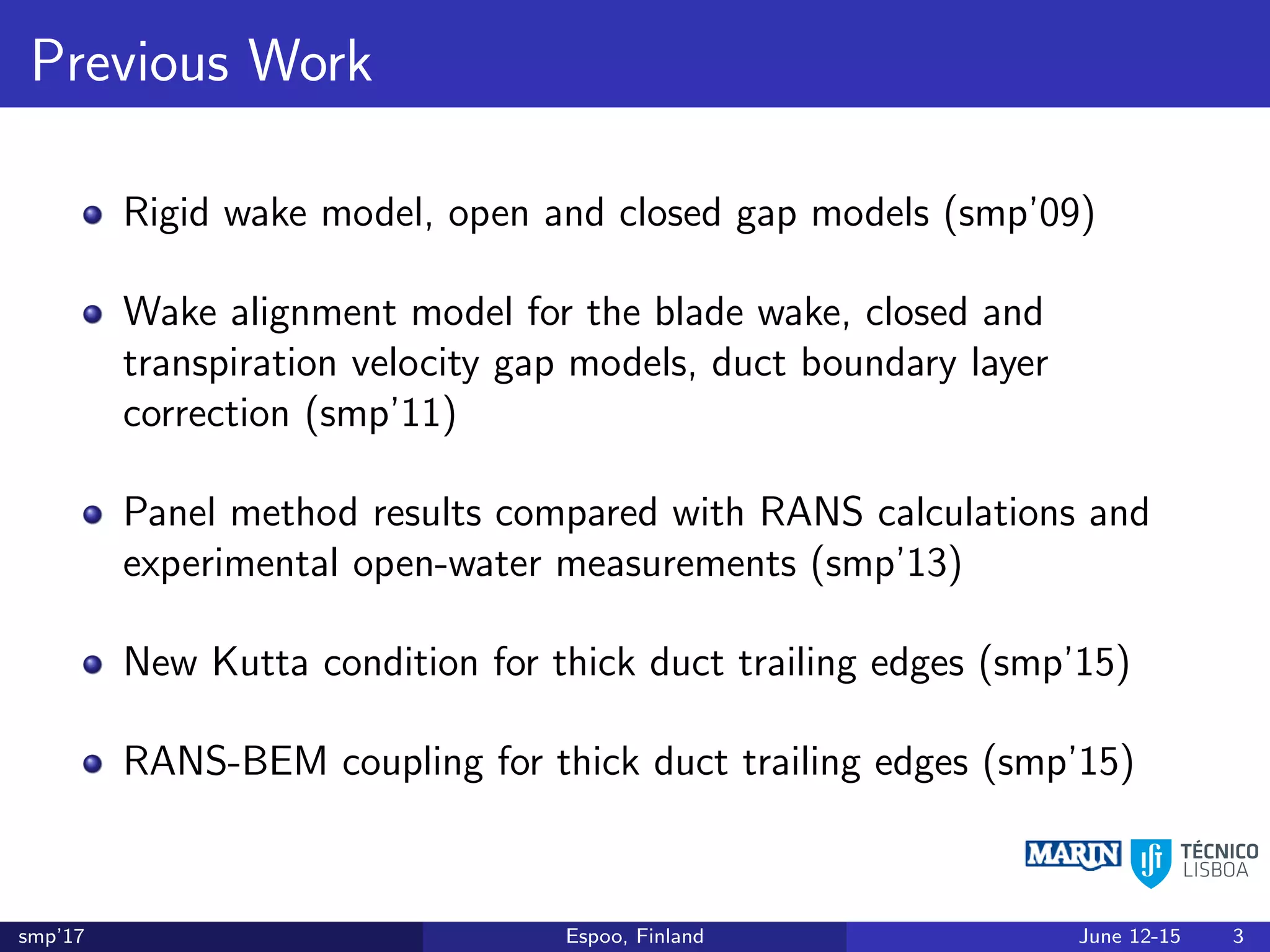
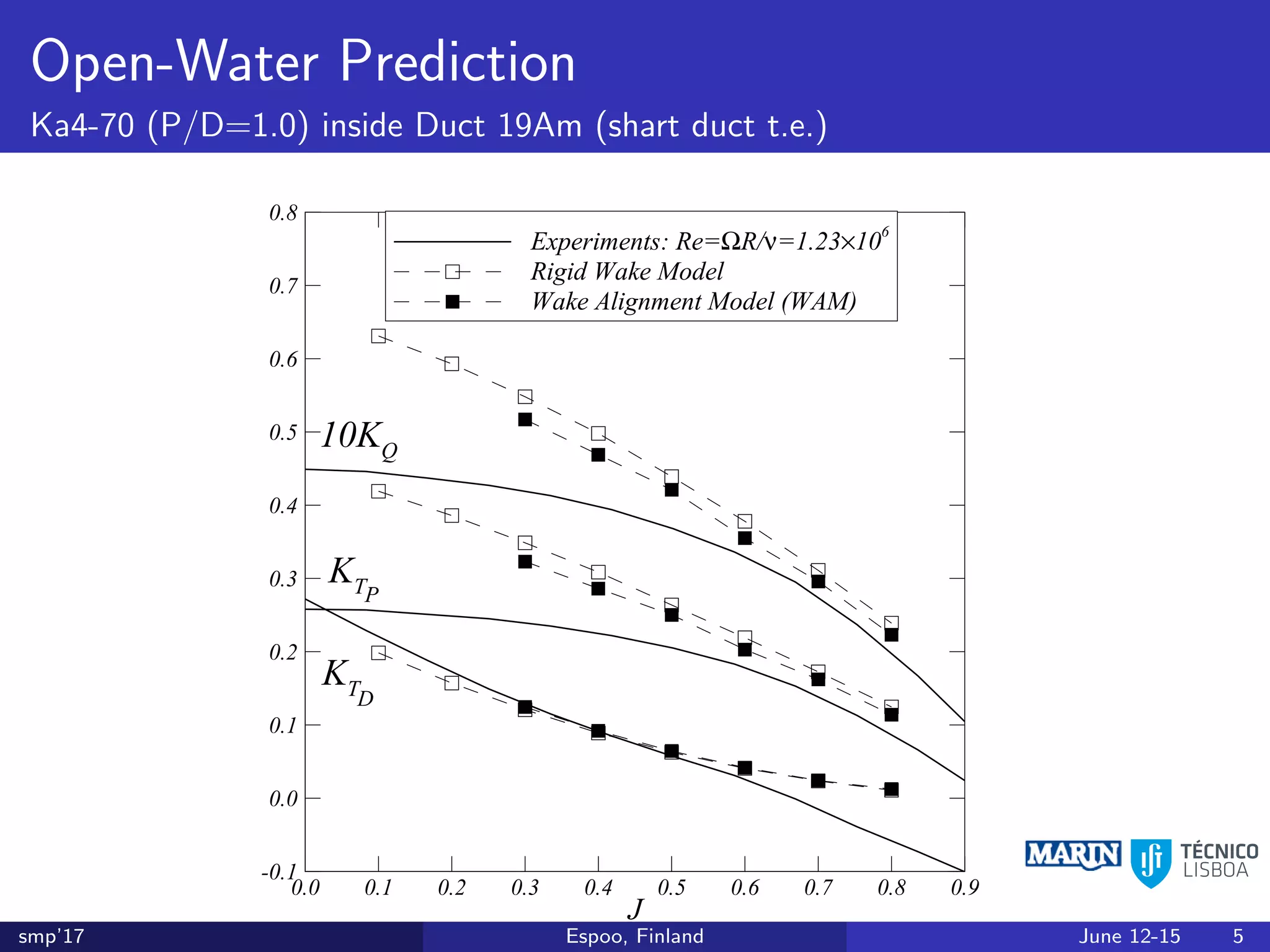
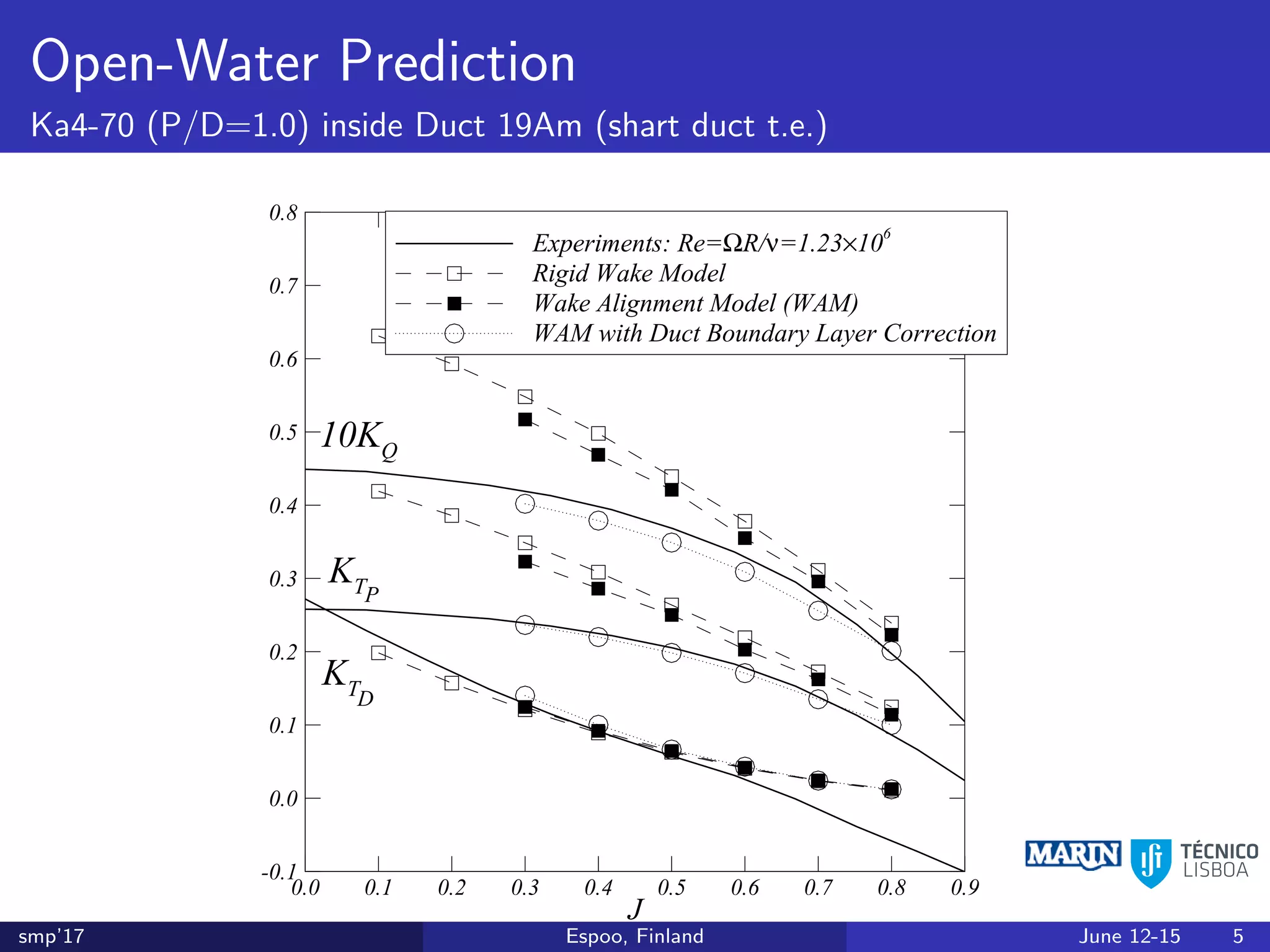
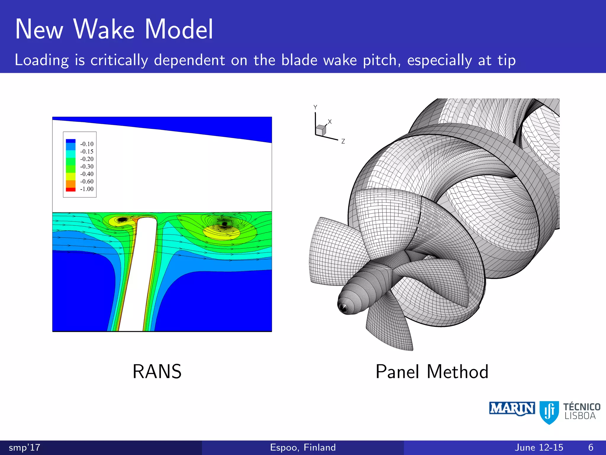
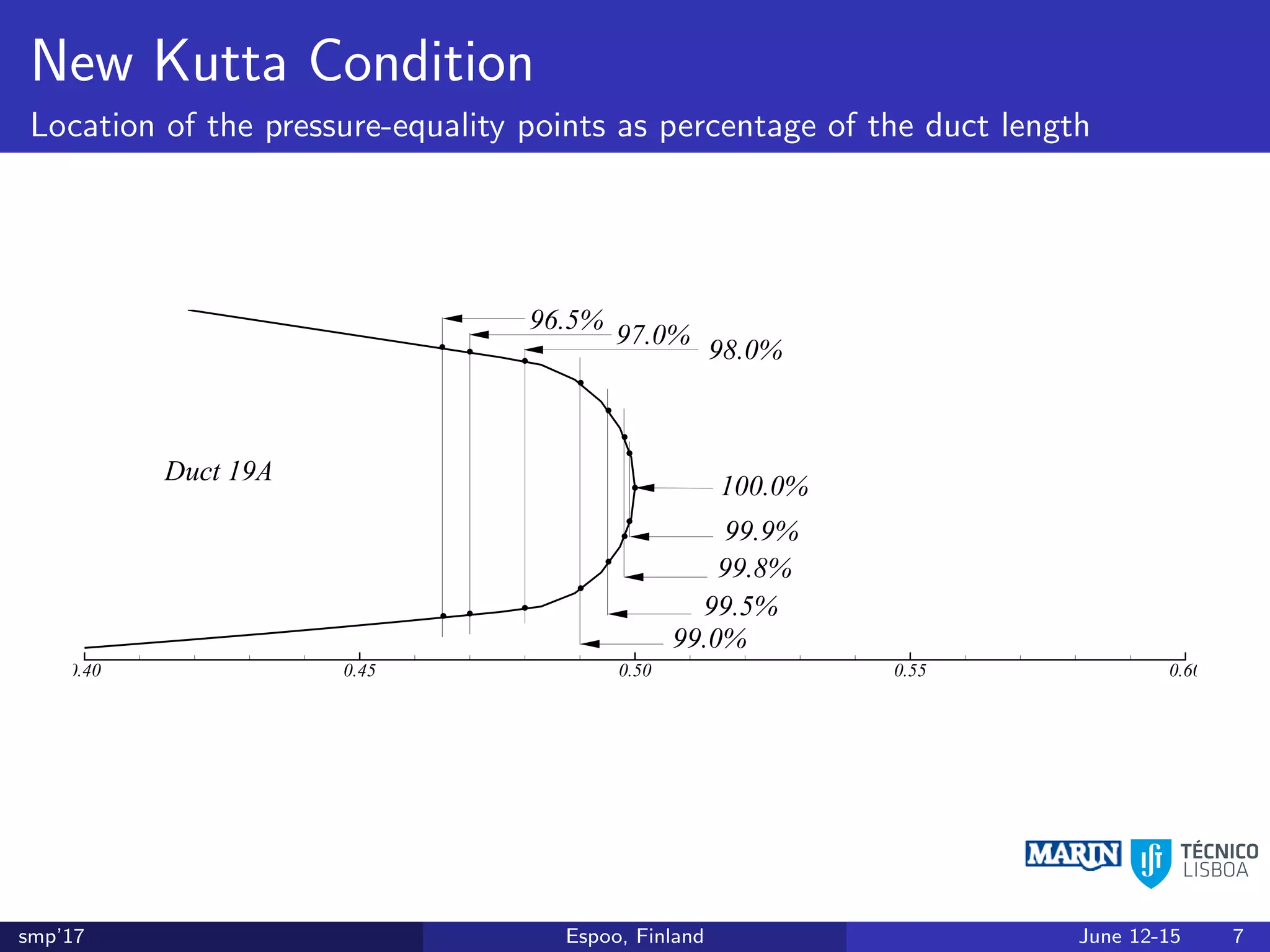
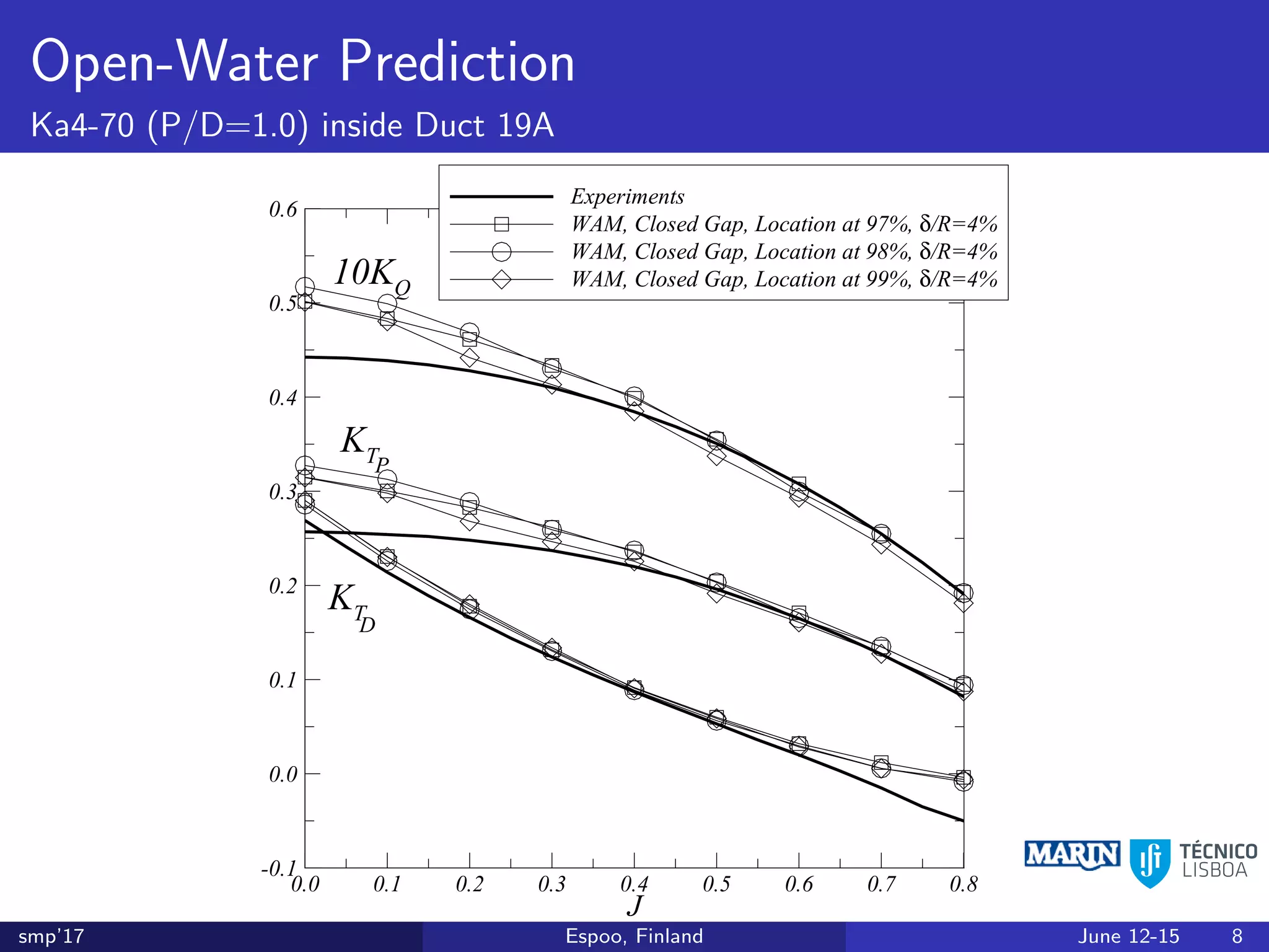
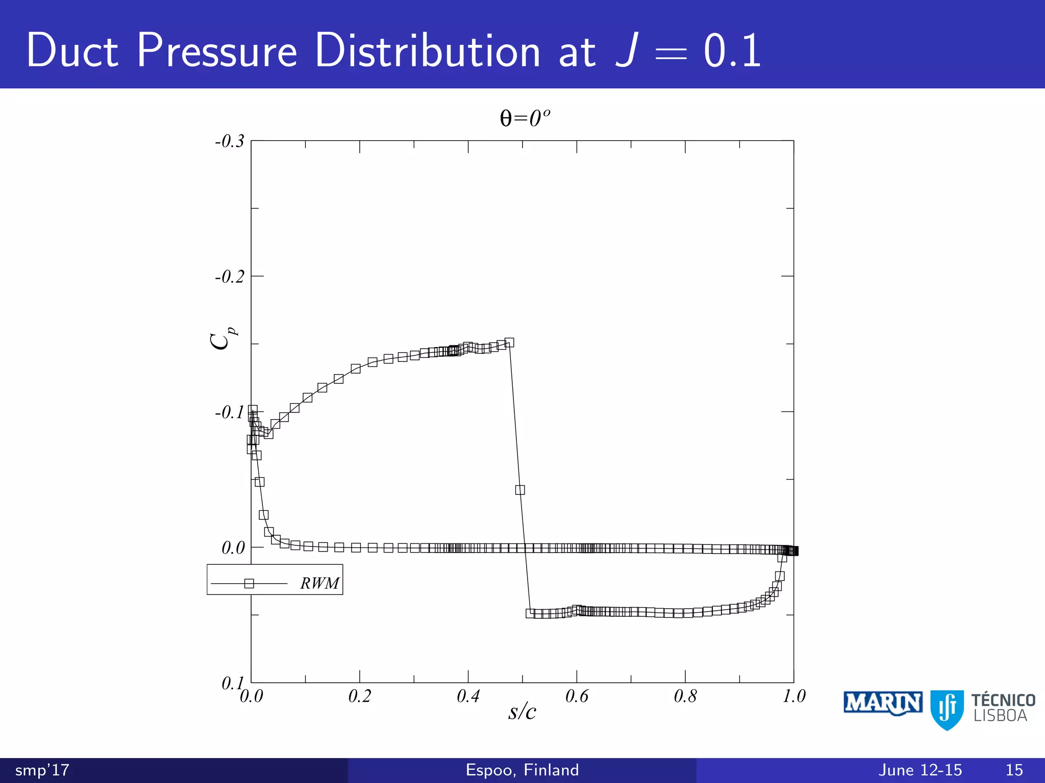
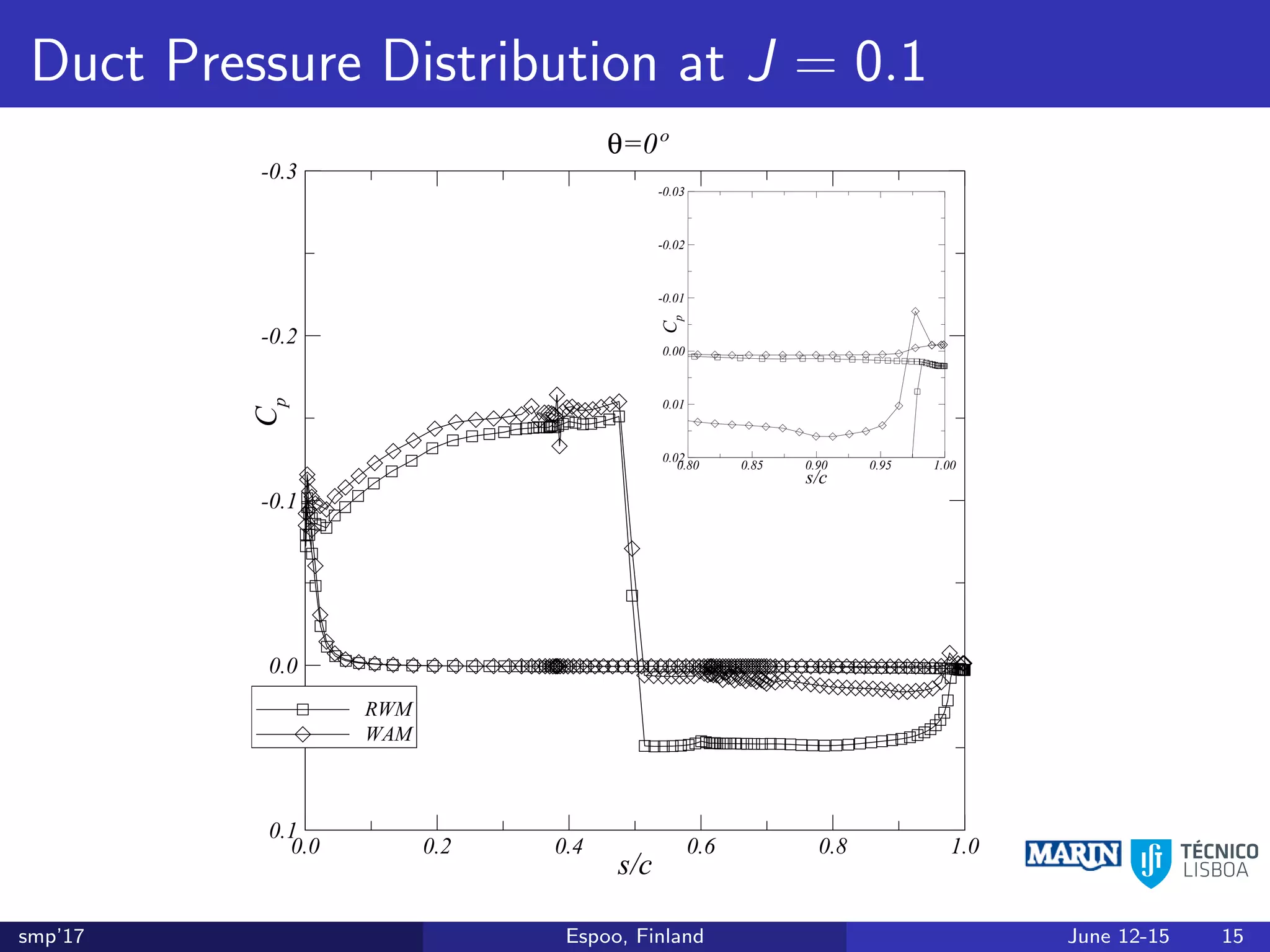
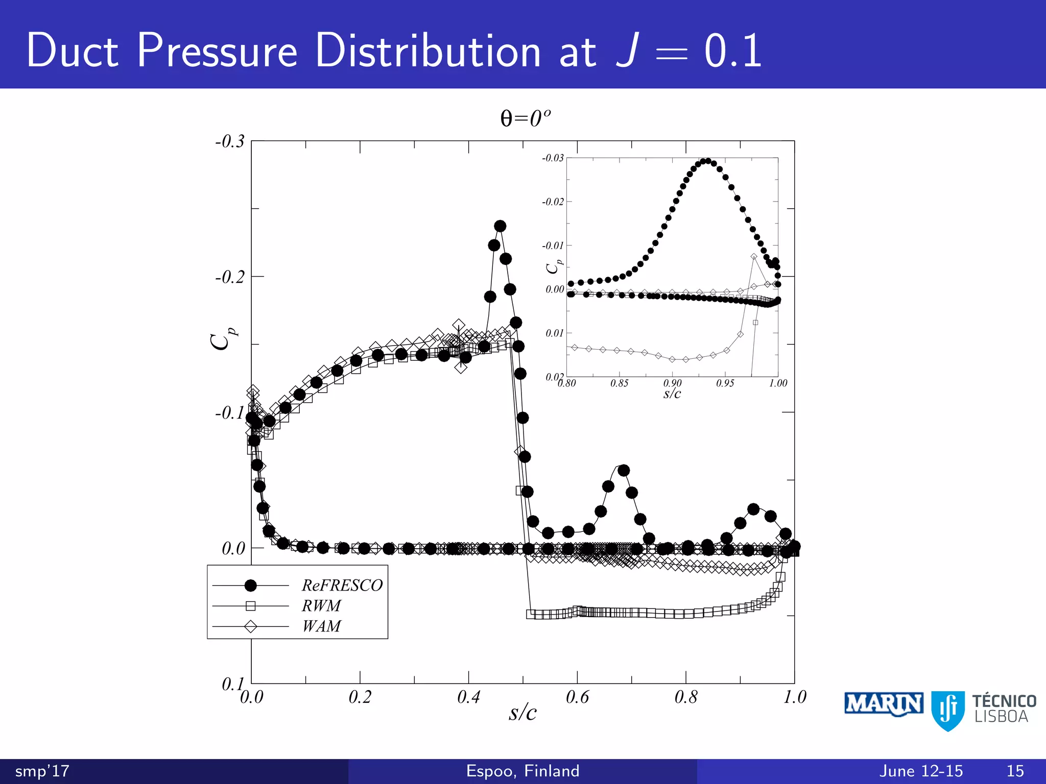
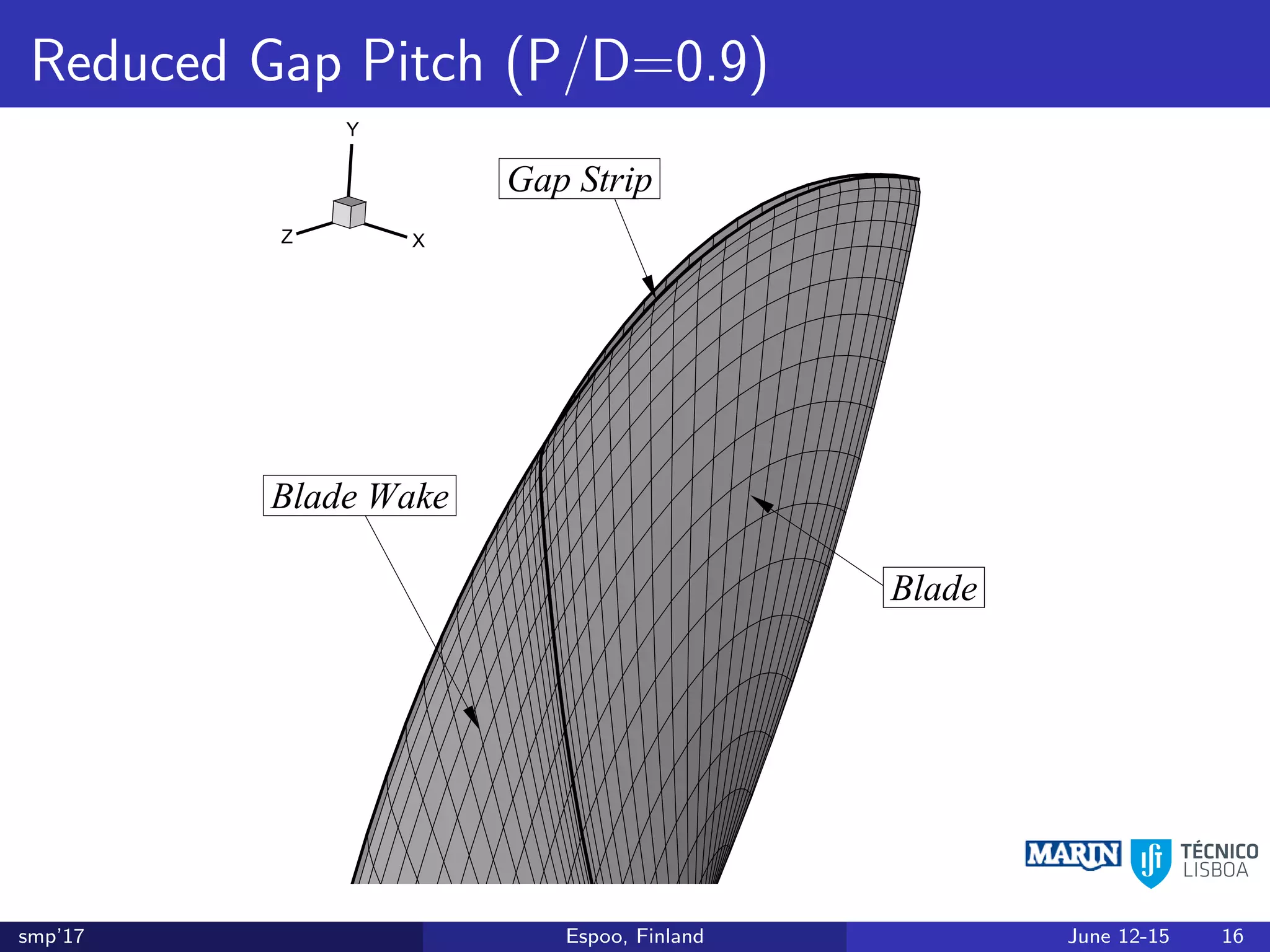
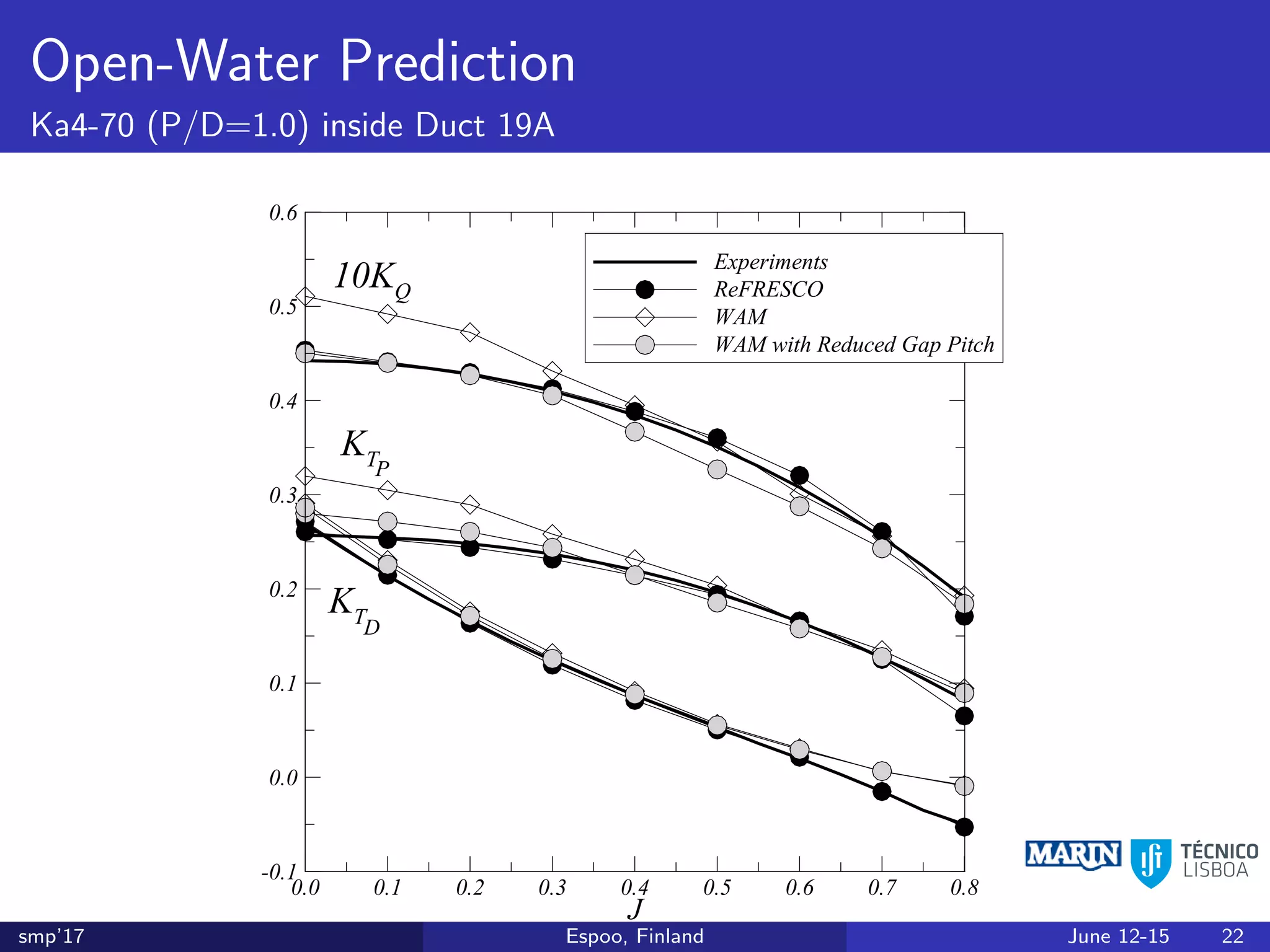
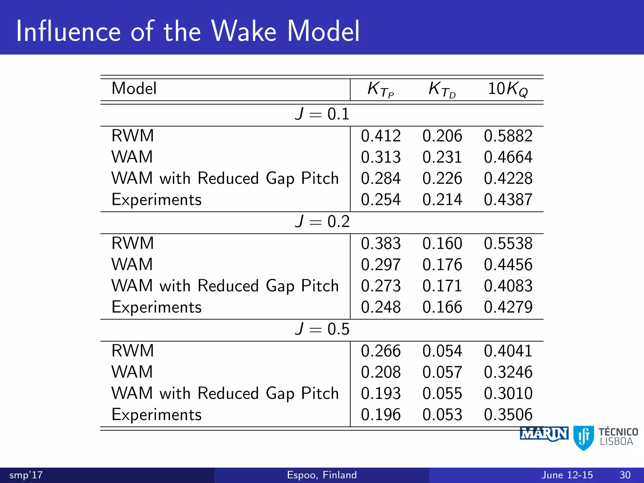
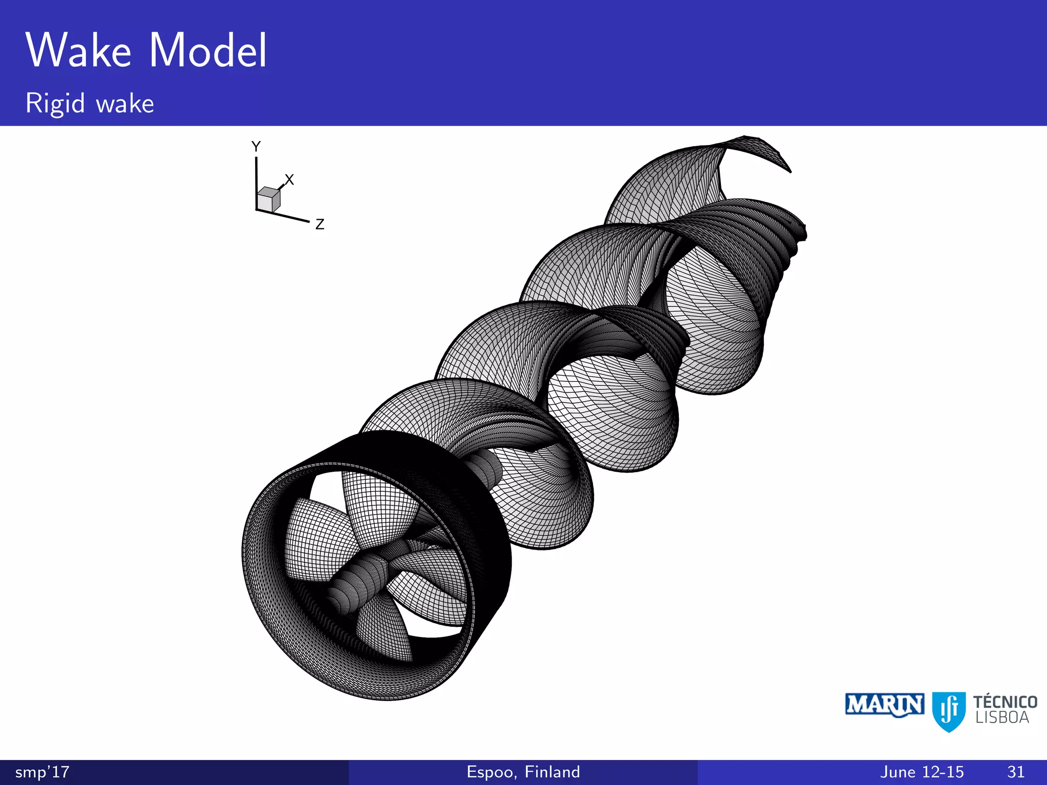
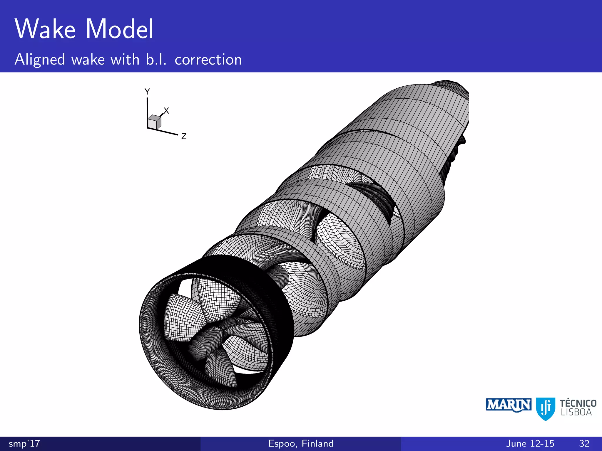
Prediction of the Open-Water Performance
of Ducted Propellers With a Panel Method
J. Baltazar1, D. Rijpkema2, J.A.C. Falc˜ao de Campos1, J. Bosschers2
1Instituto Superior T´ecnico, Universidade de Lisboa, Portugal
2Maritime Research Institute Netherlands, Wageningen, the Netherlands
smp’17 Espoo, Finland June 12-15 1
Introduction
smp’17 Espoo, Finland June 12-15 2
Introduction
Panel Methods (or BEM) still provide a most useful
computational tool for analysis and design of marine propulsors
smp’17 Espoo, Finland June 12-15 2
Introduction
Panel Methods (or BEM) still provide a most useful
computational tool for analysis and design of marine propulsors
Main reasons for using Panel Methods:
smp’17 Espoo, Finland June 12-15 2
Introduction
Panel Methods (or BEM) still provide a most useful
computational tool for analysis and design of marine propulsors
Main reasons for using Panel Methods:
Simplicity
smp’17 Espoo, Finland June 12-15 2
Introduction
Panel Methods (or BEM) still provide a most useful
computational tool for analysis and design of marine propulsors
Main reasons for using Panel Methods:
Simplicity
Computational efficiency
smp’17 Espoo, Finland June 12-15 2
Introduction
Panel Methods (or BEM) still provide a most useful
computational tool for analysis and design of marine propulsors
Main reasons for using Panel Methods:
Simplicity
Computational efficiency
Direct relation to simpler design tools
(lifting line and lifting surface)
Application to ducted propellers involves additional modelling
issues:
Complex interaction of propeller blades and duct surface
– Gap flow –
Thick duct trailing edges in practical applications
– Kutta condition for round trailing edges –
smp’17 Espoo, Finland June 12-15 2
Previous Work
smp’17 Espoo, Finland June 12-15 3
Previous Work
Rigid wake model, open and closed gap models (smp’09)
smp’17 Espoo, Finland June 12-15 3
Previous Work
Rigid wake model, open and closed gap models (smp’09)
Wake alignment model for the blade wake, closed and
transpiration velocity gap models, duct boundary layer
correction (smp’11)
smp’17 Espoo, Finland June 12-15 3
Previous Work
Rigid wake model, open and closed gap models (smp’09)
Wake alignment model for the blade wake, closed and
transpiration velocity gap models, duct boundary layer
correction (smp’11)
Panel method results compared with RANS calculations and
experimental open-water measurements (smp’13)
New Kutta condition for thick duct trailing edges (smp’15)
RANS-BEM coupling for thick duct trailing edges (smp’15)
smp’17 Espoo, Finland June 12-15 3
Duct Geometries
smp’17 Espoo, Finland June 12-15 4
Open-Water Prediction
Ka4-70 (P/D=1.0) inside Duct 19Am (shart duct t.e.)
J
0.0 0.1 0.2 0.3 0.4 0.5 0.6 0.7 0.8 0.9
-0.1
0.0
0.1
0.2
0.3
0.4
0.5
0.6
0.7
0.8
Experiments: Re=ΩR/ν=1.23×10
6
KT
10KQ
KTD
P
smp’17 Espoo, Finland June 12-15 5
Open-Water Prediction
Ka4-70 (P/D=1.0) inside Duct 19Am (shart duct t.e.)
J
0.0 0.1 0.2 0.3 0.4 0.5 0.6 0.7 0.8 0.9
-0.1
0.0
0.1
0.2
0.3
0.4
0.5
0.6
0.7
0.8
Experiments: Re=ΩR/ν=1.23×10
6
KT
10KQ
KTD
P
J
0.0 0.1 0.2 0.3 0.4 0.5 0.6 0.7 0.8 0.9
-0.1
0.0
0.1
0.2
0.3
0.4
0.5
0.6
0.7
0.8
Experiments: Re=ΩR/ν=1.23×10
6
Rigid Wake Model
KT
10KQ
KTD
P
J
0.0 0.1 0.2 0.3 0.4 0.5 0.6 0.7 0.8 0.9
-0.1
0.0
0.1
0.2
0.3
0.4
0.5
0.6
0.7
0.8
Experiments: Re=ΩR/ν=1.23×10
6
Rigid Wake Model
Wake Alignment Model (WAM)
KT
10KQ
KTD
P
J
0.0 0.1 0.2 0.3 0.4 0.5 0.6 0.7 0.8 0.9
-0.1
0.0
0.1
0.2
0.3
0.4
0.5
0.6
0.7
0.8
Experiments: Re=ΩR/ν=1.23×10
6
Rigid Wake Model
Wake Alignment Model (WAM)
WAM with Duct Boundary Layer Correction
KT
10KQ
KTD
P
smp’17 Espoo, Finland June 12-15 5
New Wake Model
Loading is critically dependent on the blade wake pitch, especially at tip
RANS Panel Method
smp’17 Espoo, Finland June 12-15 6
New Kutta Condition
Location of the pressure-equality points as percentage of the duct length
0.40 0.45 0.50 0.55 0.60
Duct 19A
100.0%
99.9%
99.8%
99.5%
99.0%
97.0%
96.5%
98.0%
smp’17 Espoo, Finland June 12-15 7
Open-Water Prediction
Ka4-70 (P/D=1.0) inside Duct 19A
J
0.0 0.1 0.2 0.3 0.4 0.5 0.6 0.7 0.8
-0.1
0.0
0.1
0.2
0.3
0.4
0.5
0.6
Experiments
WAM, Closed Gap, Location at 97%, δ/R=4%
WAM, Closed Gap, Location at 98%, δ/R=4%
WAM, Closed Gap, Location at 99%, δ/R=4%
KT
10KQ
KT
D
P
smp’17 Espoo, Finland June 12-15 8
Motivation
smp’17 Espoo, Finland June 12-15 9
Motivation
Panel Method:
smp’17 Espoo, Finland June 12-15 9
Motivation
Panel Method:
Gap model (closed)
smp’17 Espoo, Finland June 12-15 9
Motivation
Panel Method:
Gap model (closed)
Wake alignment model
smp’17 Espoo, Finland June 12-15 9
Motivation
Panel Method:
Gap model (closed)
Wake alignment model
Correction due to duct boundary layer
smp’17 Espoo, Finland June 12-15 9
Motivation
Panel Method:
Gap model (closed)
Wake alignment model
Correction due to duct boundary layer
New Kutta condition for thick duct t.e.
smp’17 Espoo, Finland June 12-15 9
Motivation
Panel Method:
Gap model (closed)
Wake alignment model
Correction due to duct boundary layer
New Kutta condition for thick duct t.e.
Significant differences in the performance prediction close to
bollard pull condition!
smp’17 Espoo, Finland June 12-15 9
Motivation
Panel Method:
Gap model (closed)
Wake alignment model
Correction due to duct boundary layer
New Kutta condition for thick duct t.e.
Significant differences in the performance prediction close to
bollard pull condition!
Comparison between Panel Method and RANS calculations
smp’17 Espoo, Finland June 12-15 9
Numerical Methods
smp’17 Espoo, Finland June 12-15 10
Numerical Methods
Panel Code PROPAN
smp’17 Espoo, Finland June 12-15 10
Numerical Methods
Panel Code PROPAN
IST in-house low-order potential-based panel method
smp’17 Espoo, Finland June 12-15 10
Numerical Methods
Panel Code PROPAN
IST in-house low-order potential-based panel method
Fredholm integral equation solved by the collocation method
smp’17 Espoo, Finland June 12-15 10
Numerical Methods
Panel Code PROPAN
IST in-house low-order potential-based panel method
Fredholm integral equation solved by the collocation method
Structured surface grids
smp’17 Espoo, Finland June 12-15 10
Numerical Methods
Panel Code PROPAN
IST in-house low-order potential-based panel method
Fredholm integral equation solved by the collocation method
Structured surface grids
RANS Code ReFRESCO
smp’17 Espoo, Finland June 12-15 10
Numerical Methods
Panel Code PROPAN
IST in-house low-order potential-based panel method
Fredholm integral equation solved by the collocation method
Structured surface grids
RANS Code ReFRESCO
Viscous flow CFD code (development led by MARIN)
smp’17 Espoo, Finland June 12-15 10
Numerical Methods
Panel Code PROPAN
IST in-house low-order potential-based panel method
Fredholm integral equation solved by the collocation method
Structured surface grids
RANS Code ReFRESCO
Viscous flow CFD code (development led by MARIN)
Finite volume discretisation
Turbulence model: k − ω SST 2-equation model
by Menter (1994)
No wal functions are used (y+ ∼ 1)
smp’17 Espoo, Finland June 12-15 10
Grids
PROPAN (left) and ReFRESCO (right)
Blade: 50×26 27M Cells
Duct: 190×160
smp’17 Espoo, Finland June 12-15 11
Blade Pressure Distribution at J = 0.5
s/c
Cp
0.0 0.2 0.4 0.6 0.8 1.0
-0.5
0.0
0.5
1.0
RWM
r/R=0.95
Cp=-1.0
smp’17 Espoo, Finland June 12-15 12
Blade Pressure Distribution at J = 0.5
s/c
Cp
0.0 0.2 0.4 0.6 0.8 1.0
-0.5
0.0
0.5
1.0
RWM
r/R=0.95
Cp=-1.0
s/c
Cp
0.0 0.2 0.4 0.6 0.8 1.0
-0.5
0.0
0.5
1.0
RWM
WAM
r/R=0.95
s/c
Cp
0.00 0.01 0.02 0.03 0.04 0.05
-0.5
0.0
0.5
1.0
smp’17 Espoo, Finland June 12-15 12
Blade Pressure Distribution at J = 0.5
s/c
Cp
0.0 0.2 0.4 0.6 0.8 1.0
-0.5
0.0
0.5
1.0
RWM
r/R=0.95
Cp=-1.0
s/c
Cp
0.0 0.2 0.4 0.6 0.8 1.0
-0.5
0.0
0.5
1.0
RWM
WAM
r/R=0.95
s/c
Cp
0.00 0.01 0.02 0.03 0.04 0.05
-0.5
0.0
0.5
1.0
s/c
Cp
0.0 0.2 0.4 0.6 0.8 1.0
-0.5
0.0
0.5
1.0
ReFRESCO
RWM
WAM
r/R=0.95
s/c
Cp
0.00 0.01 0.02 0.03 0.04 0.05
-0.5
0.0
0.5
1.0
smp’17 Espoo, Finland June 12-15 12
Duct Pressure Distribution at J = 0.5
s/c
Cp
0.0 0.2 0.4 0.6 0.8 1.0
-0.2
-0.1
0.0
0.1
RWM
θ=0º
s/c
Cp
0.80 0.85 0.90 0.95 1.00
-0.03
-0.02
-0.01
0.00
0.01
0.02
smp’17 Espoo, Finland June 12-15 13
Duct Pressure Distribution at J = 0.5
s/c
Cp
0.0 0.2 0.4 0.6 0.8 1.0
-0.2
-0.1
0.0
0.1
RWM
θ=0º
s/c
Cp
0.80 0.85 0.90 0.95 1.00
-0.03
-0.02
-0.01
0.00
0.01
0.02
s/c
Cp
0.0 0.2 0.4 0.6 0.8 1.0
-0.2
-0.1
0.0
0.1
RWM
WAM
θ=0º
s/c
Cp
0.80 0.85 0.90 0.95 1.00
-0.03
-0.02
-0.01
0.00
0.01
0.02
s/c
Cp
0.0 0.2 0.4 0.6 0.8 1.0
-0.2
-0.1
0.0
0.1
ReFRESCO
RWM
WAM
θ=0º
s/c
Cp
0.80 0.85 0.90 0.95 1.00
-0.03
-0.02
-0.01
0.00
0.01
0.02
smp’17 Espoo, Finland June 12-15 13
Blade Pressure Distribution at J = 0.1
s/c
Cp
0.0 0.2 0.4 0.6 0.8 1.0
-1.0
-0.5
0.0
0.5
RWM
r/R=0.95
Cp
=-4.0
smp’17 Espoo, Finland June 12-15 14
Blade Pressure Distribution at J = 0.1
s/c
Cp
0.0 0.2 0.4 0.6 0.8 1.0
-1.0
-0.5
0.0
0.5
RWM
r/R=0.95
Cp
=-4.0
s/c
Cp
0.0 0.2 0.4 0.6 0.8 1.0
-1.0
-0.5
0.0
0.5
RWM
WAM
r/R=0.95
s/c
Cp
0.00 0.01 0.02 0.03 0.04 0.05
-2.0
-1.5
-1.0
-0.5
0.0
0.5
1.0
smp’17 Espoo, Finland June 12-15 14
Blade Pressure Distribution at J = 0.1
s/c
Cp
0.0 0.2 0.4 0.6 0.8 1.0
-1.0
-0.5
0.0
0.5
RWM
r/R=0.95
Cp
=-4.0
s/c
Cp
0.0 0.2 0.4 0.6 0.8 1.0
-1.0
-0.5
0.0
0.5
RWM
WAM
r/R=0.95
s/c
Cp
0.00 0.01 0.02 0.03 0.04 0.05
-2.0
-1.5
-1.0
-0.5
0.0
0.5
1.0
s/c
Cp
0.0 0.2 0.4 0.6 0.8 1.0
-1.0
-0.5
0.0
0.5
ReFRESCO
RWM
WAM
r/R=0.95
s/c
Cp
0.00 0.01 0.02 0.03 0.04 0.05
-2.0
-1.5
-1.0
-0.5
0.0
0.5
1.0
smp’17 Espoo, Finland June 12-15 14
Duct Pressure Distribution at J = 0.1
s/c
Cp
0.0 0.2 0.4 0.6 0.8 1.0
-0.3
-0.2
-0.1
0.0
0.1
RWM
θ=0º
smp’17 Espoo, Finland June 12-15 15
Duct Pressure Distribution at J = 0.1
s/c
Cp
0.0 0.2 0.4 0.6 0.8 1.0
-0.3
-0.2
-0.1
0.0
0.1
RWM
θ=0º
s/c
Cp
0.0 0.2 0.4 0.6 0.8 1.0
-0.3
-0.2
-0.1
0.0
0.1
RWM
WAM
θ=0º
s/c
Cp
0.80 0.85 0.90 0.95 1.00
-0.03
-0.02
-0.01
0.00
0.01
0.02
smp’17 Espoo, Finland June 12-15 15
Duct Pressure Distribution at J = 0.1
s/c
Cp
0.0 0.2 0.4 0.6 0.8 1.0
-0.3
-0.2
-0.1
0.0
0.1
RWM
θ=0º
s/c
Cp
0.0 0.2 0.4 0.6 0.8 1.0
-0.3
-0.2
-0.1
0.0
0.1
RWM
WAM
θ=0º
s/c
Cp
0.80 0.85 0.90 0.95 1.00
-0.03
-0.02
-0.01
0.00
0.01
0.02
s/c
Cp
0.0 0.2 0.4 0.6 0.8 1.0
-0.3
-0.2
-0.1
0.0
0.1
ReFRESCO
RWM
WAM
θ=0º
s/c
Cp
0.80 0.85 0.90 0.95 1.00
-0.03
-0.02
-0.01
0.00
0.01
0.02
smp’17 Espoo, Finland June 12-15 15
Reduced Gap Pitch (P/D=0.9)
X
Y
Z
Blade
Blade Wake
Gap Strip
smp’17 Espoo, Finland June 12-15 16
Reduced Gap Pitch (P/D=0.9)
X
Y
Z
Blade
Blade Wake
Gap Strip
X
Y
Z
Blade
Blade Wake
Gap Strip
smp’17 Espoo, Finland June 12-15 16
Tip Leakage Flow
smp’17 Espoo, Finland June 12-15 17
Pressure Distribution at J = 0.5
s/c
Cp
0.0 0.2 0.4 0.6 0.8 1.0
-0.5
0.0
0.5
1.0
ReFRESCO
RWM
WAM
WAM with Reduced Gap Pitch
r/R=0.95
s/c
Cp
0.00 0.01 0.02 0.03 0.04 0.05
-0.5
0.0
0.5
1.0
smp’17 Espoo, Finland June 12-15 18
Pressure Distribution at J = 0.5
s/c
Cp
0.0 0.2 0.4 0.6 0.8 1.0
-0.2
-0.1
0.0
0.1
ReFRESCO
RWM
WAM
WAM with Reduced Gap Pitch
θ=0º
s/c
Cp
0.80 0.85 0.90 0.95 1.00
-0.03
-0.02
-0.01
0.00
0.01
0.02
smp’17 Espoo, Finland June 12-15 19
Blade Pressure Distribution at J = 0.1
s/c
Cp
0.0 0.2 0.4 0.6 0.8 1.0
-1.0
-0.5
0.0
0.5
RWM
r/R=0.95
Cp
=-4.0
smp’17 Espoo, Finland June 12-15 20
Blade Pressure Distribution at J = 0.1
s/c
Cp
0.0 0.2 0.4 0.6 0.8 1.0
-1.0
-0.5
0.0
0.5
RWM
r/R=0.95
Cp
=-4.0
s/c
Cp
0.0 0.2 0.4 0.6 0.8 1.0
-1.0
-0.5
0.0
0.5
RWM
WAM
r/R=0.95
s/c
Cp
0.00 0.01 0.02 0.03 0.04 0.05
-2.0
-1.5
-1.0
-0.5
0.0
0.5
1.0
smp’17 Espoo, Finland June 12-15 20
Blade Pressure Distribution at J = 0.1
s/c
Cp
0.0 0.2 0.4 0.6 0.8 1.0
-1.0
-0.5
0.0
0.5
RWM
r/R=0.95
Cp
=-4.0
s/c
Cp
0.0 0.2 0.4 0.6 0.8 1.0
-1.0
-0.5
0.0
0.5
RWM
WAM
r/R=0.95
s/c
Cp
0.00 0.01 0.02 0.03 0.04 0.05
-2.0
-1.5
-1.0
-0.5
0.0
0.5
1.0
s/c
Cp
0.0 0.2 0.4 0.6 0.8 1.0
-1.0
-0.5
0.0
0.5
RWM
WAM
WAM with Reduced Gap Pitch
r/R=0.95
s/c
Cp
0.00 0.01 0.02 0.03 0.04 0.05
-2.0
-1.5
-1.0
-0.5
0.0
0.5
1.0
s/c
Cp
0.0 0.2 0.4 0.6 0.8 1.0
-1.0
-0.5
0.0
0.5
ReFRESCO
RWM
WAM
WAM with Reduced Gap Pitch
r/R=0.95
s/c
Cp
0.00 0.01 0.02 0.03 0.04 0.05
-2.0
-1.5
-1.0
-0.5
0.0
0.5
1.0
smp’17 Espoo, Finland June 12-15 20
Duct Pressure Distribution at J = 0.1
s/c
Cp
0.0 0.2 0.4 0.6 0.8 1.0
-0.3
-0.2
-0.1
0.0
0.1
RWM
θ=0º
smp’17 Espoo, Finland June 12-15 21
Duct Pressure Distribution at J = 0.1
s/c
Cp
0.0 0.2 0.4 0.6 0.8 1.0
-0.3
-0.2
-0.1
0.0
0.1
RWM
θ=0º
s/c
Cp
0.0 0.2 0.4 0.6 0.8 1.0
-0.3
-0.2
-0.1
0.0
0.1
RWM
WAM
θ=0º
s/c
Cp
0.80 0.85 0.90 0.95 1.00
-0.03
-0.02
-0.01
0.00
0.01
0.02
smp’17 Espoo, Finland June 12-15 21
Duct Pressure Distribution at J = 0.1
s/c
Cp
0.0 0.2 0.4 0.6 0.8 1.0
-0.3
-0.2
-0.1
0.0
0.1
RWM
θ=0º
s/c
Cp
0.0 0.2 0.4 0.6 0.8 1.0
-0.3
-0.2
-0.1
0.0
0.1
RWM
WAM
θ=0º
s/c
Cp
0.80 0.85 0.90 0.95 1.00
-0.03
-0.02
-0.01
0.00
0.01
0.02
s/c
Cp
0.0 0.2 0.4 0.6 0.8 1.0
-0.3
-0.2
-0.1
0.0
0.1
RWM
WAM
WAM with Reduced Gap Pitch
θ=0º
s/c
Cp
0.80 0.85 0.90 0.95 1.00
-0.03
-0.02
-0.01
0.00
0.01
0.02
s/c
Cp
0.0 0.2 0.4 0.6 0.8 1.0
-0.3
-0.2
-0.1
0.0
0.1
ReFRESCO
RWM
WAM
WAM with Reduced Gap Pitch
θ=0º
s/c
Cp
0.80 0.85 0.90 0.95 1.00
-0.03
-0.02
-0.01
0.00
0.01
0.02
smp’17 Espoo, Finland June 12-15 21
Open-Water Prediction
Ka4-70 (P/D=1.0) inside Duct 19A
J
0.0 0.1 0.2 0.3 0.4 0.5 0.6 0.7 0.8
-0.1
0.0
0.1
0.2
0.3
0.4
0.5
0.6
Experiments
KT
10KQ
KT
D
P
smp’17 Espoo, Finland June 12-15 22
Open-Water Prediction
Ka4-70 (P/D=1.0) inside Duct 19A
J
0.0 0.1 0.2 0.3 0.4 0.5 0.6 0.7 0.8
-0.1
0.0
0.1
0.2
0.3
0.4
0.5
0.6
Experiments
KT
10KQ
KT
D
P
J
0.0 0.1 0.2 0.3 0.4 0.5 0.6 0.7 0.8
-0.1
0.0
0.1
0.2
0.3
0.4
0.5
0.6
Experiments
ReFRESCO
KT
10KQ
KT
D
P
smp’17 Espoo, Finland June 12-15 22
Open-Water Prediction
Ka4-70 (P/D=1.0) inside Duct 19A
J
0.0 0.1 0.2 0.3 0.4 0.5 0.6 0.7 0.8
-0.1
0.0
0.1
0.2
0.3
0.4
0.5
0.6
Experiments
KT
10KQ
KT
D
P
J
0.0 0.1 0.2 0.3 0.4 0.5 0.6 0.7 0.8
-0.1
0.0
0.1
0.2
0.3
0.4
0.5
0.6
Experiments
ReFRESCO
KT
10KQ
KT
D
P
J
0.0 0.1 0.2 0.3 0.4 0.5 0.6 0.7 0.8
-0.1
0.0
0.1
0.2
0.3
0.4
0.5
0.6
Experiments
ReFRESCO
WAM
KT
10KQ
KT
D
P
J
0.0 0.1 0.2 0.3 0.4 0.5 0.6 0.7 0.8
-0.1
0.0
0.1
0.2
0.3
0.4
0.5
0.6
Experiments
ReFRESCO
WAM
WAM with Reduced Gap Pitch
KT
10KQ
KT
D
P
smp’17 Espoo, Finland June 12-15 22
Conclusions
smp’17 Espoo, Finland June 12-15 23
Conclusions
Prediction of the ducted propeller loading is critically dependent
on the blade wake pitch, especially at tip!
smp’17 Espoo, Finland June 12-15 23
Conclusions
Prediction of the ducted propeller loading is critically dependent
on the blade wake pitch, especially at tip!
The flow in the tip region is particularly important near
bollard pull
smp’17 Espoo, Finland June 12-15 23
Conclusions
Prediction of the ducted propeller loading is critically dependent
on the blade wake pitch, especially at tip!
The flow in the tip region is particularly important near
bollard pull
Future work:
smp’17 Espoo, Finland June 12-15 23
Conclusions
Prediction of the ducted propeller loading is critically dependent
on the blade wake pitch, especially at tip!
The flow in the tip region is particularly important near
bollard pull
Future work:
Include reduction of the gap strip in wake alignment model
Robustness issues are expected
smp’17 Espoo, Finland June 12-15 23
Pressure Distribution at J = 0.2
s/c
Cp
0.0 0.2 0.4 0.6 0.8 1.0
-1.0
-0.5
0.0
0.5
ReFRESCO
RWM
WAM
WAM with Reduced Gap Pitch
r/R=0.95
s/c
Cp
0.00 0.01 0.02 0.03 0.04 0.05
-2.0
-1.5
-1.0
-0.5
0.0
0.5
1.0
s/c
Cp
0.0 0.2 0.4 0.6 0.8 1.0
-0.3
-0.2
-0.1
0.0
0.1
ReFRESCO
RWM
WAM
WAM with Reduced Gap Pitch
θ=0º
s/c
Cp
0.80 0.85 0.90 0.95 1.00
-0.03
-0.02
-0.01
0.00
0.01
0.02
smp’17 Espoo, Finland June 12-15 24
Wake Geometry at J = 0.2
x/R = 0.2 x/R = 0.4
smp’17 Espoo, Finland June 12-15 25
Wake Geometry at J = 0.2
smp’17 Espoo, Finland June 12-15 26
Wake Geometry at J = 0.1
x/R = 0.2 x/R = 0.4
smp’17 Espoo, Finland June 12-15 27
Wake Geometry at J = 0.1
smp’17 Espoo, Finland June 12-15 28
Wake Geometry at J = 0.5
x/R = 0.2 x/R = 0.4
smp’17 Espoo, Finland June 12-15 29
Influence of the Wake Model
Model KTP
KTD
10KQ
J = 0.1
RWM 0.412 0.206 0.5882
WAM 0.313 0.231 0.4664
WAM with Reduced Gap Pitch 0.284 0.226 0.4228
Experiments 0.254 0.214 0.4387
J = 0.2
RWM 0.383 0.160 0.5538
WAM 0.297 0.176 0.4456
WAM with Reduced Gap Pitch 0.273 0.171 0.4083
Experiments 0.248 0.166 0.4279
J = 0.5
RWM 0.266 0.054 0.4041
WAM 0.208 0.057 0.3246
WAM with Reduced Gap Pitch 0.193 0.055 0.3010
Experiments 0.196 0.053 0.3506
smp’17 Espoo, Finland June 12-15 30
Wake Model
Rigid wake
X
Y
Z
smp’17 Espoo, Finland June 12-15 31
Wake Model
Aligned wake with b.l. correction
X
Y
Z
smp’17 Espoo, Finland June 12-15 32

Prediction of the Open-Water Performance of Ducted Propellers With a Panel Method

  • 1.
    Prediction of theOpen-Water Performance of Ducted Propellers With a Panel Method J. Baltazar1, D. Rijpkema2, J.A.C. Falc˜ao de Campos1, J. Bosschers2 1Instituto Superior T´ecnico, Universidade de Lisboa, Portugal 2Maritime Research Institute Netherlands, Wageningen, the Netherlands smp’17 Espoo, Finland June 12-15 1
  • 2.
  • 3.
    Introduction Panel Methods (orBEM) still provide a most useful computational tool for analysis and design of marine propulsors smp’17 Espoo, Finland June 12-15 2
  • 4.
    Introduction Panel Methods (orBEM) still provide a most useful computational tool for analysis and design of marine propulsors Main reasons for using Panel Methods: smp’17 Espoo, Finland June 12-15 2
  • 5.
    Introduction Panel Methods (orBEM) still provide a most useful computational tool for analysis and design of marine propulsors Main reasons for using Panel Methods: Simplicity smp’17 Espoo, Finland June 12-15 2
  • 6.
    Introduction Panel Methods (orBEM) still provide a most useful computational tool for analysis and design of marine propulsors Main reasons for using Panel Methods: Simplicity Computational efficiency smp’17 Espoo, Finland June 12-15 2
  • 7.
    Introduction Panel Methods (orBEM) still provide a most useful computational tool for analysis and design of marine propulsors Main reasons for using Panel Methods: Simplicity Computational efficiency Direct relation to simpler design tools (lifting line and lifting surface) smp’17 Espoo, Finland June 12-15 2
  • 8.
    Introduction Panel Methods (orBEM) still provide a most useful computational tool for analysis and design of marine propulsors Main reasons for using Panel Methods: Simplicity Computational efficiency Direct relation to simpler design tools (lifting line and lifting surface) Application to ducted propellers involves additional modelling issues: smp’17 Espoo, Finland June 12-15 2
  • 9.
    Introduction Panel Methods (orBEM) still provide a most useful computational tool for analysis and design of marine propulsors Main reasons for using Panel Methods: Simplicity Computational efficiency Direct relation to simpler design tools (lifting line and lifting surface) Application to ducted propellers involves additional modelling issues: Complex interaction of propeller blades and duct surface – Gap flow – smp’17 Espoo, Finland June 12-15 2
  • 10.
    Introduction Panel Methods (orBEM) still provide a most useful computational tool for analysis and design of marine propulsors Main reasons for using Panel Methods: Simplicity Computational efficiency Direct relation to simpler design tools (lifting line and lifting surface) Application to ducted propellers involves additional modelling issues: Complex interaction of propeller blades and duct surface – Gap flow – Thick duct trailing edges in practical applications – Kutta condition for round trailing edges – smp’17 Espoo, Finland June 12-15 2
  • 11.
    Introduction Panel Methods (orBEM) still provide a most useful computational tool for analysis and design of marine propulsors Main reasons for using Panel Methods: Simplicity Computational efficiency Direct relation to simpler design tools (lifting line and lifting surface) Application to ducted propellers involves additional modelling issues: Complex interaction of propeller blades and duct surface – Gap flow – Thick duct trailing edges in practical applications – Kutta condition for round trailing edges – smp’17 Espoo, Finland June 12-15 2
  • 12.
    Previous Work smp’17 Espoo,Finland June 12-15 3
  • 13.
    Previous Work Rigid wakemodel, open and closed gap models (smp’09) smp’17 Espoo, Finland June 12-15 3
  • 14.
    Previous Work Rigid wakemodel, open and closed gap models (smp’09) Wake alignment model for the blade wake, closed and transpiration velocity gap models, duct boundary layer correction (smp’11) smp’17 Espoo, Finland June 12-15 3
  • 15.
    Previous Work Rigid wakemodel, open and closed gap models (smp’09) Wake alignment model for the blade wake, closed and transpiration velocity gap models, duct boundary layer correction (smp’11) Panel method results compared with RANS calculations and experimental open-water measurements (smp’13) smp’17 Espoo, Finland June 12-15 3
  • 16.
    Previous Work Rigid wakemodel, open and closed gap models (smp’09) Wake alignment model for the blade wake, closed and transpiration velocity gap models, duct boundary layer correction (smp’11) Panel method results compared with RANS calculations and experimental open-water measurements (smp’13) New Kutta condition for thick duct trailing edges (smp’15) smp’17 Espoo, Finland June 12-15 3
  • 17.
    Previous Work Rigid wakemodel, open and closed gap models (smp’09) Wake alignment model for the blade wake, closed and transpiration velocity gap models, duct boundary layer correction (smp’11) Panel method results compared with RANS calculations and experimental open-water measurements (smp’13) New Kutta condition for thick duct trailing edges (smp’15) RANS-BEM coupling for thick duct trailing edges (smp’15) smp’17 Espoo, Finland June 12-15 3
  • 18.
    Duct Geometries smp’17 Espoo,Finland June 12-15 4
  • 19.
    Open-Water Prediction Ka4-70 (P/D=1.0)inside Duct 19Am (shart duct t.e.) J 0.0 0.1 0.2 0.3 0.4 0.5 0.6 0.7 0.8 0.9 -0.1 0.0 0.1 0.2 0.3 0.4 0.5 0.6 0.7 0.8 Experiments: Re=ΩR/ν=1.23×10 6 KT 10KQ KTD P smp’17 Espoo, Finland June 12-15 5
  • 20.
    Open-Water Prediction Ka4-70 (P/D=1.0)inside Duct 19Am (shart duct t.e.) J 0.0 0.1 0.2 0.3 0.4 0.5 0.6 0.7 0.8 0.9 -0.1 0.0 0.1 0.2 0.3 0.4 0.5 0.6 0.7 0.8 Experiments: Re=ΩR/ν=1.23×10 6 KT 10KQ KTD P J 0.0 0.1 0.2 0.3 0.4 0.5 0.6 0.7 0.8 0.9 -0.1 0.0 0.1 0.2 0.3 0.4 0.5 0.6 0.7 0.8 Experiments: Re=ΩR/ν=1.23×10 6 Rigid Wake Model KT 10KQ KTD P smp’17 Espoo, Finland June 12-15 5
  • 21.
    Open-Water Prediction Ka4-70 (P/D=1.0)inside Duct 19Am (shart duct t.e.) J 0.0 0.1 0.2 0.3 0.4 0.5 0.6 0.7 0.8 0.9 -0.1 0.0 0.1 0.2 0.3 0.4 0.5 0.6 0.7 0.8 Experiments: Re=ΩR/ν=1.23×10 6 KT 10KQ KTD P J 0.0 0.1 0.2 0.3 0.4 0.5 0.6 0.7 0.8 0.9 -0.1 0.0 0.1 0.2 0.3 0.4 0.5 0.6 0.7 0.8 Experiments: Re=ΩR/ν=1.23×10 6 Rigid Wake Model KT 10KQ KTD P J 0.0 0.1 0.2 0.3 0.4 0.5 0.6 0.7 0.8 0.9 -0.1 0.0 0.1 0.2 0.3 0.4 0.5 0.6 0.7 0.8 Experiments: Re=ΩR/ν=1.23×10 6 Rigid Wake Model Wake Alignment Model (WAM) KT 10KQ KTD P smp’17 Espoo, Finland June 12-15 5
  • 22.
    Open-Water Prediction Ka4-70 (P/D=1.0)inside Duct 19Am (shart duct t.e.) J 0.0 0.1 0.2 0.3 0.4 0.5 0.6 0.7 0.8 0.9 -0.1 0.0 0.1 0.2 0.3 0.4 0.5 0.6 0.7 0.8 Experiments: Re=ΩR/ν=1.23×10 6 KT 10KQ KTD P J 0.0 0.1 0.2 0.3 0.4 0.5 0.6 0.7 0.8 0.9 -0.1 0.0 0.1 0.2 0.3 0.4 0.5 0.6 0.7 0.8 Experiments: Re=ΩR/ν=1.23×10 6 Rigid Wake Model KT 10KQ KTD P J 0.0 0.1 0.2 0.3 0.4 0.5 0.6 0.7 0.8 0.9 -0.1 0.0 0.1 0.2 0.3 0.4 0.5 0.6 0.7 0.8 Experiments: Re=ΩR/ν=1.23×10 6 Rigid Wake Model Wake Alignment Model (WAM) KT 10KQ KTD P J 0.0 0.1 0.2 0.3 0.4 0.5 0.6 0.7 0.8 0.9 -0.1 0.0 0.1 0.2 0.3 0.4 0.5 0.6 0.7 0.8 Experiments: Re=ΩR/ν=1.23×10 6 Rigid Wake Model Wake Alignment Model (WAM) WAM with Duct Boundary Layer Correction KT 10KQ KTD P smp’17 Espoo, Finland June 12-15 5
  • 23.
    New Wake Model Loadingis critically dependent on the blade wake pitch, especially at tip RANS Panel Method smp’17 Espoo, Finland June 12-15 6
  • 24.
    New Kutta Condition Locationof the pressure-equality points as percentage of the duct length 0.40 0.45 0.50 0.55 0.60 Duct 19A 100.0% 99.9% 99.8% 99.5% 99.0% 97.0% 96.5% 98.0% smp’17 Espoo, Finland June 12-15 7
  • 25.
    Open-Water Prediction Ka4-70 (P/D=1.0)inside Duct 19A J 0.0 0.1 0.2 0.3 0.4 0.5 0.6 0.7 0.8 -0.1 0.0 0.1 0.2 0.3 0.4 0.5 0.6 Experiments WAM, Closed Gap, Location at 97%, δ/R=4% WAM, Closed Gap, Location at 98%, δ/R=4% WAM, Closed Gap, Location at 99%, δ/R=4% KT 10KQ KT D P smp’17 Espoo, Finland June 12-15 8
  • 26.
  • 27.
  • 28.
    Motivation Panel Method: Gap model(closed) smp’17 Espoo, Finland June 12-15 9
  • 29.
    Motivation Panel Method: Gap model(closed) Wake alignment model smp’17 Espoo, Finland June 12-15 9
  • 30.
    Motivation Panel Method: Gap model(closed) Wake alignment model Correction due to duct boundary layer smp’17 Espoo, Finland June 12-15 9
  • 31.
    Motivation Panel Method: Gap model(closed) Wake alignment model Correction due to duct boundary layer New Kutta condition for thick duct t.e. smp’17 Espoo, Finland June 12-15 9
  • 32.
    Motivation Panel Method: Gap model(closed) Wake alignment model Correction due to duct boundary layer New Kutta condition for thick duct t.e. Significant differences in the performance prediction close to bollard pull condition! smp’17 Espoo, Finland June 12-15 9
  • 33.
    Motivation Panel Method: Gap model(closed) Wake alignment model Correction due to duct boundary layer New Kutta condition for thick duct t.e. Significant differences in the performance prediction close to bollard pull condition! Comparison between Panel Method and RANS calculations smp’17 Espoo, Finland June 12-15 9
  • 34.
    Motivation Panel Method: Gap model(closed) Wake alignment model Correction due to duct boundary layer New Kutta condition for thick duct t.e. Significant differences in the performance prediction close to bollard pull condition! Comparison between Panel Method and RANS calculations smp’17 Espoo, Finland June 12-15 9
  • 35.
    Numerical Methods smp’17 Espoo,Finland June 12-15 10
  • 36.
    Numerical Methods Panel CodePROPAN smp’17 Espoo, Finland June 12-15 10
  • 37.
    Numerical Methods Panel CodePROPAN IST in-house low-order potential-based panel method smp’17 Espoo, Finland June 12-15 10
  • 38.
    Numerical Methods Panel CodePROPAN IST in-house low-order potential-based panel method Fredholm integral equation solved by the collocation method smp’17 Espoo, Finland June 12-15 10
  • 39.
    Numerical Methods Panel CodePROPAN IST in-house low-order potential-based panel method Fredholm integral equation solved by the collocation method Structured surface grids smp’17 Espoo, Finland June 12-15 10
  • 40.
    Numerical Methods Panel CodePROPAN IST in-house low-order potential-based panel method Fredholm integral equation solved by the collocation method Structured surface grids RANS Code ReFRESCO smp’17 Espoo, Finland June 12-15 10
  • 41.
    Numerical Methods Panel CodePROPAN IST in-house low-order potential-based panel method Fredholm integral equation solved by the collocation method Structured surface grids RANS Code ReFRESCO Viscous flow CFD code (development led by MARIN) smp’17 Espoo, Finland June 12-15 10
  • 42.
    Numerical Methods Panel CodePROPAN IST in-house low-order potential-based panel method Fredholm integral equation solved by the collocation method Structured surface grids RANS Code ReFRESCO Viscous flow CFD code (development led by MARIN) Finite volume discretisation smp’17 Espoo, Finland June 12-15 10
  • 43.
    Numerical Methods Panel CodePROPAN IST in-house low-order potential-based panel method Fredholm integral equation solved by the collocation method Structured surface grids RANS Code ReFRESCO Viscous flow CFD code (development led by MARIN) Finite volume discretisation Turbulence model: k − ω SST 2-equation model by Menter (1994) smp’17 Espoo, Finland June 12-15 10
  • 44.
    Numerical Methods Panel CodePROPAN IST in-house low-order potential-based panel method Fredholm integral equation solved by the collocation method Structured surface grids RANS Code ReFRESCO Viscous flow CFD code (development led by MARIN) Finite volume discretisation Turbulence model: k − ω SST 2-equation model by Menter (1994) No wal functions are used (y+ ∼ 1) smp’17 Espoo, Finland June 12-15 10
  • 45.
    Grids PROPAN (left) andReFRESCO (right) Blade: 50×26 27M Cells Duct: 190×160 smp’17 Espoo, Finland June 12-15 11
  • 46.
    Blade Pressure Distributionat J = 0.5 s/c Cp 0.0 0.2 0.4 0.6 0.8 1.0 -0.5 0.0 0.5 1.0 RWM r/R=0.95 Cp=-1.0 smp’17 Espoo, Finland June 12-15 12
  • 47.
    Blade Pressure Distributionat J = 0.5 s/c Cp 0.0 0.2 0.4 0.6 0.8 1.0 -0.5 0.0 0.5 1.0 RWM r/R=0.95 Cp=-1.0 s/c Cp 0.0 0.2 0.4 0.6 0.8 1.0 -0.5 0.0 0.5 1.0 RWM WAM r/R=0.95 s/c Cp 0.00 0.01 0.02 0.03 0.04 0.05 -0.5 0.0 0.5 1.0 smp’17 Espoo, Finland June 12-15 12
  • 48.
    Blade Pressure Distributionat J = 0.5 s/c Cp 0.0 0.2 0.4 0.6 0.8 1.0 -0.5 0.0 0.5 1.0 RWM r/R=0.95 Cp=-1.0 s/c Cp 0.0 0.2 0.4 0.6 0.8 1.0 -0.5 0.0 0.5 1.0 RWM WAM r/R=0.95 s/c Cp 0.00 0.01 0.02 0.03 0.04 0.05 -0.5 0.0 0.5 1.0 s/c Cp 0.0 0.2 0.4 0.6 0.8 1.0 -0.5 0.0 0.5 1.0 ReFRESCO RWM WAM r/R=0.95 s/c Cp 0.00 0.01 0.02 0.03 0.04 0.05 -0.5 0.0 0.5 1.0 smp’17 Espoo, Finland June 12-15 12
  • 49.
    Duct Pressure Distributionat J = 0.5 s/c Cp 0.0 0.2 0.4 0.6 0.8 1.0 -0.2 -0.1 0.0 0.1 RWM θ=0º s/c Cp 0.80 0.85 0.90 0.95 1.00 -0.03 -0.02 -0.01 0.00 0.01 0.02 smp’17 Espoo, Finland June 12-15 13
  • 50.
    Duct Pressure Distributionat J = 0.5 s/c Cp 0.0 0.2 0.4 0.6 0.8 1.0 -0.2 -0.1 0.0 0.1 RWM θ=0º s/c Cp 0.80 0.85 0.90 0.95 1.00 -0.03 -0.02 -0.01 0.00 0.01 0.02 s/c Cp 0.0 0.2 0.4 0.6 0.8 1.0 -0.2 -0.1 0.0 0.1 RWM WAM θ=0º s/c Cp 0.80 0.85 0.90 0.95 1.00 -0.03 -0.02 -0.01 0.00 0.01 0.02 smp’17 Espoo, Finland June 12-15 13
  • 51.
    Duct Pressure Distributionat J = 0.5 s/c Cp 0.0 0.2 0.4 0.6 0.8 1.0 -0.2 -0.1 0.0 0.1 RWM θ=0º s/c Cp 0.80 0.85 0.90 0.95 1.00 -0.03 -0.02 -0.01 0.00 0.01 0.02 s/c Cp 0.0 0.2 0.4 0.6 0.8 1.0 -0.2 -0.1 0.0 0.1 RWM WAM θ=0º s/c Cp 0.80 0.85 0.90 0.95 1.00 -0.03 -0.02 -0.01 0.00 0.01 0.02 s/c Cp 0.0 0.2 0.4 0.6 0.8 1.0 -0.2 -0.1 0.0 0.1 ReFRESCO RWM WAM θ=0º s/c Cp 0.80 0.85 0.90 0.95 1.00 -0.03 -0.02 -0.01 0.00 0.01 0.02 smp’17 Espoo, Finland June 12-15 13
  • 52.
    Blade Pressure Distributionat J = 0.1 s/c Cp 0.0 0.2 0.4 0.6 0.8 1.0 -1.0 -0.5 0.0 0.5 RWM r/R=0.95 Cp =-4.0 smp’17 Espoo, Finland June 12-15 14
  • 53.
    Blade Pressure Distributionat J = 0.1 s/c Cp 0.0 0.2 0.4 0.6 0.8 1.0 -1.0 -0.5 0.0 0.5 RWM r/R=0.95 Cp =-4.0 s/c Cp 0.0 0.2 0.4 0.6 0.8 1.0 -1.0 -0.5 0.0 0.5 RWM WAM r/R=0.95 s/c Cp 0.00 0.01 0.02 0.03 0.04 0.05 -2.0 -1.5 -1.0 -0.5 0.0 0.5 1.0 smp’17 Espoo, Finland June 12-15 14
  • 54.
    Blade Pressure Distributionat J = 0.1 s/c Cp 0.0 0.2 0.4 0.6 0.8 1.0 -1.0 -0.5 0.0 0.5 RWM r/R=0.95 Cp =-4.0 s/c Cp 0.0 0.2 0.4 0.6 0.8 1.0 -1.0 -0.5 0.0 0.5 RWM WAM r/R=0.95 s/c Cp 0.00 0.01 0.02 0.03 0.04 0.05 -2.0 -1.5 -1.0 -0.5 0.0 0.5 1.0 s/c Cp 0.0 0.2 0.4 0.6 0.8 1.0 -1.0 -0.5 0.0 0.5 ReFRESCO RWM WAM r/R=0.95 s/c Cp 0.00 0.01 0.02 0.03 0.04 0.05 -2.0 -1.5 -1.0 -0.5 0.0 0.5 1.0 smp’17 Espoo, Finland June 12-15 14
  • 55.
    Duct Pressure Distributionat J = 0.1 s/c Cp 0.0 0.2 0.4 0.6 0.8 1.0 -0.3 -0.2 -0.1 0.0 0.1 RWM θ=0º smp’17 Espoo, Finland June 12-15 15
  • 56.
    Duct Pressure Distributionat J = 0.1 s/c Cp 0.0 0.2 0.4 0.6 0.8 1.0 -0.3 -0.2 -0.1 0.0 0.1 RWM θ=0º s/c Cp 0.0 0.2 0.4 0.6 0.8 1.0 -0.3 -0.2 -0.1 0.0 0.1 RWM WAM θ=0º s/c Cp 0.80 0.85 0.90 0.95 1.00 -0.03 -0.02 -0.01 0.00 0.01 0.02 smp’17 Espoo, Finland June 12-15 15
  • 57.
    Duct Pressure Distributionat J = 0.1 s/c Cp 0.0 0.2 0.4 0.6 0.8 1.0 -0.3 -0.2 -0.1 0.0 0.1 RWM θ=0º s/c Cp 0.0 0.2 0.4 0.6 0.8 1.0 -0.3 -0.2 -0.1 0.0 0.1 RWM WAM θ=0º s/c Cp 0.80 0.85 0.90 0.95 1.00 -0.03 -0.02 -0.01 0.00 0.01 0.02 s/c Cp 0.0 0.2 0.4 0.6 0.8 1.0 -0.3 -0.2 -0.1 0.0 0.1 ReFRESCO RWM WAM θ=0º s/c Cp 0.80 0.85 0.90 0.95 1.00 -0.03 -0.02 -0.01 0.00 0.01 0.02 smp’17 Espoo, Finland June 12-15 15
  • 58.
    Reduced Gap Pitch(P/D=0.9) X Y Z Blade Blade Wake Gap Strip smp’17 Espoo, Finland June 12-15 16
  • 59.
    Reduced Gap Pitch(P/D=0.9) X Y Z Blade Blade Wake Gap Strip X Y Z Blade Blade Wake Gap Strip smp’17 Espoo, Finland June 12-15 16
  • 60.
    Tip Leakage Flow smp’17Espoo, Finland June 12-15 17
  • 61.
    Pressure Distribution atJ = 0.5 s/c Cp 0.0 0.2 0.4 0.6 0.8 1.0 -0.5 0.0 0.5 1.0 ReFRESCO RWM WAM WAM with Reduced Gap Pitch r/R=0.95 s/c Cp 0.00 0.01 0.02 0.03 0.04 0.05 -0.5 0.0 0.5 1.0 smp’17 Espoo, Finland June 12-15 18
  • 62.
    Pressure Distribution atJ = 0.5 s/c Cp 0.0 0.2 0.4 0.6 0.8 1.0 -0.2 -0.1 0.0 0.1 ReFRESCO RWM WAM WAM with Reduced Gap Pitch θ=0º s/c Cp 0.80 0.85 0.90 0.95 1.00 -0.03 -0.02 -0.01 0.00 0.01 0.02 smp’17 Espoo, Finland June 12-15 19
  • 63.
    Blade Pressure Distributionat J = 0.1 s/c Cp 0.0 0.2 0.4 0.6 0.8 1.0 -1.0 -0.5 0.0 0.5 RWM r/R=0.95 Cp =-4.0 smp’17 Espoo, Finland June 12-15 20
  • 64.
    Blade Pressure Distributionat J = 0.1 s/c Cp 0.0 0.2 0.4 0.6 0.8 1.0 -1.0 -0.5 0.0 0.5 RWM r/R=0.95 Cp =-4.0 s/c Cp 0.0 0.2 0.4 0.6 0.8 1.0 -1.0 -0.5 0.0 0.5 RWM WAM r/R=0.95 s/c Cp 0.00 0.01 0.02 0.03 0.04 0.05 -2.0 -1.5 -1.0 -0.5 0.0 0.5 1.0 smp’17 Espoo, Finland June 12-15 20
  • 65.
    Blade Pressure Distributionat J = 0.1 s/c Cp 0.0 0.2 0.4 0.6 0.8 1.0 -1.0 -0.5 0.0 0.5 RWM r/R=0.95 Cp =-4.0 s/c Cp 0.0 0.2 0.4 0.6 0.8 1.0 -1.0 -0.5 0.0 0.5 RWM WAM r/R=0.95 s/c Cp 0.00 0.01 0.02 0.03 0.04 0.05 -2.0 -1.5 -1.0 -0.5 0.0 0.5 1.0 s/c Cp 0.0 0.2 0.4 0.6 0.8 1.0 -1.0 -0.5 0.0 0.5 RWM WAM WAM with Reduced Gap Pitch r/R=0.95 s/c Cp 0.00 0.01 0.02 0.03 0.04 0.05 -2.0 -1.5 -1.0 -0.5 0.0 0.5 1.0 smp’17 Espoo, Finland June 12-15 20
  • 66.
    Blade Pressure Distributionat J = 0.1 s/c Cp 0.0 0.2 0.4 0.6 0.8 1.0 -1.0 -0.5 0.0 0.5 RWM r/R=0.95 Cp =-4.0 s/c Cp 0.0 0.2 0.4 0.6 0.8 1.0 -1.0 -0.5 0.0 0.5 RWM WAM r/R=0.95 s/c Cp 0.00 0.01 0.02 0.03 0.04 0.05 -2.0 -1.5 -1.0 -0.5 0.0 0.5 1.0 s/c Cp 0.0 0.2 0.4 0.6 0.8 1.0 -1.0 -0.5 0.0 0.5 RWM WAM WAM with Reduced Gap Pitch r/R=0.95 s/c Cp 0.00 0.01 0.02 0.03 0.04 0.05 -2.0 -1.5 -1.0 -0.5 0.0 0.5 1.0 s/c Cp 0.0 0.2 0.4 0.6 0.8 1.0 -1.0 -0.5 0.0 0.5 ReFRESCO RWM WAM WAM with Reduced Gap Pitch r/R=0.95 s/c Cp 0.00 0.01 0.02 0.03 0.04 0.05 -2.0 -1.5 -1.0 -0.5 0.0 0.5 1.0 smp’17 Espoo, Finland June 12-15 20
  • 67.
    Duct Pressure Distributionat J = 0.1 s/c Cp 0.0 0.2 0.4 0.6 0.8 1.0 -0.3 -0.2 -0.1 0.0 0.1 RWM θ=0º smp’17 Espoo, Finland June 12-15 21
  • 68.
    Duct Pressure Distributionat J = 0.1 s/c Cp 0.0 0.2 0.4 0.6 0.8 1.0 -0.3 -0.2 -0.1 0.0 0.1 RWM θ=0º s/c Cp 0.0 0.2 0.4 0.6 0.8 1.0 -0.3 -0.2 -0.1 0.0 0.1 RWM WAM θ=0º s/c Cp 0.80 0.85 0.90 0.95 1.00 -0.03 -0.02 -0.01 0.00 0.01 0.02 smp’17 Espoo, Finland June 12-15 21
  • 69.
    Duct Pressure Distributionat J = 0.1 s/c Cp 0.0 0.2 0.4 0.6 0.8 1.0 -0.3 -0.2 -0.1 0.0 0.1 RWM θ=0º s/c Cp 0.0 0.2 0.4 0.6 0.8 1.0 -0.3 -0.2 -0.1 0.0 0.1 RWM WAM θ=0º s/c Cp 0.80 0.85 0.90 0.95 1.00 -0.03 -0.02 -0.01 0.00 0.01 0.02 s/c Cp 0.0 0.2 0.4 0.6 0.8 1.0 -0.3 -0.2 -0.1 0.0 0.1 RWM WAM WAM with Reduced Gap Pitch θ=0º s/c Cp 0.80 0.85 0.90 0.95 1.00 -0.03 -0.02 -0.01 0.00 0.01 0.02 smp’17 Espoo, Finland June 12-15 21
  • 70.
    Duct Pressure Distributionat J = 0.1 s/c Cp 0.0 0.2 0.4 0.6 0.8 1.0 -0.3 -0.2 -0.1 0.0 0.1 RWM θ=0º s/c Cp 0.0 0.2 0.4 0.6 0.8 1.0 -0.3 -0.2 -0.1 0.0 0.1 RWM WAM θ=0º s/c Cp 0.80 0.85 0.90 0.95 1.00 -0.03 -0.02 -0.01 0.00 0.01 0.02 s/c Cp 0.0 0.2 0.4 0.6 0.8 1.0 -0.3 -0.2 -0.1 0.0 0.1 RWM WAM WAM with Reduced Gap Pitch θ=0º s/c Cp 0.80 0.85 0.90 0.95 1.00 -0.03 -0.02 -0.01 0.00 0.01 0.02 s/c Cp 0.0 0.2 0.4 0.6 0.8 1.0 -0.3 -0.2 -0.1 0.0 0.1 ReFRESCO RWM WAM WAM with Reduced Gap Pitch θ=0º s/c Cp 0.80 0.85 0.90 0.95 1.00 -0.03 -0.02 -0.01 0.00 0.01 0.02 smp’17 Espoo, Finland June 12-15 21
  • 71.
    Open-Water Prediction Ka4-70 (P/D=1.0)inside Duct 19A J 0.0 0.1 0.2 0.3 0.4 0.5 0.6 0.7 0.8 -0.1 0.0 0.1 0.2 0.3 0.4 0.5 0.6 Experiments KT 10KQ KT D P smp’17 Espoo, Finland June 12-15 22
  • 72.
    Open-Water Prediction Ka4-70 (P/D=1.0)inside Duct 19A J 0.0 0.1 0.2 0.3 0.4 0.5 0.6 0.7 0.8 -0.1 0.0 0.1 0.2 0.3 0.4 0.5 0.6 Experiments KT 10KQ KT D P J 0.0 0.1 0.2 0.3 0.4 0.5 0.6 0.7 0.8 -0.1 0.0 0.1 0.2 0.3 0.4 0.5 0.6 Experiments ReFRESCO KT 10KQ KT D P smp’17 Espoo, Finland June 12-15 22
  • 73.
    Open-Water Prediction Ka4-70 (P/D=1.0)inside Duct 19A J 0.0 0.1 0.2 0.3 0.4 0.5 0.6 0.7 0.8 -0.1 0.0 0.1 0.2 0.3 0.4 0.5 0.6 Experiments KT 10KQ KT D P J 0.0 0.1 0.2 0.3 0.4 0.5 0.6 0.7 0.8 -0.1 0.0 0.1 0.2 0.3 0.4 0.5 0.6 Experiments ReFRESCO KT 10KQ KT D P J 0.0 0.1 0.2 0.3 0.4 0.5 0.6 0.7 0.8 -0.1 0.0 0.1 0.2 0.3 0.4 0.5 0.6 Experiments ReFRESCO WAM KT 10KQ KT D P smp’17 Espoo, Finland June 12-15 22
  • 74.
    Open-Water Prediction Ka4-70 (P/D=1.0)inside Duct 19A J 0.0 0.1 0.2 0.3 0.4 0.5 0.6 0.7 0.8 -0.1 0.0 0.1 0.2 0.3 0.4 0.5 0.6 Experiments KT 10KQ KT D P J 0.0 0.1 0.2 0.3 0.4 0.5 0.6 0.7 0.8 -0.1 0.0 0.1 0.2 0.3 0.4 0.5 0.6 Experiments ReFRESCO KT 10KQ KT D P J 0.0 0.1 0.2 0.3 0.4 0.5 0.6 0.7 0.8 -0.1 0.0 0.1 0.2 0.3 0.4 0.5 0.6 Experiments ReFRESCO WAM KT 10KQ KT D P J 0.0 0.1 0.2 0.3 0.4 0.5 0.6 0.7 0.8 -0.1 0.0 0.1 0.2 0.3 0.4 0.5 0.6 Experiments ReFRESCO WAM WAM with Reduced Gap Pitch KT 10KQ KT D P smp’17 Espoo, Finland June 12-15 22
  • 75.
  • 76.
    Conclusions Prediction of theducted propeller loading is critically dependent on the blade wake pitch, especially at tip! smp’17 Espoo, Finland June 12-15 23
  • 77.
    Conclusions Prediction of theducted propeller loading is critically dependent on the blade wake pitch, especially at tip! The flow in the tip region is particularly important near bollard pull smp’17 Espoo, Finland June 12-15 23
  • 78.
    Conclusions Prediction of theducted propeller loading is critically dependent on the blade wake pitch, especially at tip! The flow in the tip region is particularly important near bollard pull Future work: smp’17 Espoo, Finland June 12-15 23
  • 79.
    Conclusions Prediction of theducted propeller loading is critically dependent on the blade wake pitch, especially at tip! The flow in the tip region is particularly important near bollard pull Future work: Include reduction of the gap strip in wake alignment model smp’17 Espoo, Finland June 12-15 23
  • 80.
    Conclusions Prediction of theducted propeller loading is critically dependent on the blade wake pitch, especially at tip! The flow in the tip region is particularly important near bollard pull Future work: Include reduction of the gap strip in wake alignment model Robustness issues are expected smp’17 Espoo, Finland June 12-15 23
  • 81.
    Pressure Distribution atJ = 0.2 s/c Cp 0.0 0.2 0.4 0.6 0.8 1.0 -1.0 -0.5 0.0 0.5 ReFRESCO RWM WAM WAM with Reduced Gap Pitch r/R=0.95 s/c Cp 0.00 0.01 0.02 0.03 0.04 0.05 -2.0 -1.5 -1.0 -0.5 0.0 0.5 1.0 s/c Cp 0.0 0.2 0.4 0.6 0.8 1.0 -0.3 -0.2 -0.1 0.0 0.1 ReFRESCO RWM WAM WAM with Reduced Gap Pitch θ=0º s/c Cp 0.80 0.85 0.90 0.95 1.00 -0.03 -0.02 -0.01 0.00 0.01 0.02 smp’17 Espoo, Finland June 12-15 24
  • 82.
    Wake Geometry atJ = 0.2 x/R = 0.2 x/R = 0.4 smp’17 Espoo, Finland June 12-15 25
  • 83.
    Wake Geometry atJ = 0.2 smp’17 Espoo, Finland June 12-15 26
  • 84.
    Wake Geometry atJ = 0.1 x/R = 0.2 x/R = 0.4 smp’17 Espoo, Finland June 12-15 27
  • 85.
    Wake Geometry atJ = 0.1 smp’17 Espoo, Finland June 12-15 28
  • 86.
    Wake Geometry atJ = 0.5 x/R = 0.2 x/R = 0.4 smp’17 Espoo, Finland June 12-15 29
  • 87.
    Influence of theWake Model Model KTP KTD 10KQ J = 0.1 RWM 0.412 0.206 0.5882 WAM 0.313 0.231 0.4664 WAM with Reduced Gap Pitch 0.284 0.226 0.4228 Experiments 0.254 0.214 0.4387 J = 0.2 RWM 0.383 0.160 0.5538 WAM 0.297 0.176 0.4456 WAM with Reduced Gap Pitch 0.273 0.171 0.4083 Experiments 0.248 0.166 0.4279 J = 0.5 RWM 0.266 0.054 0.4041 WAM 0.208 0.057 0.3246 WAM with Reduced Gap Pitch 0.193 0.055 0.3010 Experiments 0.196 0.053 0.3506 smp’17 Espoo, Finland June 12-15 30
  • 88.
    Wake Model Rigid wake X Y Z smp’17Espoo, Finland June 12-15 31
  • 89.
    Wake Model Aligned wakewith b.l. correction X Y Z smp’17 Espoo, Finland June 12-15 32