Pendahuluan termo

1. Copyright © McGraw-Hill Education. Permission
required for reproduction or display.
Chapter 1
INTRODUCTION
AND BASIC
CONCEPTS
Thermodynamics:
An Engineering Approach
9th Edition
Yunus A. Cengel, Michael A. Boles,
Mehmet Kanoglu
McGraw-Hill Education, 2019

2. 2
Objectives
• Identify the unique vocabulary associated with
thermodynamics through the precise definition of basic
concepts to form a sound foundation for the development of
the principles of thermodynamics.
• Review the metric SI and the English unit systems.
• Explain the basic concepts of thermodynamics such as
system, state, state postulate, equilibrium, process, and
cycle.
• Discuss properties of a system and define density, specific
gravity, and specific weight.
• Review concepts of temperature, temperature scales,
pressure, and absolute and gage pressure.
• Introduce an intuitive systematic problem-solving technique.

3. 3
THERMODYNAMICS AND ENERGY
Thermodynamics: The science of energy.
Energy: The ability to cause changes.
The name thermodynamics stems from the
Greek words therme (heat) and dynamis
(power).
Conservation of energy principle: During
an interaction, energy can change from one
form to another but the total amount of
energy remains constant.
Energy cannot be created or destroyed.
The first law of thermodynamics: An
expression of the conservation of energy
principle.
The first law asserts that energy is a
thermodynamic property.
FIGURE 1–1
Energy cannot be created or
destroyed; it can only change
forms (the first law).

4. 4
The second law of thermodynamics: It
asserts that energy has quality as well as
quantity, and actual processes occur in the
direction of decreasing quality of energy.
Classical thermodynamics: A
macroscopic approach to the study of
thermodynamics that does not require a
knowledge of the behavior of individual
particles.
It provides a direct and easy way to the
solution of engineering problems and it is
used in this text.
Statistical thermodynamics: A
microscopic approach, based on the
average behavior of large groups of
individual particles.
FIGURE 1–2
Conservation of energy
principle for the human body.
FIGURE 1–3
Heat flows in the direction of
decreasing temperature.

5. 5
Application Areas of Thermodynamics
All activities in nature involve some interaction between
energy and matter; thus, it is hard to imagine an area that
does not relate to thermodynamics in some manner.
FIGURE 1–4
The design of many engineering
systems, such as this solar hot water
system, involves thermodynamics.

6. 6
FIGURE 1–5
Some application areas of thermodynamics.

7. 7
IMPORTANCE OF DIMENSIONS AND UNITS
Any physical quantity can be characterized by dimensions.
The magnitudes assigned to the dimensions are called units.
Some basic dimensions such as mass m, length L, time t, and
temperature T are selected as primary or fundamental
dimensions, while others such as velocity V, energy E, and volume
V are expressed in terms of the primary dimensions and are called
secondary dimensions, or derived dimensions.
Metric SI system: A simple and logical system based on a decimal
relationship between the various units.
English system: It has no apparent systematic numerical base, and
various units in this system are related to each other rather
arbitrarily.

8. 8

9. 9
Some SI and
English Units
Work = Force  Distance
1 J = 1 N∙m
1 cal = 4.1868 J
1 Btu = 1.0551 kJ
FIGURE 1–6
The SI unit prefixes are used in
all branches of engineering.
FIGURE 1–7
The definition of the force units.

10. 10
W weight
m mass
g gravitational
acceleration
FIGURE 1–8
The relative magnitudes of the
force units newton (N), kilogram-
force (kgf), and pound-force (lbf).
FIGURE 1–9
A body weighing 150 lbf on
earth will weigh only 25 lbf on
the moon.

11. 11
FIGURE 1–10
The weight of a unit mass at sea level.
FIGURE 1–11
A typical match yields about one Btu
(or one kJ) of energy if completely
burned.

12. 12
Unity Conversion Ratios
All nonprimary units (secondary units) can be
formed by combinations of primary units.
They can also be expressed more conveniently
as unity conversion ratios as
Unity conversion ratios are identically equal to 1 and are
unitless, and thus such ratios (or their inverses) can be inserted
conveniently into any calculation to properly convert units.
Dimensional homogeneity
All equations must be dimensionally homogeneous.

13. 13
FIGURE 1–14
Always check the units in your
calculations.
FIGURE 1–15
Every unity conversion ratio (as well as
its inverse) is exactly equal to 1. Shown
here are a few commonly used unity
conversion ratios, each within its own set
of parentheses.

14. 14
FIGURE 1–17
A quirk in the metric
system of units.
FIGURE 1–16
A mass of 1 lbm weighs 1 lbf on earth.

15. 15
SYSTEMS AND CONTROL VOLUMES
System: A quantity of matter or a region in space chosen for study.
Surroundings: The mass or region outside the system
Boundary: The real or imaginary surface that separates the system
from its surroundings.
The boundary of a system can be fixed or movable.
Systems may be considered to be closed or open.
Closed system (Control mass): A fixed amount of mass, and no
mass can cross its boundary.
Open system (control volume): A properly selected region in space.
It usually encloses a device that involves mass flow such as a
compressor, turbine, or nozzle. Both mass and energy can cross the
boundary of a control volume.
Control surface: The boundaries of a control volume. It can be real
or imaginary.

16. 16
FIGURE 1–20
A closed system with a moving
boundary.
FIGURE 1–19
Mass cannot cross the boundaries of
a closed system, but energy can.
FIGURE 1–18
System, surroundings, and boundary.

17. 17
FIGURE 1–21
A control volume can involve fixed, moving,
real, and imaginary boundaries.

18. 18
FIGURE 1–22
An open system (a control volume)
with one inlet and one exit.

19. 19
PROPERTIES OF A SYSTEM
Property: Any characteristic of a system.
Some familiar properties are pressure P,
temperature T, volume V, and mass m.
Properties are considered to be either
intensive or extensive.
Intensive properties: Those that are
independent of the mass of a system, such
as temperature, pressure, and density.
Extensive properties: Those whose
values depend on the size—or extent—of
the system.
Specific properties: Extensive properties
per unit mass.
FIGURE 1–23
Criterion to differentiate
intensive and extensive
properties.

20. 20
DENSITY AND SPECIFIC GRAVITY
Density
Specific volume
FIGURE 1–25
Density is mass per unit volume;
specific volume is volume
per unit mass.

21. 21
Specific gravity: The ratio of the
density of a substance to the
density of some standard substance
at a specified temperature (usually
water at 4°C).
Specific weight: The weight of
a unit volume of a substance.

22. 22
STATE AND EQUILIBRIUM
Thermodynamics deals with equilibrium states.
Equilibrium: A state of balance.
In an equilibrium state there are no unbalanced potentials (or driving
forces) within the system.
Thermal equilibrium: If the temperature is the same throughout the
entire system.
Mechanical equilibrium: If there is no change in pressure at any
point of the system with time.
Phase equilibrium: If a system involves two phases and when the
mass of each phase reaches an equilibrium level and stays there.
Chemical equilibrium: If the chemical composition of a system does
not change with time, that is, no chemical reactions occur.

23. 23
FIGURE 1–26
A system at two different states.
FIGURE 1–27
A closed system reaching thermal
equilibrium.

24. 24
PROCESSES AND CYCLES
Process: Any change that a
system undergoes from one
equilibrium state to another.
Path: The series of states through
which a system passes during a
process.
To describe a process completely,
one should specify the initial and
final states, as well as the path it
follows, and the interactions with
the surroundings. FIGURE 1–29
A process between states 1 and 2 and
the process path.

25. 25
Quasistatic or quasi-
equilibrium process: When
a process proceeds in such a
manner that the system
remains infinitesimally close
to an equilibrium state at all
times.
FIGURE 1–30
Quasi-equilibrium and nonquasi-
equilibrium compression processes.

26. 26
Process diagrams plotted by employing
thermodynamic properties as coordinates
are very useful in visualizing the
processes.
Some common properties that are used
as coordinates are temperature T,
pressure P, and volume V (or specific
volume v).
The prefix iso- is often used to designate
a process for which a particular property
remains constant.
Isothermal process: A process during
which the temperature T remains
constant.
Isobaric process: A process during
which the pressure P remains constant.
Isochoric (or isometric) process: A
process during which the specific volume
v remains constant.
Cycle: A process during which the initial
and final states are identical.
FIGURE 1–31
The P-V diagram of a compression
process.

27. 27
The Steady-Flow Process
The term steady implies no change
with time. The opposite of steady is
unsteady, or transient.
A large number of engineering
devices operate for long periods of
time under the same conditions, and
they are classified as steady-flow
devices.
Steady-flow process: A process
during which a fluid flows through a
control volume steadily.
Steady-flow conditions can be closely
approximated by devices that are
intended for continuous operation
such as turbines, pumps, boilers,
condensers, and heat exchangers or
power plants or refrigeration systems.
FIGURE 1–32
During a steady-flow process, fluid
properties within the control volume
may change with position but not with time.

28. 28
FIGURE 1–33
Under steady-flow conditions, the
mass and energy contents of a control
volume remain constant.

29. 29
TEMPERATURE AND THE ZEROTH
LAW OF THERMODYNAMICS
The zeroth law of
thermodynamics: If two bodies
are in thermal equilibrium with a
third body, they are also in
thermal equilibrium with each
other.
By replacing the third body with
a thermometer, the zeroth law
can be restated as two bodies
are in thermal equilibrium if both
have the same temperature
reading even if they are not in
contact.
FIGURE 1–34
Two bodies reaching thermal
equilibrium after being brought into
contact in an isolated enclosure.

30. 30
Temperature Scales
All temperature scales are based on some easily reproducible states
such as the freezing and boiling points of water: the ice point and the
steam point.
Ice point: A mixture of ice and water that is in equilibrium with air
saturated with vapor at 1 atm pressure (0°C or 32°F).
Steam point: A mixture of liquid water and water vapor (with no air)
in equilibrium at 1 atm pressure (100°C or 212°F).
Celsius scale: Temperature in SI unit system
Fahrenheit scale: Temperature in English unit system
Thermodynamic temperature scale: A temperature scale that is
independent of the properties of any substance.
Kelvin scale (SI) Rankine scale (E)
A temperature scale nearly identical to the Kelvin scale is the ideal-
gas temperature scale. The temperatures on this scale are
measured using a constant-volume gas thermometer.

31. 31
FIGURE 1–36
A constant-volume gas thermometer
would read −273.15°C at absolute
zero pressure.
FIGURE 1–35
P versus T plots of the experimental
data obtained from a constant-volume
gas thermometer using four different
gases at different (but low) pressures.

32. 32
The reference temperature in the
original Kelvin scale was the ice
point, 273.15 K, which is the
temperature at which water freezes
(or ice melts).
The reference point was changed to
a much more precisely reproducible
point, the triple point of water (the
state at which all three phases of
water coexist in equilibrium), which
is assigned the value 273.16 K.
FIGURE 1–37
Comparison of temperature scales.

33. 33
FIGURE 1–38
Comparison of magnitudes of various
temperature units.

34. 34
PRESSURE
FIGURE 1–40
Some basic
pressure gages.
Pressure: A normal force exerted by a fluid per unit area

35. 35
FIGURE 1–39
The normal stress (or “pressure”) on
the feet of a chubby person is much
greater than on the feet of a slim
person.

36. 36
Absolute pressure: The actual pressure at a given position. It is measured
relative to absolute vacuum (i.e., absolute zero pressure).
Gage pressure: The difference between the absolute pressure and the local
atmospheric pressure. Most pressure-measuring devices are calibrated to read
zero in the atmosphere, and so they indicate gage pressure.
Vacuum pressures: Pressures below atmospheric pressure.
In this text, the pressure P will denote absolute pressure unless specified
otherwise.
FIGURE 1–41
Absolute, gage, and vacuum pressures.

37. 37
Variation of Pressure with Depth
When the variation of density
with elevation is known
FIGURE 1–42
The pressure of a fluid at
rest increases with depth (as
a result of added weight).
FIGURE 1–43
Free-body diagram of a
rectangular fluid element in
equilibrium.

38. 38
FIGURE 1–45
Pressure in a liquid at rest
increases linearly with distance
from the free surface.
FIGURE 1–44
In a room filled with a gas,
the variation of pressure with height is
negligible.

39. 39
FIGURE 1–46
Under hydrostatic conditions, the pressure is the same at all points on a horizontal
plane in a given fluid regardless of geometry, provided that the points are
interconnected by the same fluid.

40. 40
The area ratio A2/A1 is called the
ideal mechanical advantage of the
hydraulic lift.
Pascal’s law: The pressure
applied to a confined fluid increases
the pressure throughout by the
same amount.
FIGURE 1–47
Lifting of a large weight by a small
force by the application of Pascal’s
law. A common example is a
hydraulic jack.

41. 41
PRESSURE MEASUREMENT DEVICES
Atmospheric pressure is measured by a
device called a barometer; thus, the
atmospheric pressure is often referred to
as the barometric pressure.
A frequently used pressure unit is the
standard atmosphere, which is defined as
the pressure produced by a column of
mercury 760 mm in height at 0°C (Hg =
13,595 kg/m3
) under standard gravitational
acceleration (g = 9.807 m/s2
).
The Barometer
FIGURE 1–48
The basic barometer.

42. 42
FIGURE 1–50
At high altitudes, a car engine
generates less power and a person
gets less oxygen because of the lower
density of air.
FIGURE 1–49
The length and the cross-sectional area
of the tube have no effect on the height
of the fluid column of a barometer,
provided that the tube diameter is large
enough to avoid surface tension
(capillary) effects.

43. 43
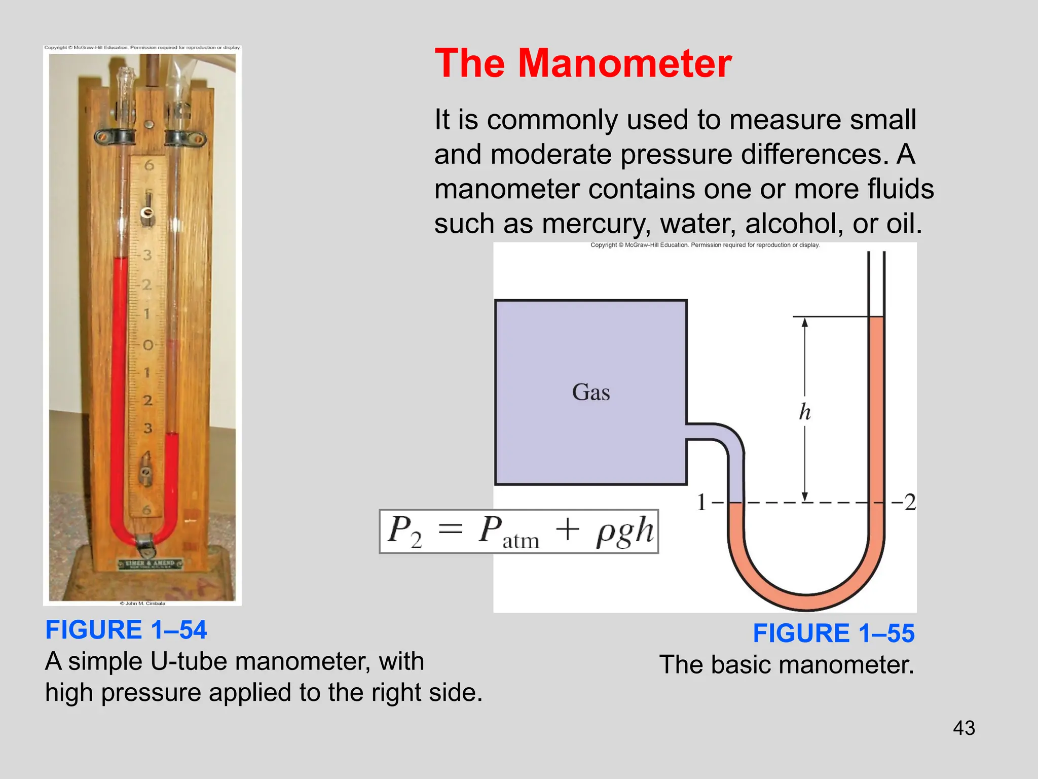
The Manometer
It is commonly used to measure small
and moderate pressure differences. A
manometer contains one or more fluids
such as mercury, water, alcohol, or oil.
FIGURE 1–55
The basic manometer.
FIGURE 1–54
A simple U-tube manometer, with
high pressure applied to the right side.

44. 44
FIGURE 1–57
In stacked-up fluid layers at rest, the
pressure change across each fluid
layer of density ρ and height h is ρgh.

45. 45
FIGURE 1–58
Measuring the pressure drop across
a flow section or a flow device by a
differential manometer.

46. 46
FIGURE 1–61
A deadweight tester can measure
extremely high pressures (up to 10,000
psi in some applications).

47. 47
PROBLEM-SOLVING TECHNIQUE
Step 1: Problem Statement
Step 2: Schematic
Step 3: Assumptions and Approximations
Step 4: Physical Laws
Step 5: Properties
Step 6: Calculations
Step 7: Reasoning, Verification, and Discussion

48. 48
FIGURE 1–63
The assumptions made while solving an
engineering problem must be
reasonable and justifiable.
FIGURE 1–62
A step-by-step approach can greatly
simplify problem solving.

49. 49
FIGURE 1–64
The results obtained from an
engineering analysis must be checked
for reasonableness.
FIGURE 1–65
Neatness and organization are highly
valued by employers.

50. 50
Engineering Software Packages
All the computing power and the
engineering software packages
available today are just tools,
and tools have meaning only in
the hands of masters.
Hand calculators did not
eliminate the need to teach our
children how to add or subtract,
and sophisticated medical
software packages did not take
the place of medical school
training.
Neither will engineering software
packages replace the traditional
engineering education. They will
simply cause a shift in emphasis
in the courses from mathematics
to physics.
FIGURE 1–66
An excellent word-processing
program does not make a person
a good writer; it simply makes a
good writer a more efficient writer.

51. 51
Despite its simplicity, Excel is commonly used in solving systems
of equations in engineering as well as finance. It enables the user
to conduct parametric studies, plot the results, and ask “what if ”
questions. It can also solve simultaneous equations if properly set
up.
Engineering Equation Solver (EES) is a program that solves
systems of linear or nonlinear algebraic or differential equations
numerically.
It has a large library of built-in thermodynamic property functions
as well as mathematical functions.
Unlike some software packages, equation solvers do not solve
engineering problems; they only solve the equations supplied by
the user.
Therefore, the user must understand the problem and formulate it
by applying any relevant physical laws and relations.
Equation Solvers

52. 52
A Remark on Significant Digits
In engineering calculations,
the information given is not
known to more than a certain
number of significant digits,
usually three digits.
Consequently, the results
obtained cannot possibly be
accurate to more significant
digits.
Reporting results in more
significant digits implies
greater accuracy than exists,
and it should be avoided. FIGURE 1–69
A result with more significant digits
than that of given data falsely implies
more precision.

53. 53
Summary
• Thermodynamics and energy
• Importance of dimensions and units
• Systems and control volumes
• Properties of a system
• Density and specific gravity
• State and equilibrium
• Processes and cycles
• Temperature and the zeroth law of thermodynamics
• Pressure
• The manometer
• The barometer and atmospheric pressure
• Problem solving technique