ผศ.ดร.ธีทัต ตรีศิริโชติ Page5
สำหรับเทคนิคที่ใช้ในกำรวิจัยเมื่อพิจำรณำจำกผลงำนที่ตีพิมพ์ในวำรสำรที่มี
ชื่อเสียง (Management Information Systems Quarterly [MISQ), Information Systems
Research [ISR], Journal of Management Information Systems [JMIS], and Journal of
the Association for Information Systems JAIS) ในช่วงปี ค.ศ. 2000-2008 พบว่ำส่วน
ใหญ่ ให้ควำมสำคัญในกำรใช้เทคนิคกำรวิเครำะห์ ยุคที่สอง (Gerow, Grover, Roberts,
& Thatcher, 2010) หลังจำกนั้นแล้วตั้งแต่ปี ค.ศ. 2005 เป็นต้นมำเริ่มมีกำรนำ PLS-SEM
มำใช้อย่ำงจริงจังเพรำะตัวโปรแกรมใช้ง่ำย ข้อมูลมีข้อจำกัดน้อย และให้ผลกำรวิเครำะห์
ในระดับที่ยอมรับได้ทำให้นักวิจัยได้ใช้ PLS-SEM มำกขึ้นอย่ำงเห็นได้ชัด (Ringle,
Sarstedt, & Straub, 2012)
ผศ.ดร.ธีทัต ตรีศิริโชติ Page14
Henseler, J., Ringle, C. M., & Sarstedt, M. (2012). Using Partial Least Squares Path Modeling in International Advertising Research:
Basic Concepts and Recent Issues. In S. Okazaki (Ed.), Handbook of Research in International Advertising (pp. 252–276). Cheltenham:
Edward Elgar Publishing.
15.
ผศ.ดร.ธีทัต ตรีศิริโชติ Page15
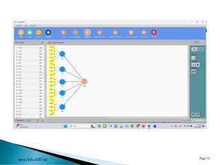
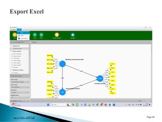
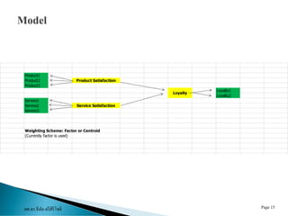
Product1
Product2
Product3
Loyalty1
Loyalty2
Service1
Service2
Service3
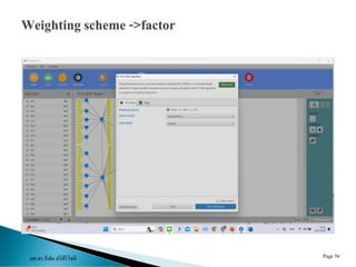
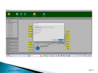
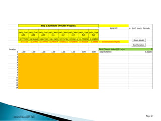
Weighting Scheme: Factor or Centroid
(Currently factor is used)
Product Satisfaction
Service Satisfaction
Loyalty
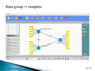
ผศ.ดร.ธีทัต ตรีศิริโชติ Page23
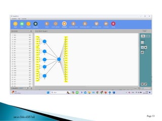
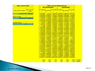
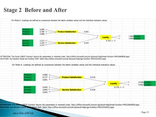
For Mode A: Loadings are defined as covariances between the latent variables values and the individual indicators values
Product1 0.880
Product2 0.798 0.502
Product3 0.888
1.808 Loyalty1
1.808 Loyalty2
Service1 2.213 0.754 <- r²
Service2 2.293 0.429
Service3 2.147
ATTENTION: The Excel-LINEST function returns the parameters in reversed order. http://office.microsoft.com/en-gb/excel-help/linest-function-HP010069838.aspx
ACHTUNG: Auf deutsch heisst die Funktion RGP. Siehe http://office.microsoft.com/de-de/excel-help/rgp-funktion-HP010342653.aspx
Product Satisfaction
Loyalty
Service Satisfaction
For Mode A: Loadings are defined as covariances between the latent variables values and the individual indicators values
Product1 0.896
Product2 0.777 0.510
Product3 0.891
0.938 Loyalty1
0.962 Loyalty2
Service1 0.843 0.776 <- r²
Service2 0.893 0.434
Service3 0.842
ATTENTION: The Excel-LINEST function returns the parameters in reversed order. http://office.microsoft.com/en-gb/excel-help/linest-function-HP010069838.aspx
ACHTUNG: Auf deutsch heisst die Funktion RGP. Siehe http://office.microsoft.com/de-de/excel-help/rgp-funktion-HP010342653.aspx
Product Satisfaction
Loyalty
Service Satisfaction
24.
ผศ.ดร.ธีทัต ตรีศิริโชติ Page24
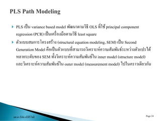
PLS เป็น variance based model พัฒนำตำมวิธี OLS ที่ใช้principal component
regression (PCR) เป็นเครื่องมือตำมวิธี least square
ตัวแบบสมกำรโครงสร้ำง (structural equation modeling, SEM) เป็น Second
Generation Model คือเป็นตัวแบบที่สำมำรถวิเครำะห์ควำมสัมพันธ์ระหว่ำงตัวแปรได้
หลำยระดับของ SEM ทั้งวิเครำะห์ควำมสัมพันธ์ใน inner model (structure model)
และวิเครำะห์ควำมสัมพันธ์ใน outer model (measurement model) ไปในครำวเดียวกัน
ผศ.ดร.ธีทัต ตรีศิริโชติ Page26
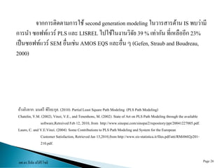
จำกกำรติดตำมกำรใช้ second generation modeling ในวำรสำรด้ำน IS พบว่ำมี
กำรนำ ซอฟท์แวร์ PLS และ LISREL ไปใช้ในงำนวิจัย 39 % เท่ำกัน ที่เหลืออีก 23%
เป็นซอฟท์แวร์ SEM อื่นเช่น AMOS EQS และอื่น ๆ (Gefen, Straub and Boudreau,
2000)
อ้ำงอิงจำก: มนตรี พิริยะกุล. (2010). PartialLeast Square Path Modeling (PLS Path Modeling)
Chatelin,Y.M. (2002), Vinzi, V.E., and Tenenhons, M. (2002). State of Art on PLS Path Modeling through the available
software,Retreived Feb 12, 2010, from http://www.sinopai.com/sinopai2/repository/ppt/20041227005.pdf.
Lauro, C. and V.E.Vinzi. (2004). Some Contributions to PLS Path Modeling and System for the European
Customer Satisfaction,RetrievedJan 13,2010,from http://www.sis-statistica.it/files.pdf/atti/RMi0602p201-
210.pdf.


![ผศ.ดร.ธีทัต ตรีศิริโชติ Page 4
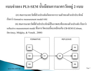
สถิติวิจัยยุคสอง แบ่งออกได้4 ประเภทคือ
(ก ) แบบจำลองสมกำรโครงสร้ำงฐำนควำมผันแปรร่วม (covariance base SEM
[CB-SEM) ใช้ได้ดีกับกำรพิสูจน์ สมมติฐำน/ทฤษฎี แต่ต้องมีจำนวนตัวอย่ำงที่มำกพอ
และข้อมูลต้องมีกำรกระจำยแบบปกติ (Wong, 2013)
(ข) แบบจำลองสมกำรโครงสร้ำงกำลังสองน้อยที่สุดเชิงส่วน ใช้เพื่อทดลองหำ
แบบจำลองที่เหมำะสม สำมำรถใช้กับตัวอย่ำงที่ไม่มำกนัก และ ข้อมูลไม่จำเป็นต้องมี
กำรกระจำยแบบปกติ (สุชำติ ประสิทธิ์รัฐสินธ์, 2557)
(ค) กำรวิเครำะห์องค์ประกอบ โครงสร้ำงทั่วไป (generalized structure
component analysis [GSCA]) ใช้เป็นตัวเลือกเมื่อ CB-SEM ไม่สำมำรถใช้ได้(Henseler,
2012) และ
(ง) แบบจำลองโครงสร้ำงสำกล (universal structured modeling [USM]) ใช้
วิเครำะห์ควำมสัมพันธ์ของตัวแปรที่เป็นเชิงเส้นและควำมสัมพันธ์ไม่เชิงเส้นได้
(Buckler, & Hennig-Thurau, 2008)](https://image.slidesharecdn.com/partialleastsquarepathmodelingwithsmartpls-240120093547-3939db6f/85/Partial-Least-Square-Path-Modeling-with-SmartPLS-4-320.jpg)
![ผศ.ดร.ธีทัต ตรีศิริโชติ Page 5
สำหรับเทคนิคที่ใช้ในกำรวิจัยเมื่อพิจำรณำจำกผลงำนที่ตีพิมพ์ในวำรสำรที่มี
ชื่อเสียง (Management Information Systems Quarterly [MISQ), Information Systems
Research [ISR], Journal of Management Information Systems [JMIS], and Journal of
the Association for Information Systems JAIS) ในช่วงปี ค.ศ. 2000-2008 พบว่ำส่วน
ใหญ่ ให้ควำมสำคัญในกำรใช้เทคนิคกำรวิเครำะห์ ยุคที่สอง (Gerow, Grover, Roberts,
& Thatcher, 2010) หลังจำกนั้นแล้วตั้งแต่ปี ค.ศ. 2005 เป็นต้นมำเริ่มมีกำรนำ PLS-SEM
มำใช้อย่ำงจริงจังเพรำะตัวโปรแกรมใช้ง่ำย ข้อมูลมีข้อจำกัดน้อย และให้ผลกำรวิเครำะห์
ในระดับที่ยอมรับได้ทำให้นักวิจัยได้ใช้ PLS-SEM มำกขึ้นอย่ำงเห็นได้ชัด (Ringle,
Sarstedt, & Straub, 2012)](https://image.slidesharecdn.com/partialleastsquarepathmodelingwithsmartpls-240120093547-3939db6f/85/Partial-Least-Square-Path-Modeling-with-SmartPLS-5-320.jpg)


![ผศ.ดร.ธีทัต ตรีศิริโชติ Page 33
สำหรับแบบจำลองที่ดีของ PLS-SEM แตกต่ำงจำก CB-SEM เพรำะแบบจำลอง
CB-SEM สร้ำงขึ้นจำกควำมพยำยำมทำให้ค่ำตำรำงควำมผันแปรร่วมของตัวแปร
ประจักษ์(manifest) ทั้งหมดที่ได้จำกข้อมูล และค่ำที่ได้จำกทฤษฎีมีค่ำเท่ำกัน ถือว่ำเป็น
ควำมเหมำะสมอย่ำงสมบูรณ์ของแบบจำลอง (perfect model fit)
ขณะที่แบบจำลอง PLS-SEM มำจำกควำมพยำยำมทำให้ค่ำกำรผันแปรของตัว
แปรแฝงแต่ละตัวที่หำได้จำกข้อมูล (แบบจำลองภำยนอก [outer model]) และจำกค่ำ
ทำนำย (แบบจำลองภำยใน [inner model]) มีค่ำเท่ำกัน (ทำให้บำงครั้งเรียก PLS-SEM ว่ำ
SEM ฐำนผันแปร(variance base) ด้วย
เหตุนี้กำรตรวจสอบควำมเหมำะสมของแบบจำลอง (model fit) ของ PLS-SEM
จึงเป็นกำรตรวจสอบแยกส่วนโดยตรวจสอบควำมเหมำะสมของแบบจำลองภำยนอก
และตรวจสอบควำมเหมำะสมของแบบจำลองภำยใน (Henseler, & Sarstedt, 2013) ไม่มี
กำรตรวจสอบควำมเหมำะสมของแบบจำลองในภำพรวม (global model fit) แต่ก็มี
นักวิจัยหลำยคนพัฒนำตัวชี้วัดในภำพรวมขึ้นมำเพื่อทำให้มองเห็นกำรเข้ำกับข้อมูลของ
แบบจำลองได้ดีขึ้น (Akter, D'Ambra.& Ray, 2011; Garson, 2016)](https://image.slidesharecdn.com/partialleastsquarepathmodelingwithsmartpls-240120093547-3939db6f/85/Partial-Least-Square-Path-Modeling-with-SmartPLS-33-320.jpg)