hjbjjjjjjjjjjjjjjjjjjjjjjjjjjjjjjjjjjjjjjj

1. See discussions, stats, and author profiles for this publication at: https://www.researchgate.net/publication/360076165
A Review of Sentiment Analysis of Tweets
Preprint · April 2022
DOI: 10.13140/RG.2.2.14283.67366/1
CITATIONS
0
READS
1,015
1 author:
Dhruvin Dankhara
University of Guelph
2 PUBLICATIONS 1 CITATION
SEE PROFILE
All content following this page was uploaded by Dhruvin Dankhara on 21 May 2022.
The user has requested enhancement of the downloaded file.

2. A Review of Sentiment Analysis of Tweets
Dhruvin Dankhara
(MEng): School of Engineering
University of Guelph
Guelph, Canada
(ddankhar@uoguelph.ca)
Abstract—Millions of people express their opinions and
thoughts about events, products or companies on online
platforms such as social networking sites, blogs, and forums.
The overall view of people’s sentiment can be useful to make
better decisions, measure effect of certain decisions or to
moderate content that may be harmful for the public. However,
the challenge is that the sentiment and views expressed by
people are in Natural Language, which is not understood by
computers. Also, the quantum of information is so large that the
task cannot be done manually. This paper shows how Natural
Language Processing (NLP), and Machine Learning (ML) can
be used to make accurate predictions of the underlying
sentiment of short texts such as a Tweet. We adopted two of the
main approaches used in text sentiment extraction – Lexicon
based approach and Text classification approach. However, we
observed the limitations of lexicon based approach for
classification of short texts such as Tweets as many of the Tweets
did not contain any lexicon from the dictionary. For the task of
text classification, we implemented K Nearest Neighbors,
Complement Naïve Bayes, Random Forests and Multi-Layer
Perceptron and Support Vector Machine algorithms on
processed tweets and achieved 76.7% accuracy with 80.7%
recall using support vector classifier. In this paper, we also
discuss the need of text preprocessing, tokenization and the
limitations of the methods used.
Keywords— Sentiment Analysis, Machine Learning, Natural
Language Processing, Social Media, Twitter Data, Vector
Representations, Sentiment Lexicons, Emotion Detection, Bag of
Words
I. INTRODUCTION
There has been a sharp increase in the reach of internet and
social media in recent past. Everyday millions of people post
on online platforms such as Twitter, Facebook, Reddit, Quora
and Instagram. The underlying information in the posts can be
useful to learn people’s opinion, feeling and perception
towards event, products, companies, and peoples. Previous
studied suggests that an opinion about any product, event or
service can essentially be reduced to a positive or a negative
sentiment associated with the text. [1] This knowledge can be
used to measure trust for a company or product [2] or build a
recommendation system [3] that recommends products or
services based on people’s current opinions and sentiments.
Sentiment analysis can be performed at many levels for the
text such as word level [4] [5], sentence level [6] [7],
document level [8] [9], and user level [10] [11]. Word level is
the lowest level of sentiment analysis that analyses word or
phrase to determine the overall sentiment of the text.
Similarly, sentence level analysis tries to associate single
sentiment to a sentence, document level sentiment analysis
looks at the overall sentiment of the whole document. User
level sentiment analysis is performed on users to find other
users holding similar sentiment.
However, sentiment analysis using computers poses
unique challenges as computers cannot understand text or
language. Careful preprocessing of data is needed to be able
to train machine learning algorithms on text derived from
social media as most of the data in social networks is
unstructured. [12] most tweets are written casually and
contains errors, spelling and grammatical mistakes, contextual
words, acronyms, special symbols, and URLs. Data cleaning
also serve as accuracy enhancement technique [13] and
feeding unnecessary data that does not contain any
information about sentiment of the tweet to machine learning
model will result in inaccurate predictions. However,
considering tweets are short text, excessive preprocessing can
remove almost all the text and we may be unable to derive any
meaningful conclusion from the remaining text. Hence, a
careful approach of removing unnecessary words and
formatting the important text is adopted in the preprocessing
phase.
Associating positive, neutral, or negative sentiment to a
text is called sentiment analysis. [14] There are three
approaches for text sentiment extraction – Lexicon-based
approach and machine learning based approach and linguistic
analysis. [15] Lexicon-based approach utilizes orientation
calculation for a text from semantics of the words in the text.
[16] The text classification approach uses labelled instances
of texts for building classifiers. [9] The linguistic method uses
the syntactic analysis of words and the text structure to
estimate sentiment of the text. [7]
Lexicon based approach uses sentiment lexicons which are
divided into two categories, corpus lexicon and dictionary
based lexicon. [17] Corpus lexicon are context oriented which
has two categories, semantic oriented and statistical oriented.
Dictionary based lexicon can be developed to contain words
that correlates to human emotions or words that are topic
oriented as described in [18]. For Jaccard similarity based
classifier used in this paper, we have adopted subjectivity
lexicon developed in [5] that contains words associated with
positive and negative sentiments.
Text classification approach employs supervised,
unsupervised, or semi-supervised machine learning methods
to classify texts based on underlying sentiments. Supervised
machine learning algorithms such as decision tree classifiers,
support vector machines (SVM), K nearest neighbor classifier
(KNN), neural network, Bayesian network and naïve bayes
uses labelled data to set mode parameters that defines decision
boundary separating classes and uses this model to make
accurate predictions for new data. Unsupervised machine
learning algorithms such as k-means uses unlabeled data to
cluster similar data into groups. This can be used to group
tweets with similar underlying sentiment. Another
classification of machine learning algorithm can be made as
linear classifier, probabilistic classifier and rule based
classifier depending on how the algorithm operates. Neural
network and support vector machine algorithms are linear as
boundary separating classes are defined by a linear
combination of features in data. Classifiers such as Naïve
Bayes and Bayesian distribution uses probability based

3. function to determine likelihood of data instance belonging to
certain class. Rule based classifier such as decision tree and k
nearest neighbor uses a rule based algorithm to accurately
identify similar instances.
II. METHODOLOGY
We have implemented two sperate approaches for tweet
classification. We have implemented sentiment lexicon based
approach using Jaccard similarity index and text classification
approach using CountVectorizer to capture the co-occurrence
of the words. The approaches are referred to as Sentiment
Lexicon-based classifier and Cooccurrence-based classifier
respectively in this report. Both approaches follow overall
similar methodology which can be summarized using flow
diagram shown in the figure 1. We have used Sentiment140
[19] dataset. We have not extracted new data from Twitter as
our main aim is to develop machine or identify machine
learning models that perform well for tweet sentiment
analysis. Sentiment140 dataset contains 6 columns with
sentiment label, tweet id, date and time, query, tweet author,
and tweet text. There are 1600,000 instances in the dataset.
However, we have used only 400,000 randomly selected
instances in this project. Data processing is very important
part of the whole process as the accuracy of the classifier is
highly dependent on the quality of the input data. We have
used SnowballStemmer and stopwords from Python library
nltk [20] for pre-processing of the tweets. Preprocessed tweets
are tokenized using keras [21] or nltk Tokenizer. Following
section provides detailed description of preprocessing. The
tokenized dataset is then sent to the algorithm for training and
prediction.
Fig. 1. Workflow of Sentiment Analysis
III. DATA PREPROCESSING & TOKENIZATION
Data pre-processing is the process of data cleaning and
preparation to make data suitable for classification. The tweets
usually contain a lot of noise and text that do not give any7
information about the sentiment of the tweet. Keeping such
text in the data not only increase the dimensionality of the
problem but also makes the decision making process more
difficult as the unnecessary data is also treated as one of the
features. Reducing noise in the data by pre-processing helps
increase the performance of the process and reduces the time
complexity of the algorithm. [22]
Preprocessing process involves following steps: Data
cleaning, white space removal, abbreviation expansion,
stemming, lamentation, stop words elimination, negation
handling and feature selection. The last step is referred to as
filtering while others are called transformations. Depending
upon the data and objective of the classification, some or all
the preprocessing steps may apply. Following are the
descriptions of the preprocessing techniques used in this
project.
1. Data Cleaning: Data cleaning part is mainly focused on
removing data that is not helpful in the decision making
and/or causes inaccuracies in the decision making process.
For the Twitter data this includes ‘@ mentions’, ‘# tags’,
hyperlinks, web addresses, special symbols, numbers and
emojis. Such data do not contain information regarding the
sentiment of the text and if they do, it is very difficult to
extract. Hence, such text is removed from the data. This
helps in decision making process as algorithm is not
affected by the noise.
2. White space removal: The data may also contain
whitespaces that can be considered as feature by the
algorithm if we are not careful. White spaces include
spaces, new lines, and tabs. All white space is replaced by
a single space that is not considered as feature in the
preprocessing part of the activity.
3. Stop Words Elimination: The articles, prepositions,
pronouns, conjunctions etc. are the features of language
that do not carry any meaning standalone and are used with
other words in the syntax. Few examples of such words are
‘the’, ‘a, ‘an’, ‘so’, ‘what’. Stop words do not carry any
information regarding the sentiment of the tweet and may
end up confusing the classifier if those are considered a
feature of the data. Also, the word that is accompanied by
the stop words usually contains the information of the text
sentiment. Hence, to reduce the data complexity and to
remove the noise in the data, stop words are removed from
the text. Figure 2 shows the tweet before and after applying
data cleaning, white space removal and stop words
elimination.
Fig. 2. Data after first phase of preprocessing
Data Collection
Data Pre-processing
Tokenization
Algorithm training
Prediction
Accuracy Calculation

4. 4. Tokenization: Tokenization is data transformation
method of breaking down text in to smaller unites called
tokens. There are three types of tokens, word, character
and subword tokens. For example, consider tokenization
of the text “Happiest memory”. Word tokenization of this
text will separate the text using space as delimiter and give
us ‘Happiest and ‘memory’. Character tokenization is done
at lower level which tokenizes the characters in a word.
This method tokenizes the word ‘Happiest: as h-a-p-p-i-e-
s-t. Lastly, subword tokenization attempts to split the word
into two tokens. For example, subword tokenization of
‘Happiest’ will give ‘Happy’ and ‘est’. Words are the
building blocks of the natural language and tokens are a
way of representing the words that can be used by
software. Often the tokens are represented by a unique
number instead of the text. This approach is helpful as
computers can handle numbers better than text and speed
of the program can be increased dramatically. In this
approach the whole text is converted into a word vector. It
may be helpful to limit the number of tokens by
considering only the most frequently repeated words to
reduce the dimensionality of the problem. Figure 3 shows
some of the tweets before and after tokenization.
Fig. 3. Tweets before and after tokenization
5. Bag of words Representation [23]: Bag of words
representation, as the name suggest is a method of writing
text as a bag of words that are present in it. This is useful
to identify which words usually occur together in a tweet
and represent the occurrence in a form that can be used by
machine learning model. This method creates a sparse
matrix that has all words in the dataset as column and all
instances in the dataset as row. If the word is present in the
instance, entry is written as 1, otherwise it is null. Hence,
using this method, text dataset can be converted into
feature dataset with words as feature. However, this
method does not consider grammar and word order of the
text. For instance, consider following set of text
Text = [‘hello my name is dhruvin’, ‘my research is on
tweet classification’]
This text contains two instances with five and six words
respectively. Table 1 shows the word count representation
of the given text and Table 2 shows index assignment to
words in dataset. It can be observed in table 1 for instance
2 that the order of words in the sentence is not preserved
but only the occurrence or the count of the word is
preserved.
Table 1: Word count representation of text data
Table 2: Token assignment to the words in text
Word Token
hello 1
my 2
name 3
is 4
dhruvin 5
research 6
on 7
tweet 8
classification 9
IV. SENTIMENT LEXICON-BASED CLASSIFIER
In lexicon-based classification, the text is assigned label
based on the count of words from the lexicons associated with
each label. If for the task of binary classification, we have
labels Y ∈ {0,1} we have lexicons W0 and W1. Then for the
instance with a vector of word counts x, the lexicon based
decision rule is given by the following equation. [24]
∑ 𝑥𝑖
𝑛
𝑖 ∈ 𝑊0
≷ ∑ 𝑥𝑗
𝑛
𝑗 ∈ 𝑊0
In this paper we use Jaccard similarity index to quantify
the similarity between the tweet and the lexicon corresponding
to positive or negative sentiment. Jaccard similarity index is a
measure of similarity between two sets of data. It is defined as
the ratio of the size of intersection and the size of the union of
two data sets as shown in the equation below. [25] [26]
𝐽(𝐴, 𝐵) =
|𝐴 ∩ 𝐵|
|𝐴 ∪ 𝐵|
In this classifier we have imported subjectivity lexicon
used by Theresa Wilson, Janyce Wiebe and Paul Hoffmann
[5] to build dictionary of positive keywords and negative
keywords. Figure 4 and figure 5 shows few entries of positive
sentiment lexicon and negative sentiment lexicon
respectively.
Token
Instance 1 2 3 4 5 6 7 8 9
0 1 1 1 1 1 0 0 0 0
1 1 0 0 1 0 1 1 1 1

5. Fig. 4. Positive Sentiment Lexicon
Fig. 5. Negative Sentiment Lexicon
This dictionary is also tokenized in similar manner to the
tweets. The algorithm calculates Jaccard similarity index
between tweet and the positive and negative dictionary. The
Jaccard index calculated are called positive scores and
negative scores respectively. Based on the sentiment scores of
the tweet, decision can be made that the tweet has positive
sentiment if positive score is higher, or the tweet has negative
sentiment if the negative score is higher. In the cases where
both scores are zero, a random class is assigned assuming that
not enough information available in the tweet to make
decision. Figure 6 shows the flow diagram for the algorithm.
Fig. 6. Flow chart of sentiment lexicon-based classifier
This simple classifier achieved 59.5% accuracy, which is
barely better than random guessing. One of the reasons the
classifier performed poorly is that almost 22.6% of the tweets
contained no keywords from the dictionary, hence algorithm
returned zero positive and negative scores. Refer figure 7 for
information of lexicon similarity scores for all tweets
Fig. 7. Lexicon similarity scores of tweets
Such instances are assigned random class, which affected
the performance of the algorithm significantly. Another more
fundamental drawback of the algorithm is that sentiment
analysis is a bit complicated than identifying keyword from
Tweet
Dataset
Preprocessing
Subjectivity Lexicon
Tokenized
Tweets
Positive
Dictionary
Negative
Dictionary
Jaccard
Function
Negative Score
Decision
Function
Preprocessing
Positive Score
Jaccard
Function
Output

6. the dictionary in the sentence. This classifier fails to
understand the semantics of the language. For example, “very
good” and “not good” are both the same thing for this
classifier as it only considers the keyword “good” and the
length of the sentence to calculate the Jaccard similarity index.
For this example, classifier will predict positive sentiment for
both the sentences, which is incorrect. Another major
drawback of this method is that it assigns equal weight to each
word in the text, but some words may be more important than
others. Supervised machine learning algorithms trained on
labeled data are likely to perform better than lexicon-based
classifiers due to their ability to identify complex relationships
between input features.
V. CO-OCCURRENCE BASED CLASSIFIER
Previous classifier performs poorly as it fails to account
for words in the tweet which are not present in the key-word
dictionary. Usually, meaning of the sentence depends largely
on the structure of the sentence rather than the key-words in
it. Another important point to note here is that similar texts
have similar words coexisting. As J. R. Firth said “You shall
know a word by the company it keeps” [27], we need a method
that can capture the co-occurrence of the words in tweets with
similar label. We can train a supervised machine learning
model that can learn the underlying relationship of co-
occurring words to make correct predictions about the
sentiment of the text.
One way to record co-occurrence is to convert the text to
a matrix of token counts. This method produces a sparse
matrix that counts the number of times a token is observed on
the text. We have used CountVectorizer from Scikit-learn [28]
to create such sparse matrix for our dataset which uses Scikit-
learn Tokenizer to convert text to tokens. The sparse matrix
can be viewed in a similar way to a regular machine learning
dataset where instances are tweets in the dataset and the
features are the tokenized words in the tweets. This similarity
makes it easy to train popular supervised machine learning
models. The dataset is split into training set and testing set
with the train to test ratio of 80% to 20%.
We have trained following five machine learning models
using training dataset.
(1) K Nearest Neighbors classifier [29]
(2) Complement Naïve Bayes Classifier [30]
(3) Random Forest Classifier [31]
(4) Multi-Layer Perceptron [32] and
(5) Support Vector Classifier [33]
Testing data is used to evaluate the accuracy of the model.
Random forest classifier achieves the maximum training
accuracy of 98.8% and support vector classifier achieves the
maximum testing accuracy of 75.52% among all classifiers
tested. Refer Figure 6 for the flow diagram of the process.
Although this method gives reasonable performance, it
still fails to understand the semantics of the language. Which
means it will give false prediction when presented with
ambiguous or sarcastic text.
Fig. 8. Flow chart of Co-occurrence-Based Classifier
VI. RESULTS AND DISCUSSIONS
Measures of Performance
The basic concept in evaluation of machine learning model
is the error. If the class predicted by the classifier is different
from the actual class, then it is defined as an error in
classification. The ratio of correctly classified instances to
total number of test cases is called accuracy. Accuracy can be
used to measure the performance of the classifier in case when
any mistake is equally important.
𝐴𝑐𝑐𝑢𝑟𝑎𝑐𝑦 =
Number of correct classifications
Total number of test cases
The primary disadvantages of accuracy are that it does not
make any distinction between the types of error, and it is
highly dependent on the class distribution in the dataset. For
example, in the binary classification case with 90% negative
instances and 10% positive instances, random guessing will
also result in accuracy score of 90%, which is not useful.
However, in our case the class distribution is around 50% and
any error is equally important, accuracy can be used as a useful
metric for evaluation.
For classification task, accuracy portrays incomplete
picture of the performance of the model. Accuracy of
classifier do not give any information regarding the mistakes
done by the classifier. Precision and recall are used to describe
the performance of the classifier in mode depth. Consider
typical confusion matrix for binary classification problem in
Table 3. Classification by the model falls into four categories,
True Positive (TP), True Negative (TN), False Positive (FP)
and False Negative (FN) where positive and negative refers to
Prediction
Tweet Dataset
Preprocessing
Tokenized Tweets
Count Vectorizer
Sparse Matrix of
Word count
Machine Learning
Model
Training Data
Testing
Data

7. class of the instance and true and false refers to correctness of
the model’s prediction. This information is used to calculate
precision, recall and F1 score for the classifier.
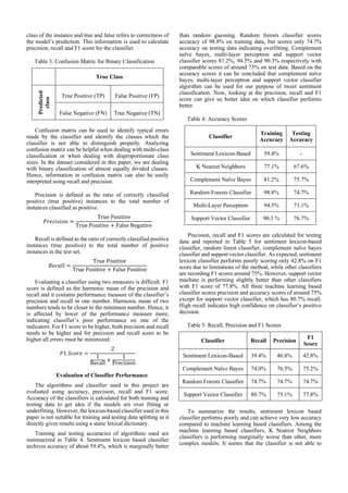
Table 3: Confusion Matric for Binary Classification
True Class
Predicted
class
True Positive (TP) False Positive (FP)
False Negative (FN) True Negative (TN)
Confusion matrix can be used to identify typical errors
made by the classifier and identify the classes which the
classifier is not able to distinguish properly. Analyzing
confusion matrix can be helpful when dealing with multi-class
classification or when dealing with disproportionate class
sizes. In the dataset considered in this paper, we are dealing
with binary classification of almost equally divided classes.
Hence, information in confusion matrix can also be easily
interpreted using recall and precision.
Precision is defined as the ratio of correctly classified
positive (true positive) instances to the total number of
instances classified as positive.
𝑃𝑟𝑒𝑐𝑖𝑠𝑖𝑜𝑛 =
True Positive
True Positive + False Negative
Recall is defined as the ratio of correctly classified positive
instances (true positive) to the total number of positive
instances in the test set.
𝑅𝑒𝑐𝑎𝑙𝑙 =
True Positive
True Positive + False Positive
Evaluating a classifier using two measures is difficult. F1
score is defined as the harmonic mean of the precision and
recall and it contains performance measure of the classifier’s
precision and recall in one number. Harmonic mean of two
numbers tends to be closer to the minimum number. Hence, it
is affected by lower of the performance measure more,
indicating classifier’s poor performance on one of the
indicators. For F1 score to be higher, both precision and recall
needs to be higher and for precision and recall score to be
higher all errors must be minimized.
𝐹1 𝑆𝑐𝑜𝑟𝑒 =
2
1
Recall
+
1
Precision
Evaluation of Classifier Performance
The algorithms and classifier used in this project are
evaluated using accuracy, precision, recall and F1 score.
Accuracy of the classifiers is calculated for both training and
testing data to get idea if the models are over fitting or
underfitting. However, the lexicon-based classifier used in this
paper is not suitable for training and testing data splitting as it
directly gives results using a static lexical dictionary.
Training and testing accuracies of algorithms used are
summarized in Table 4. Sentiment lexicon based classifier
archives accuracy of about 59.4%, which is marginally better
than random guessing. Random forests classifier scores
accuracy of 98.8% on training data, but scores only 74.7%
accuracy on testing data indicating overfitting. Complement
naïve bayes, multi-layer perceptron and support vector
classifier scores 81.2%, 94.5% and 90.3% respectively with
comparable scores of around 75% on test data. Based on the
accuracy scores it can be concluded that complement naïve
bayes, multi-layer perceptron and support vector classifier
algorithm can be used for our purpose of tweet sentiment
classification. Now, looking at the precision, recall and F1
score can give us better idea on which classifier performs
better.
Table 4: Accuracy Scores
Classifier
Training
Accuracy
Testing
Accuracy
Sentiment Lexicon-Based 59.4% -
K Nearest Neighbors 77.1% 67.6%
Complement Naïve Bayes 81.2% 75.7%
Random Forests Classifier 98.8% 74.7%
Multi-Layer Perceptron 94.5% 73.1%
Support Vector Classifier 90.3 % 76.7%
Precision, recall and F1 scores are calculated for testing
data and reported in Table 5 for sentiment lexicon-based
classifier, random forest classifier, complement naïve bayes
classifier and support vector classifier. As expected, sentiment
lexicon classifier performs poorly scoring only 42.8% on F1
score due to limitations of the method, while other classifiers
are recording F1 scores around 75%. However, support vector
machine is performing slightly better than other classifiers
with F1 score of 77.8%. All three machine learning based
classifier scores precision and accuracy scores of around 75%
except for support vector classifier, which has 80.7% recall.
High recall indicates high confidence on classifier’s positive
decision.
Table 5: Recall, Precision and F1 Scores
Classifier Recall Precision
F1
Score
Sentiment Lexicon-Based 39.4% 46.8% 42.8%
Complement Naïve Bayes 74.0% 76.5% 75.2%
Random Forests Classifier 74.7% 74.7% 74.7%
Support Vector Classifier 80.7% 75.1% 77.8%
To summarize the results, sentiment lexicon based
classifier performs poorly and can achieve very low accuracy
compared to machine learning based classifiers. Among the
machine learning based classifiers, K Nearest Neighbors
classifiers is performing marginally worse than other, more
complex models. It seems that the classifier is not able to

8. identify the similarity between tweets as tweets are very short
set of words and there are relatively huge number of words in
the dataset, making finding similar neighbor difficult. Other
machine learning classifiers can identify underlying
relationship between tweets of similar sentiment and are able
to distinguish them using complex decision boundary.
VII. CONCLUSION
We observed that to be able to make accurate prediction
for text data, it is not enough to look at the words in the text in
isolation. Classifier which focuses on only finding key-words
to make prediction about text often fails as either it is not able
to find any keyword, or the meaning of the text is different due
to semantics, despite presence of the key-words in the text.
Another type of classifiers is based on machine learning
methods, which can build relationships between text and class
based on the co-occurrences of certain words in the text. This
classifier performed significantly better in our task of binary
classifier and can be used in many practical applications,
keeping the limitation of the classifier in mind. Even though
this classifier performs reasonably well, it cannot understand
the semantics of the language. Predictions by this classifier are
based on building statistical relationship using machine
learning model. The performance of both kinds of classifiers
is highly affected by the input data and hence on the pre-
processing of the data. Careful preprocessing shall ensure
complete elimination of noise without removing any
important features. Performance sentiment lexicon-based
classifier is dependent on the lexicon dictionaries and
optimization of the dictionary can increase the performance of
such classifier. Lexicon dictionary generated using the dataset
can be implemented to reduce the chances cases with zero
Jaccard similarity index, increasing the performance of the
sentiment lexicon-based classifier. There are advanced
transformers based language models such as BERT (Bi-
directional Encoder Representation from Transformers)
which can understand syntax and semantics of the language
and are likely to perform better at sentiment classification
task.
REFERENCES
[1] B. Liu, "Web Data Mining: Exploring Hyperlinks,
Contents, and Usage Data," Springer, 2006.
[2] S. Yosaphine, A. Livingstone, B. Chin Ng and E.
Cambria, "The Hourglass Model Revisited," IEEE
Intelligent Systems, vol. 35, no. 5, pp. 96-102, 2020.
[3] D. Yang, D. Zhang, Z. Yu and Z. Wang, "A
sentiment-enhanced personalized location
recommendation system," in Proceedings of the 24th
ACM Conference on Hypertext and Social Media,
2013.
[4] P. Tetlock, M. Saar-Tsechnasky and S. Macskassy,
"More than words: Quantifying language to measure
firms' fundamentals," The Journal of Finance, vol.
63, no. 3, pp. 1437-1467, 2008.
[5] W. Theresa, W. Janyce and H. Paul, "Recognizing
contextual polarity in phrase-level sentiment
analysis," in HLT-EMNLP, 2005.
[6] H. Yu and V. Hatzivassiloglou, "Towards answering
opinion questions: separating facts from opinions and
identifying the polarity of opinion sentences," in
Empirical methods in natural language processing,
2003.
[7] L. Tan, J. Na, Y. Theng and K. Chang, "Sentence-
level sentiment polarity classification using a
linguistic approach, Digital Libraries," Cultural
Heritage, Knowledge Dissemination, and Future
Creation, pp. 77-87, 2011.
[8] S. R. Das, "News Analytics: Framework, Techniques
and Metrics," in the Handbook of News Analytics in
Finance, Wiley Finance, 2010.
[9] B. Pang, L. Lee and S. Vaithyanathan, "Thumbs up?
Sentiment Classification using Machine Learning
Techniques," Proceedings of the 2002 Conference on
Empirical Methods in Natural Language Processing
(EMNLP 2002), pp. 79-86, 2002.
[10] P. Melville, W. Gryc and R. Lawrence, "Sentiment
analysis of blogs by combining lexical knowledge
with text classification," in ACM SIGKDD
international conference on Knowledge discovery and
data mining, 2009.
[11] C. Tan, L. Lee, J. Tang, L. Laing, M. Zhou and P. Li ,
"User-level sentiment analysis incorporating social
networks," Arxiv preprint.
[12] Y. Ko and J. Seo, "Automatic Text Categorization by
Unsupervised Learning," Association for
Computational Linguistics, no. 18, pp. 453-459,
2000.
[13] A. K. Uysal and S. Gunal, "The impact of
preprocessing on text classification," Information
Processing & Management, vol. 50, no. 1, pp. 104-
112, 2014.
[14] W. Medhat, A. Hassan and H. Korashy, "Sentiment
analysis algorithms and applications: A survey," Ain
Shams Engineering Journal, vol. 5, no. 4, pp. 1093-
1113, 2014.
[15] M. Thelwall, K. Buckley and G. Paltoglou,
"Sentiment in twitter events," American Society for
Information Science and Technology, vol. 62, no. 2,
pp. 406-418, 2011.
[16] P. D. Turney, "Thumbs Up or Thumbs Down?
Semantic Orientation Applied to Unsupervised
Classification of Reviews," in Association for
Computational Linguistics (ACL), Philadelphia, 2002.
[17] N. El-Fishawy, A. Hamouda, G. M. Attiya and M.
Atef, "Arabic summarization in Twitter social
network," Ain Shams Engineering Journal, vol. 5, no.
2, pp. 411-420, 2014.
[18] M. Taboada, J. Brooke, M. Tofiloski, K. Voll and M.
Stede, "Lexicon-Based Methods for Sentiment
Analysis," Computational Linguistics, vol. 37, no. 2,
pp. 267-307, 2011.
[19] "Sentiment140," [Online]. Available:
http://help.sentiment140.com/for-students.
[20] S. Bird, E. Klein and E. Loper, Natural language
processing with Python: analyzing text with the
natural language toolkit, Reilly Media, Inc., 2009.

9. [21] F. Chollet, "Keras," 2015. [Online]. Available:
https://keras.io.
[22] E. Haddi, L. Xiaohui and S. Yong, "The Role of Text
Pre-processing in Sentiment Analysis," Information
Technology and Quantitative Management
(ITQM2013), vol. 17, pp. 26-32, 2013.
[23] Z. S. Harris, "Distributional Structure," Word, vol. 10,
no. 2-3, pp. 146-162, 1954.
[24] J. Enisenstein, "Unsupervised Learning for Lexicon-
Based Classification," in Proceedings of the Thirty-
First AAAI Conference on Artificial Intelligence.
[25] P. Jaccard, "The distribution of the floura in the
alpine zone," New Phytologist Foundation, vol. 11,
no. 2, pp. 27-50, 1912.
[26] TT, Tanimoto, "An elementary mathematical theory
of classification and prediction," Internal IBM
Technical Report, 1958.
[27] J. R. Firth, "Applications of General Linguistics," in
Transactions of the Philological Society, 1957.
[28] Pedregosa et al., "Scikit-learn: Machine Learning in
Python," Journal of Machine Learning Research, no.
12, pp. 2825-2830, 2011.
[29] E. Fix, Hodges and L. Joseph, "Discriminatory
Analysis. Nonparametric Discrimination: Consistency
Properties," USAF School of Aviation Medicine,
Rnadoplh Field, Texas, 1951.
[30] A. McCakkum, "Graphical Models, Lecture2:
Bayesian Network Representation," 2019. [Online].
Available:
https://people.cs.umass.edu/~mccallum/courses/gm20
11/02-bn-rep.pdf.
[31] H. Tin Kam, "Random Decision Forests," in
International conference on DOcument Analysis and
Recognition , Montreal, QC, 1995.
[32] Hastie, T. Tibshirani and J. Friedman, "The elements
of Statistical Learning: Data Mining, Inference and
Prediction," Springer, 2009.
[33] C. Cortes and V. Vladimir, "Support-vector
networks," Machine Learning, vol. 20, pp. 273-297,
1995.
[34] R. Socher, F. Chaubard and R. Mundra, "CS 224D:
Deep Learning for NLP," 2016. [Online]. Available:
https://cs224d.stanford.edu/lecture_notes/notes1.pdf.
View publication stats