Download as PDF, PPTX

![/ xx
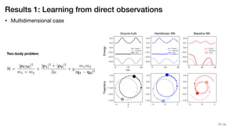
Results 1: Learning from direct observations
Ideal Harmonic Oscillator
Ideal Pendulum
Real Pendulum
Schmidt & Lipson [35]
Learned Hamiltonian
Ground Truth Hamiltonian
!9](https://image.slidesharecdn.com/hamiltoniannn-200131102421/85/Paper-reading-Hamiltonian-Neural-Networks-9-320.jpg)
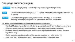

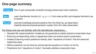
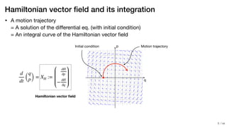
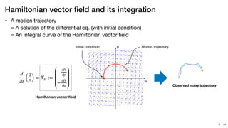
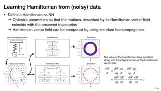
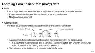
- Standard machine learning models do not guarantee satisfying physical conservation laws for motion prediction. - The paper proposes learning the "equations of motion" in the form of a Hamiltonian function using neural networks to predict trajectories that obey conservation laws. - The learned Hamiltonian function is integrated on the fly to generate predictions, ensuring the predictions satisfy conservation of energy.


![MATEBELE A MOLETLANE (BA BINA TLOU)[1].pptx](https://cdn.slidesharecdn.com/ss_thumbnails/matebeleamoletlanebabinatlou1-251010112533-8ce8c638-thumbnail.jpg?width=640&height=640&fit=bounds)


![Polymer [ बहुलक ] Chemistry Notes PDF - Irfanullah Mehar - JJ Sir Chemistry.pdf](https://cdn.slidesharecdn.com/ss_thumbnails/polymerchemistrynotespdf-irfanullahmehar-jjsirchemistry-260210172118-3f9b37f7-thumbnail.jpg?width=640&height=640&fit=bounds)