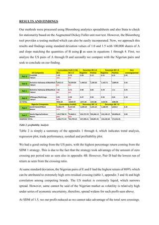
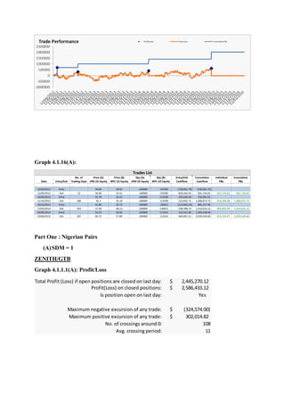
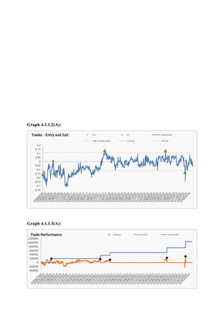
The document summarizes an investigation into pairs trading to profit from arbitrage opportunities. The author selects pairs of securities from the US and Nigerian markets, tests for cointegration using the Engle-Granger approach, and develops a pairs trading strategy based on the residual plot. Using standard deviation thresholds of 1.0 and 1.5, the strategy is applied to the selected pairs and performance is analyzed, finding profits from 109-809% for the Nigerian pairs and 45-106% for the US pairs. The author concludes pairs trading can be profitable in both advanced and developing markets but notes future research could incorporate transaction costs and more fully examine excursion effects.
Statistical Arbitrage
Pairs Trading, Long-Short Strategy
Cyrille BEN LEMRID

1 Pairs Trading Model 5
1.1 Generaldiscussion ................................ 5 1.2 Cointegration ................................... 6 1.3 Spreaddynamics ................................. 7
2 State of the art and model overview 9
2.1 StochasticDependenciesinFinancialTimeSeries . . . . . . . . . . . . . . . 9 2.2 Cointegration-basedtradingstrategies ..................... 10 2.3 FormulationasaStochasticControlProblem. . . . . . . . . . . . . . . . . . 13 2.4 Fundamentalanalysis............................... 16
3 Strategies Analysis 19
3.1 Roadmapforstrategydesign .......................... 19 3.2 Identificationofpotentialpairs ......................... 19 3.3 Testingcointegration ............................... 20 3.4 Riskcontrolandfeasibility............................ 20
4 Results
22
2
Contents

Introduction
This report presents my research work carried out at Credit Suisse from May to September 2012. This study has been pursued in collaboration with the Global Arbitrage Strategies team.
Quantitative analysis strategy developers use sophisticated statistical and optimization techniques to discover and construct new algorithms. These algorithms take advantage of the short term deviation from the ”fair” securities’ prices. Pairs trading is one such quantitative strategy - it is a process of identifying securities that generally move together but are currently ”drifting away”.
Pairs trading is a common strategy among many hedge funds and banks. However, there is not a significant amount of academic literature devoted to it due to its proprietary nature. For a review of some of the existing academic models, see [6], [8], [11] .
Our focus for this analysis is the study of two quantitative approaches to the problem of pairs trading, the first one uses the properties of co-integrated financial time series as a basis for trading strategy, in the second one we model the log-relationship between a pair of stock prices as an Ornstein-Uhlenbeck process and use this to formulate a portfolio optimization based stochastic control problem.
This study was performed to show that under certain assumptions the two approaches are equivalent.
Practitioners most often use a fundamentally driven approach, analyzing the performance of stocks around a market event and implement strategies using back-tested trading levels.
We also study an example of a fundamentally driven strategy, using market reaction to a stock being dropped or added to the MSCI World Standard, as a signal for a pair trading strategy on those stocks once their inclusion/exclusion has been made effective.
This report is organized as follows. Section 1 provides some background on pairs trading strategy. The theoretical results are described in Section 2. Section 3
Explicamos de una manera muy muy sencilla lo que es el arbitraje estadistico y el pairs trading y como se puede operar manual y automaticamente con expert advisors.
This document provides an introduction to pair trading based on cointegration. It discusses that pair trading selects two highly correlated stocks and trades their price differences. Cointegration refers to the long-term co-movement of stock prices, which pair trading exploits. The document outlines the basic idea of pair trading when stock prices diverge, and simulates pair trading using R language to estimate spreads, check for cointegration, generate signals, and backtest performance. In summary, pair trading is a quantitative strategy that aims to profit from mean reversion of cointegrated stock price spreads.
The document describes a pairs trading model and software implementation in three parts:
1. It outlines four mathematical methods - normalized differences, cointegration, stochastic spread, and time varying mean reversion - to analyze pair spreads and generate trading signals.
2. It discusses how the accompanying software add-in allows running the computationally intensive methods in EViews and producing summary outputs, charts, and test results.
3. It provides examples of the add-in interface and sample trading signal and statistical output to demonstrate the model's application and usefulness for financial decision making despite some limitations.
Join CMT Level 1, 2 & 3 Program Courses & become a professional Technical Analyst, CMT USA Best COACHING CLASSES. CMT Institute Live Classes by Expert Faculty. Exams are available in India. Best Career in Financial Market.
https://www.ptaindia.com/chartered-market-technician/
Forward contracts allow parties to lock in an exchange rate for buying or selling an asset at a future date. There are several types of forward contracts including currency forwards. Currency forwards are used by importers, exporters, investors and borrowers to hedge against currency risk. Forward rates are determined based on interest rate differentials between currencies under the principle of covered interest rate parity.
The document provides a history of the development of the Indian equity derivatives market from 2000 to 2007. It discusses key milestones such as the launch of index futures, index options, and stock futures/options on the National Stock Exchange and Bombay Stock Exchange. The document also outlines the main features of derivatives trading in India such as the exchanges involved, trading systems, margin requirements, and typical volumes. Examples of records achieved in futures and options segments are also presented.
Derivatives derive their value from underlying assets such as stocks, commodities, currencies, and bonds. The main types of derivatives are forwards, futures, and options. Forwards involve an obligation for both parties to fulfill the contract terms at a future date. Futures are standardized contracts traded on an exchange with high liquidity. Options confer the right but not obligation to buy or sell the underlying asset at a strike price by an expiry date. Key participants in derivatives markets include speculators, hedgers, and arbitrageurs. Common derivatives strategies involve futures arbitrage, hedging, and using options spreads. Greeks like delta and gamma help analyze how option prices change with movements in the underlying asset.
Este documento presenta una guía de análisis técnico que explica conceptos básicos como qué es el análisis técnico, los diferentes tipos de gráficos, y marcos temporales. También cubre patrones como tendencias, soportes, resistencias, correcciones, y figuras como triángulos, banderas y dobles suelos/techos. Finalmente, introduce conceptos de Fibonacci y ondas de Elliot para ayudar en el análisis técnico.
The Tokyo Stock Exchange (TSE) is the third largest stock exchange in the world. It was founded in 1878 and as of 2011 had a market capitalization of $3.3 trillion. In 2013, it merged with the Osaka Securities Exchange to form the Japan Exchange Group. The TSE has over 2,200 listings, including both domestic Japanese companies and some foreign companies. It is divided into first, second, and Mothers sections for large, mid-sized, and high-growth startup companies respectively. Major indices that track the TSE include the Nikkei 225 and TOPIX indexes. In addition to stocks, the TSE also offers trading in derivatives like futures, options, and ETFs.
The National Stock Exchange of India (NSE) is the largest stock exchange in India. It was established in 1992 as the first demutualized electronic exchange. [NSE provides a modern, automated, electronic trading system and was the first to offer online trading access nationwide.] It introduced transparency to market trading by separating exchange management from ownership. NSE facilitates trading in equities, derivatives, debt instruments, mutual funds and more. The Nifty 50 index tracks the top 50 Indian companies listed on NSE. Trading occurs on all days except weekends and holidays from 9:15 am to 3:30 pm.
Quant insti webinar on algorithmic trading for technocrats!QuantInsti
The webinar links the key concepts of Algorithmic Trading to Engineers and Technology Graduates. It is aimed at explaining Algo Trading Basics in way that is easily understandable and palatable.
This video is part of a webinar taken by Gaurav Raizada on 14th May, 2013 at QuantInsti, Mumbai. The webinar was about Algorithmic and High Frequency trading career for technocrats with detailed discussion about this domain and different skill sets required to excel in this industry.
The document summarizes key aspects of foreign exchange markets. It discusses that the forex market is a decentralized global market for trading currencies that operates 24 hours a day. The largest forex markets are located in London, New York, Tokyo, Zurich, and Frankfurt. It also notes that India's foreign exchange reserves reached $360 billion in March 2016. The reserves help with monetary policy, exchange rates, providing liquidity and buffer against external factors, and earning subsidiary revenue. The document outlines the different types of forex markets including merchant, inter-bank, and international markets and lists some common participants. It also describes exchange rate mechanisms and derivatives used to manage foreign exchange risk.
For full text article go to : https://www.educorporatebridge.com/forex/forex-trading/ Have you ever wondered about the, import-export happening in the countries? Are you new to the concept of Forex Trading? Here is an article on forex trading which will explain you about the Forex Market like why Foreign Exchange happens? , different ways to trade forex, and risks involved in forex trading.
The document provides an overview of technical analysis tools including moving averages, the Average Directional Index (ADX), and derivatives. It defines moving averages as indicators that smooth price data to identify trends, discussing simple and exponential moving averages. It explains how the ADX measures trend strength without direction, using the Plus Directional Indicator (+DI) and Minus Directional Indicator (-DI) to define direction. Finally, it introduces derivatives such as forwards, futures, and options contracts, defining basic terminology used in derivatives trading like strike price and intrinsic value.
An options contract gives the buyer the right, but not the obligation, to buy or sell an underlying asset at a specified strike price on or before the expiration date. There are call and put options. A call option allows buying the asset, while a put option allows selling the asset. The buyer pays a premium to the seller for this right. The profit/loss of the buyer and seller depends on whether the option expires in or out of the money. The buyer's potential profit is unlimited but their loss is limited to the premium paid, whereas for the seller the potential loss is unlimited but profit is limited to the premium received.
This document defines derivatives and describes their key features and types. It explains that a derivative is a financial instrument whose value is based on an underlying asset. The main types of derivatives discussed are forwards, futures, swaps, and options. It provides examples of each type and outlines their key characteristics. It also discusses derivative markets in Pakistan and how derivatives can help reduce risk but also enable speculation.
Floating exchange rate system in indiaHimani Gupta
The document discusses India's managed floating exchange rate system where the value of the rupee is determined by market forces in the foreign exchange market but the central bank intervenes during extreme fluctuations to minimize currency value changes. It provides a history of India's exchange rate regimes from 1947 to 1993 when it transitioned to a market-determined system. Tables show the annual average exchange rate of the rupee against the US dollar from 1993 to 2013, which generally depreciated over time except for some appreciation periods. The document also discusses the effects of rupee appreciation and depreciation on imports, exports, inflation and the balance of payments.
Day trading techniques include scalping, fading, daily pivots, and momentum trading. Scalping aims to take quick profits by entering and exiting positions as soon as they become profitable. Fading shorts a stock when it moves up quickly, expecting a sell-off. Daily pivots look to benefit from volatility by buying low and selling high, exiting on signs of reversal. Momentum trades ride trends fueled by news or volume until signs of reversal like decreasing volume or bearish candles. Day traders use candlestick charts, level 2 quotes, and newsfeeds to identify entry points supported by patterns, volume spikes, and order book depth.
The document discusses foreign exchange markets, including the types of transactions that occur, participants, and how exchange rates are determined. It covers the functions of foreign exchange markets in facilitating international trade and investments. Exchange rates can be fixed or floating. India moved to a dual exchange rate system in 1992 that allowed partial convertibility of the rupee, with some transactions occurring at the market rate and others at an official rate, in order to make foreign exchange available for essential imports. Full convertibility was later introduced.
This document provides an overview of hedging strategies using options. It discusses using protective puts when long on a stock to minimize downside risk. It also discusses covered calls, where an investor long on a stock can sell call options to generate income and reduce their cost basis if the stock remains flat. The document also introduces bull call spreads and bear put spreads as directional strategies to benefit from upside in a bullish view or downside in a bearish view, while limiting risk. Examples are provided to illustrate each strategy.
Technical and fundamental analysis on stock market Babasab Patil
The document discusses technical and fundamental analysis of securities. It provides an overview of technical analysis concepts like Dow theory, Elliot waves, and moving averages. It also discusses fundamental analysis, including economic, industry, and company analysis. Key company analysis factors mentioned include management, annual reports, ratios, and cash flow. The document outlines objectives to conduct technical and fundamental analysis of selected Indian stock market securities. It describes the research methodology as involving secondary data analysis and a sample size of 10 stocks for technical analysis and 4 for fundamental analysis.
The Dow Theory originated with Charles Dow and analyzes stock market movements on three levels - daily fluctuations, secondary trends lasting weeks to months, and primary trends spanning multiple years. These trends are compared to ripples, waves, and tides respectively. The theory holds that markets discount all information and move through bull and bear cycles shown by peaks and troughs in the primary trend. Support and resistance levels also factor in where demand or supply prevents further price changes. However, the Dow Theory is not infallible and is based on historical interpretation of data rather than a scientific theory.
Module - 1 :
The foreign exchange market, structure and organization- mechanics of currency trading
– types of transactions and settlement dates – exchange rate quotations and arbitrage – arbitrage with and without transaction costs – swaps and deposit markets – option forwards – forward swaps and swap positions – Interest rate parity theory.
The document discusses foreign exchange rates and international trade from a lecture on the topic. It defines exchange rates and how they allow prices in different currencies to be compared. It also discusses the foreign exchange market, how exchange rates are determined, and different types of exchange rate agreements like spot rates, forward rates, and currency swaps. Real exchange rates account for differences in purchasing power between countries. Equilibrium exchange rates occur when supply and demand for a foreign currency are equal.
instruments of Money market and capital marketVikash Gupta
This document provides an overview of various financial instruments traded in the money market and capital market in India. It defines key terms like money market, capital market, and describes common instruments like treasury bills, commercial paper, debentures and bonds. In the money market, short term instruments like treasury bills, certificates of deposit, and commercial bills are traded. The capital market deals in long term instruments like stocks, debentures and bonds. Preference shares and equity shares are also discussed and compared.
This document provides an overview of financial derivatives, including:
- A derivative is a financial instrument whose value is derived from an underlying asset. Common types of derivatives include forwards, futures, options, and swaps.
- Derivatives can be traded over-the-counter (OTC) between two parties or on an exchange.
- In Pakistan, derivatives on financial assets trade on the Pakistan Stock Exchange, while commodity derivatives trade on the Pakistan Mercantile Exchange.
This document summarizes a student paper on the low-volatility anomaly. The paper examines whether low-volatility stocks achieve higher risk-adjusted returns compared to predictions of CAPM and MPT. It reviews literature explaining the anomaly through various behavioral biases. The paper tests the anomaly using 30 S&P 500 stocks over 20 years. Regression analysis finds no significant relationship between past stock volatility and future returns, providing no support for either CAPM or the low-volatility anomaly based on the sample. Statistical tests confirm the results and inability to reject the null hypothesis of no relationship between risk and return.
This document discusses future contracts and the binomial tree model for pricing derivatives. It analyzes the stock prices of Apple and Facebook to compare theoretical forward prices to observed future prices. For Apple, the theoretical forward price is calculated and compared to the future price, finding small differences. For Facebook, future and spot prices are analyzed and seen to converge at maturity as expected. The second part uses the binomial tree model to calculate prices and delta values for European call and put options on the underlying asset. It finds that option prices increase with more periods to maturity but decrease as expiration approaches. The model is also used to price American put options and compare to European puts.
1. The document analyzes value and growth stocks between 1975-2004, comparing their returns and risks. It finds that value stocks generally outperformed growth stocks over this period.
2. A moving average analysis of the value-growth return spread shows it fluctuated between positive and negative returns with no clear pattern, contradicting the theory that value stocks always outperform. The spreads were also small relative to the portfolios' volatility.
3. Regression analyses found the CAPM model did not accurately predict returns. The growth portfolio underperformed predictions by -0.15% annually, while the value portfolio outperformed by 0.14%, contradicting CAPM. The spread portfolio had low correlation to the market, as
This document examines stock market volatility in the US and BRICS countries using GARCH models. Statistical analysis of daily stock returns from 2010-2015 finds the volatility varies among the six countries and is often asymmetric. The US stock market showed the most stability and highest average returns, while Russia and South Africa had the most volatile markets with the largest range of returns. GARCH models are employed to better account for heteroskedasticity and time-varying volatility in the return series.
- The document discusses using Markowitz's modern portfolio theory and the mean-variance approach to construct an optimal portfolio from two stocks, R1 BAG and R2 ABF, with the goal of minimizing risk.
- It analyzes the stock performance and portfolio returns over two periods, and finds that a weighting of 70.8% in R2 ABF provides the minimum risk portfolio.
- It also discusses using the single-index model as an alternative to Markowitz's approach, and calculates the beta, alpha, and expected returns for the two stocks based on market index returns.
This document provides instructions for modeling stock return volatility using daily stock price data from Hong Kong, Japan, and Singapore markets from 1990 to 2005. It outlines steps to estimate Threshold GARCH and GARCH-in-mean models to examine the volatility and asymmetry of returns in the Singapore market. Specifically, it describes how to: 1) Estimate a TGARCH model to analyze asymmetry in volatility; 2) Estimate a GARCH-in-mean model to investigate the return-risk relationship; and 3) Estimate a TGARCH-in-mean model and compare the results.
The document summarizes a study that uses the Capital Asset Pricing Model (CAPM) to analyze the risk and returns of 5 stocks from 2013-2015. It calculates daily returns, beta, alpha, and the correlation of individual stock returns with market returns. The results show most stocks had a slight negative excess return and negative Sharpe ratio, indicating average risk-adjusted performance. Betas were all statistically significant, with GE closest to the market. R-squared values ranged from 20-48%, explaining some but not all variation in returns. The analysis supports that CAPM provides useful but imperfect insights into the relationship between a stock's risk and return.
Garch Models in Value-At-Risk Estimation for REITIJERDJOURNAL
Abstract:- In this study we investigate volatility forecasting of REIT, from January 03, 2007 to November 18, 2016, using four GARCH models (GARCH, EGARCH, GARCH-GJR and APARCH). We examine the performance of these GARCH-type models respectively and backtesting procedures are also conducted to analyze the model adequacy. The empirical results display that when we take estimation of volatility in REIT into account, the EGARCH model, the GARCH-GJR model, and the APARCH model are adequate. Among all these models, GARCH-GJR model especially outperforms others.
Quantum theory of securities price formation in financial marketsJack Sarkissian
1) The document proposes a quantum theory of price formation in financial markets that does not assume similarities to quantum mechanics. It models price as a probability amplitude whose absolute value squared represents the probability of a given price.
2) A price operator governs security prices and its eigenfunctions represent pure price states while eigenvalues are the price spectrum. Matrix elements of the price operator fluctuate, introducing randomness.
3) The model derives an evolution equation for the probability amplitude from total probability conservation. It represents price dynamics through a matrix exponential solution of the evolution equation.
The document discusses the significance of arbitrage in financial economics. It makes three key points:
1) Arbitrage binds different subfields of finance by ensuring assets are correctly priced and there are no risk-free opportunities with positive returns. Agents engaging in arbitrage close opportunities and bring markets to equilibrium.
2) The arbitrage principle implies the "law of one price" where substitutable assets have the same price. This allows construction of a fundamental valuation relationship used in option pricing models.
3) The binomial option pricing model relies on the arbitrage principle by constructing a replicating portfolio that matches the option's payoff in each state to price the option correctly. The model assumes share price follows a
This document compares different methods for forecasting stock returns and prices in the S&P 500 universe. It presents four models: 1) an autoregression (AR) model that forecasts individual stock returns based on past returns, 2) a pair trading model that forecasts returns of cointegrated stock pairs based on their statistical relationship, 3) a principal component analysis (PCA) model that extracts common market factors and forecasts returns based on these factors, and 4) a market neutral model that forms portfolios with returns unrelated to market fundamentals. The models are tested on S&P 500 stock data from 1989-2012 and their forecasting results are compared to real returns.
This document compares different methods for forecasting stock returns and prices in the S&P 500 universe. Four models are presented: 1) an autoregressive (AR) model that assumes stocks behave autocorrelatedly; 2) a pair trading model that exploits statistical relationships between correlated stocks; 3) a principal component analysis (PCA) model that identifies common market factors influencing stocks; and 4) a market neutral model based on mean-reversion. The forecasting results from each method are compared to real values to evaluate their performance, with the statistical arbitrage methods of pair trading and market neutral performing better than the traditional time series AR and VAR models.
Huang (2018) decomposes the differences in quantile portfolio returns using distribution regression. The main issue of using distribution regression is that the decomposition results are path dependent. In this paper, we are able to obtain path independent decomposition results by combining the Oaxaca-Blinder decomposition and the recentered influence function regression method. We show that aggregate composition effects are all positive across quantiles and the market factor is the most significant factor which has detailed composition effect monotonically decreasing with quantiles. The main decomposition results are consistent with Huang (2018)
This document provides a summary of an assignment analyzing Occidental Petroleum Corporation (OXY) stock. It includes 10 questions analyzing OXY's stock returns over time, fitting a Capital Asset Pricing Model and GARCH models to the returns data, forecasting future returns and variances, and assessing residuals. The best fitting model was an ARMA(1,1)-GARCH(1,1) model. Forecasts from this model over a 500 day period showed the conditional mean and variance stabilizing over the long-run horizon.
Questions and Answers At Least 75 Words each.Please answer th.docxmakdul
Questions and Answers: At Least 75 Words each.
Please answer the following questions.
1. What are the differences and similarities between samples and populations?
2. What are the measures of Central Tendency assumptions?
3. What are measures of Dispersion used for and what are the assumptions for each?
4. Define collaboration and how you will apply it in Statistics? (100 Words)
The Capital Asset Pricing Model:
Theory and Evidence
Eugene F. Fama and Kenneth R. French
T he capital asset pricing model (CAPM) of William Sharpe (1964) and JohnLintner (1965) marks the birth of asset pricing theory (resulting in aNobel Prize for Sharpe in 1990). Four decades later, the CAPM is still
widely used in applications, such as estimating the cost of capital for firms and
evaluating the performance of managed portfolios. It is the centerpiece of MBA
investment courses. Indeed, it is often the only asset pricing model taught in these
courses.1
The attraction of the CAPM is that it offers powerful and intuitively pleasing
predictions about how to measure risk and the relation between expected return
and risk. Unfortunately, the empirical record of the model is poor—poor enough
to invalidate the way it is used in applications. The CAPM’s empirical problems may
reflect theoretical failings, the result of many simplifying assumptions. But they may
also be caused by difficulties in implementing valid tests of the model. For example,
the CAPM says that the risk of a stock should be measured relative to a compre-
hensive “market portfolio” that in principle can include not just traded financial
assets, but also consumer durables, real estate and human capital. Even if we take
a narrow view of the model and limit its purview to traded financial assets, is it
1 Although every asset pricing model is a capital asset pricing model, the finance profession reserves the
acronym CAPM for the specific model of Sharpe (1964), Lintner (1965) and Black (1972) discussed
here. Thus, throughout the paper we refer to the Sharpe-Lintner-Black model as the CAPM.
y Eugene F. Fama is Robert R. McCormick Distinguished Service Professor of Finance,
Graduate School of Business, University of Chicago, Chicago, Illinois. Kenneth R. French is
Carl E. and Catherine M. Heidt Professor of Finance, Tuck School of Business, Dartmouth
College, Hanover, New Hampshire. Their e-mail addresses are �[email protected]
edu� and �[email protected]�, respectively.
Journal of Economic Perspectives—Volume 18, Number 3—Summer 2004 —Pages 25– 46
legitimate to limit further the market portfolio to U.S. common stocks (a typical
choice), or should the market be expanded to include bonds, and other financial
assets, perhaps around the world? In the end, we argue that whether the model’s
problems reflect weaknesses in the theory or in its empirical implementation, the
failure of the CAPM in empirical tests implies that most applications of the model
are invalid.
We begin by outlining the logic of t ...
This document summarizes a research paper that proposes a new method for estimating the probability of informed trading (PIN) to address biases caused by floating point exceptions (FPEs). When estimating PIN using maximum likelihood estimation, large trade volumes can trigger FPEs that narrow the feasible parameter space and underestimate PIN. The authors develop an alternative likelihood formulation and conduct simulations showing their method produces less biased PIN estimates. Empirical tests on US stock market data from 2007 also indicate the new method better explains the relation between PIN and bid-ask spreads.
This document summarizes a statistical arbitrage strategy that evaluates mean reversion in stock prices over time. It describes the strategy's assumptions that stock prices temporarily diverge from their equilibrium relative to the market before reverting. The experiment uses S&P 500 stock data to calculate daily returns, correlations, betas and residuals over rolling 60-day windows. When residuals exceed +/-2 standard deviations, positions are taken assuming reversion will occur. While backtested returns are appealing, live trading realities like transaction costs and limited share availability would likely reduce profits versus this theoretical analysis.
1. Investigating Pairs Trading
Written by Bolade Ewarawon. 29th
April, 2016
ABSTRACT
Our aim is to investigate cointegration and profit from arbitrage opportunities that tend to occur
through pair trading. We did this by measuring the long run relationship among securities, then
investigated convergence and divergence attributes. Interesting, this short term attribute
resulted in arbitrage opportunities and then we took position to profit from the anomaly. The
two way Engel Granger approach was used to determine the stationarity of our residual series
and our trading position was taken about a standard deviation of 1.0 and 1.5 respectively. We
then measure the performance of the pairs based on type of market.
2. INTRODUCTION
The Law of One Price (LOP) is a fundamental concept in finance, an idea which serve as a
building block for modern finance. It states that two assets with the same payoff in every state
or nature must have the same current value (Ingersoll, 1987). Therefore, the spread between
close substitutes should have a long term stable equilibrium over time. Hendry & Juselius
(2001), was able to show that short term deviations in price of close substitute can result in
arbitrage opportunity depending on the duration. This leads to the idea of pairs trading, where
reversion to constant spread or in other words a constant value, is expected over time.
According to Douglas, 2006, pg.2 “Pairs trading is a nondirectional relative-value investment
strategy that seeks to identify two companies with similar characteristics whose equity
securities are currently trading at a price relationship that is outside their historical trading
range. This investment strategy entails buying the undervalued security while short-selling the
overvalued security, thereby maintaining market neutrality”.
Arbitrage opportunity is therefore a major component of pairs trading and it occurs when
mispricing is discovered during asset valuation. Based on the above definition we seek relative
valuation rather than absolute valuation and this can be achieved using statistical methods to
determine the historical relationship that exist between given pairs. Therefore, statistical
arbitrage basically points to the use statistical tools to take advantage of arbitrage opportunities.
This concept however is done using multiple assets, hence, we have pair trading which involves
the use of regression to determine the stochastic order of a series and at the same time making
sure the spread or residual term in series of combined pair is mean reverting, in other words,
testing for stationarity.
The underlying concept of pair trading is simple. We simply perform some statistical time
series analysis on assets and later linearly combine them to achieve cointegration. Two assets
are said to be cointegrated if there is a co-movement in asset prices (Alexander et al., 2001).
This concept suggest strongly that trends may diverge on the short run but surely will converge
on the long run for equilibrium spread to be maintained. This however leads to the risk
neutrality element of this strategy that comes from the idea of arbitrating, once cointegration is
established, we use the Long-Short trading rules (Jacobs et al., 1993), which can be achieved
through leveraging or self-funding.
3. PAIR SELECTION
Now, if we establish cointegration in the past prices of the assets under management, it is
therefore worth knowing that they must share common fundamentals. Again, Gatev et al., 2006
suggested that pairs should be determined by merely looking out for combinations that
minimizes the sum of squared deviations between two normalized price series. Armed with
these facts in mind, we therefore give an introduction to some pair selected based on
fundamental and statistical reasoning.
Table 1: Pair Selection Overview
Table 1 is an overview of the pairs obtained for the period shown above for US and Nigerian
stocks from sectors ranging from automobile to consumer goods. We pegged our average
residual crossing value to at least twice the average period of crossing. Essentially the higher
the ratio of former to the latter, the better our profitability. Also note that we seek high (long
run) correlation to find a short run convergence and divergence quality.
METHODOLOGY
At this point, we will analyze how we fundamentally built the cointegration process. First, we
check if the pairs are correlated and at the same time cointegrated and this is done through the
Engle-Granger two step method.
Individual element of pairs should be at least I(1) order of integration, meaning not stationary,
using the Dicker-Fuller test and should be I(0) order, meaning stationary, once pair
Companies Round 0 Ave. Period R2 period frequency Sector
Ford 50 17 0.88 04/2012 -04/2016 Daily
GM
Berkshire Hathaway A 55 17 0.94 04/2012 -04/2016 Daily
BlackRock
Berkshire Hathaway B 55 17 0.94 04/2012 -04/2016 Daily
BlackRock
JPMorgan 37 26 0.87 04/2012 -04/2016 Daily
WellsFargo
49.25 19.25 0.91
Zenith Bank Nigeria 108 11 0.86 04/2010 -04/2016 Daily
Guaranty Trust Nigeria
Nestle Nigeria 67 21 0.76 04/2010 -04/2016 Daily
Unilever Nigeria
87.5 16 0.81
Consumer Goods
Automobile
Financial Services
Financial Services
Financial Services
Financial Services
Residual Crossing
Portfolio Average(US)
Portfolio Average (Nigeria)
Pair D
Pair C
Pair B
Pair A
Pair E
Pair F
4. combination is observed. This can simply be done by regressing the dependent variable using
an OLS regression method to also capture the independent variable. However, it is essential to
note the R-squared value which signifies goodness of fit is also helpful to determine whether
to proceed or not. A high R-squared can be gotten from securities that share the same
fundamentals and can take up the short-sell strategy. In this project, we place minimum R-
squared to be 0.70.
PA = βPB + µ + ɛt 1
Equation 1 represent the regressed equation, where A and B are the dependent and independent
variables or securities. µ is the equilibrium value, β is the hedge ratio which keeps the quantities
of securities traded equal and ɛt is the error or residual we seek to manipulate. Now, the next
step is to test for cointegration by ensuring that the residual is white noise, mean reverting and
zero order of integration. We do this using the Engle-Granger test statistics found using the
augmented Dickey Fuller test for stationarity of residual and compare t-statistics with Engle-
Granger. Fortunately, this can be done in Stata at the ADF section. If equation 2 satisfies the
conditions stated, then we have pairs that are cointegrated. It is worth noting that all pairs used
in this analyses are high quality candidates.
µ + ɛt = PA - βPB 2
The residual equation above is fundamental in developing our trading strategy. This defines
the character of our series random walk and allows us to take appropriate trading positions for
meeting our objectives.
Next, we develop our strategy based on the deviation of the residual plot from the mean.
Remember that arbitrage opportunity will only occur if the left hand of equation 2 is not equal
to zero. See equation 3 and 4. We already confirmed it to be zero carrying out the task above.
PA - βPB = 0 , No arbitrage 3
PA - βPB ≠ 0, Arbitrage Exist 4
Now that we have an understanding of our plot, we seek to take advantage of equation 4 by
positioning ourselves at points above or below zero. See figure 1.
5. Figure 1: Residual Plot
For example our entry points in figure 1, shows that we took positions at a standard deviation
of 1 above and below the mean of zero. We also repeated the same process for a standard
deviation value of 1.5. When the value of the residual is extreme positive and above a set
deviation limit, we simply short the dependent variable, meaning it is over-bought and take the
reverse positon for extreme negative. Our aim is to take position and close out effectively at
zero, which is the point where the two price series cross each other to satisfy non-arbitrage of
equation 3.
6. RESULTS AND FINDINGS
Our methods were processed using Bloomberg analytics spreadsheets and also Stata to check
for stationarity based on the Augmented Dickey Fuller unit root test. However, the Bloomberg
tool provides a testing method which can also be easily incorporated. Now, we approach this
results and findings using standard deviation values of 1.0 and 1.5 with 100,000 shares of A
and slope matching the quantities of B using β as seen in equations 1 through 4. First, we
analyze the US pairs of A through D and secondly we compare with the Nigerian pairs and
seek to conclude on our finding.
Table 2: profitability Analysis
Table 2 is simply a summary of the appendix 1 through 4, which indicates trend analysis,
regression plot, trade performance, residual and profitability plot.
We had a good outing from the US pairs, with the highest percentage return coming from the
SDM 1 strategy. This is due to the fact that the strategy took advantage of the amount of zero
crossing per period rate as seen also in appendix 4B. However, Pair D had the lowest run of
return as seen from the crossing ratio.
At same standard deviation, the Nigerian pairs of E and F had the highest return of 809% which
can be attributed to extremely high zero residual crossing (table 1, appendix 3 and 4) and high
correlation among competing brands. The US market is extremely liquid, which narrows
spread. However, same cannot be said of the Nigerian market as volatility is relatively high
under series of economic uncertainty, therefore, spread widens for such profit seen above.
At SDM of 1.5, we our profit reduced as we cannot take advantage of the total zero crossings.
SD 1 SD 1.5 Negative Positve Negative Positive
Ford/GM 1.28 0.78 -0.20 0.13 -0.15 0.15 2.94
Return 106% 65%
Berkshire Hathaway A/BlackRock 9,923.13 10,239.89 -1,469.62 1,230.30 -1,163.71 1,689.05 3.24
Return 83% 85%
Berkshire Hathaway B/BlackRock 7.81 6.72 -0.98 0.85 -0.78 1.11 3.24
Return 98% 84%
JPMorgan/WellsFargo 2.02 2.58 -0.47 0.56 -0.30 0.64 2.18
Return 45% 58%
9934.24 10249.97 -1471.29 1231.88 -1164.95 1690.96
Zenith Bank/GTBank 13,062.79 8,157.05 -1,639.26 1,525.32 -1,188.39 2,635.8 6.35
Return 171% 109%
Nestle Nigeria/Unilever 1,013'708.74 75,4642.2 -225,757.25 103,366.13 -132,130.19 169,896.65 3.94
Return 809% 602%
1,026,771.53 762,799.25 -227,396.51 104,891.45 -133,318.58 172,532.45
Zero
crossing/period
NIGERIAN TOTAL
Cummulative Profit $ ('M) Excursion SD 1.0 Excursion SD 1.5
Cummulative Profit($) Excursion SD 1.0 Excursion SD 1.5
US Companies
Nigerian Companies
US TOTAL
Pair E
Pair F
Pair B
Pair C
Pair D
Pair A
7. Pair B was the only exception with an impressive ratio of zero crossing per period and an
outstanding level of R-squared. We attribute this to the ability of the SDM 1.5 strategy to
minimize excursion effects as seen in Table 2 and appendix 4.2B. We observed that although
this strategy is conservative, it maximizes profit at extreme random walk.
8. CONCLUSION
We took advantage of arbitrage opportunity that exist in cointegration concept of securities that
are said to have long run relationship. We measured our performance based on the standard
deviation values of 1.0 and 1.5. The higher the residual crossing about the mean the likely we
make more profit about an SDM of 1.0. However, the more conservative strategy seems to
minimize the effect of excursion, where our random walk tend to take longer time deviating
from the normal.
Basically, both strategy was able to show that pairs trading still works in both the advanced
and developing market. We also experience increased convergence as oppose to Do and Faff
(2009), which found increasing failure of stock to converge.
However, we did not consider transaction cost and negative excursion effects in our profit. So
we proposed that future research should engage in cost inclusion models and excursion effects
should be duly measured.
9. REFERENCES
Carol Alexander, Ian Giblin and Wayne WeddingtonIII (2001) Cointegration and Asset
Allocation: A New Active Hedge Funds Strategy, ISMA Centre: The University of Reading.
Do, B., & Faff, R. (2009). Does Simple Pairs Trading Still Work? Financial Analysts Journal,
1-18.
Douglas, S. E. (2006) The Handbook of Pairs Trading: Strategies Using Equities, Options, and
Futures,: John Wiley & Sons.
Gatev, Evan and Goetz Mann, William N. and Rouwenhorst, K. Geert. 2006. Pairs Trading:
Performance of a Relative Value Arbitrage Rule. Yale ICF Working Paper No. 08-03.
Hendry, D., & Juselius, K. 2001. Explaining cointegration analysis: part II. Energy Journal, 22,
75–120
Ingersoll, J., Jr., 1987, Theory of Financial Decision-Making, Rowman and Littlefiled, New
Jersey.
Jacobs, B., Levy, K., & Starer, D.1993. Long-Short Equity Investing. Journal of Portfolio
Management, 1, 52–64.
16. Appendix Four: Results
Part One : American Pairs
(A)SDM = 1
FORD/GM
Graph 4.1.1(A): Profit/Loss
Graph 4.1.2(A):
Total Profit (Loss) if open positions are closed on last day: $ 1,295,080.89
Profit(Loss) on closed positions: $ 1,281,390.13
Is position open on last day: Yes
Maximum negative excursion of any trade: $ (203,433.28)
Maximum positive excursion of any trade: $ 132,588.76
No. of crossings around 0: 50
Avg. crossing period: 17
28. Graph 4.2.5(B):
Graph 4.2.6(B):
Total Profit (Loss) if open positions are closed on last day: $ 10,239,745,017.32
Profit(Loss) on closed positions: $ 10,239,745,017.32
Is position open on last day: No
Maximum negative excursion of any trade: $ (1,163,710,869.47)
Maximum positive excursion of any trade: $ 1,689,058,898.68
No. of crossings around 0: 55
Avg. crossing period: 17
29. Table 4.2.2(B):
BRK B/BLK
Graph 4.2.7(B):
Graph 4.2.8(B):
No. of Price (A) Price (B) Qty (A) Qty (B) Entry/Exit Cumulative Individual Cumulative
Date Entry/Exit Trading Days BRK/A US Equity BLK US Equity BRK/A US Equity BLK US Equity Cashflow Cashflow P&L P&L
12/04/2012 Entry 120173 201.71 100000 -49192226 (2,094,736,093.54) (2,094,736,093.54)
08/05/2012 Exit 19 123744 182.34 -100000 49192226 3,404,689,511.16 1,309,953,417.62 1,309,953,417.62 1,309,953,417.62
27/06/2012 Entry 122950 166.38 -100000 61016095 2,143,142,113.90 3,453,095,531.52
10/12/2012 Exit 114 130788 195.72 100000 -61016095 (1,136,729,886.60) 2,316,365,644.92 1,006,412,227.30 2,316,365,644.92
20/03/2013 Entry 153397 258.7 100000 -48959552 (2,673,863,897.60) (357,498,252.68)
13/06/2013 Exit 60 172604 272.43 -100000 48959552 3,922,349,248.64 3,564,850,995.96 1,248,485,351.04 3,564,850,995.96
22/10/2013 Entry 176140 306.22 100000 -47494294 (3,070,297,291.32) 494,553,704.64
21/03/2014 Exit 104 187850 301.86 -100000 47494294 4,448,372,413.16 4,942,926,117.80 1,378,075,121.84 4,942,926,117.80
10/10/2014 Entry 205150 308.87 -100000 54841938 3,575,970,609.94 8,518,896,727.74
13/02/2015 Exit 87 222555 376.04 100000 -54841938 (1,632,737,634.48) 6,886,159,093.26 1,943,232,975.46 6,886,159,093.26
31/08/2015 Entry 202531 302.47 -100000 55287404 3,530,318,912.12 10,416,478,005.38
14/10/2015 Exit 32 196898.98 322.47 100000 -55287404 (1,861,368,832.12) 8,555,109,173.26 1,668,950,080.00 8,555,109,173.26
30/11/2015 Entry 201360 363.72 100000 -45711242 (3,509,907,059.76) 5,045,202,113.50
14/12/2015 Exit 11 198040 319.6 -100000 45711242 5,194,687,056.80 10,239,889,170.30 1,684,779,997.04 10,239,889,170.30
Trades List
Total Profit (Loss) if open positions are closed on last day: $ 6,728,250.82
Profit(Loss) on closed positions: $ 6,728,250.82
Is position open on last day: No
Maximum negative excursion of any trade: $ (782,555.89)
Maximum positive excursion of any trade: $ 1,109,269.44
No. of crossings around 0: 55
Avg. crossing period: 17
30. Graph 4.2.9(B):
Table 4.2.3(B):
JPM/WFC
Graph 4.2.10(B):
No. of Price (A) Price (B) Qty (A) Qty (B) Entry/Exit Cumulative Individual Cumulative
Date Entry/Exit Trading DaysBRK/B US EquityBLK US Equity BRK/B US Equity BLK US Equity Cashflow Cashflow P&L P&L
12/04/2012 Entry 80.06 201.71 100000 -32759 (1,398,182.11) (1,398,182.11)
10/05/2012 Exit 21 81.78 179.68 -100000 32759 2,291,862.88 893,680.77 893,680.77 893,680.77
27/06/2012 Entry 81.98 166.38 -100000 40668 1,431,658.16 2,325,338.93
10/12/2012 Exit 114 87.1 195.72 100000 -40668 (750,459.04) 1,574,879.89 681,199.12 1,574,879.89
21/05/2013 Entry 112.7 291.69 100000 -31890 (1,968,005.90) (393,126.01)
13/06/2013 Exit 17 114.99 272.43 -100000 31890 2,811,207.30 2,418,081.29 843,201.40 2,418,081.29
22/10/2013 Entry 117.49 306.22 100000 -31668 (2,051,625.04) 366,456.25
20/03/2014 Exit 103 124.44 300.99 -100000 31668 2,912,248.68 3,278,704.93 860,623.64 3,278,704.93
10/10/2014 Entry 136.76 308.87 -100000 36545 2,388,345.85 5,667,050.78
13/02/2015 Exit 87 148.34 376.04 100000 -36545 (1,091,618.20) 4,575,432.58 1,296,727.65 4,575,432.58
31/08/2015 Entry 134.04 302.47 -100000 36576 2,340,857.28 6,916,289.86
14/10/2015 Exit 32 131.18 322.47 100000 -36576 (1,323,337.28) 5,592,952.58 1,017,520.00 5,592,952.58
30/11/2015 Entry 134.09 363.72 100000 -30428 (2,341,727.84) 3,251,224.74
14/12/2015 Exit 11 132.02 319.6 -100000 30428 3,477,211.20 6,728,435.94 1,135,483.36 6,728,435.94
Trades List
Total Profit (Loss) if open positions are closed on last day: 2,587,575.76$
Profit(Loss) on closed positions: 2,587,575.76$
Is position open on last day: No
Maximum negative excursion of any trade: (306,776.20)$
Maximum positive excursion of any trade: 643,066.00$
No. of crossings around 0: 37
Avg. crossing period: 26
32. ZENITH/GTB
Graph 4.2.1.1(B): Profit/Loss
Graph 4.2.1.2(B):
Graph 4.2.1.3(B):
Total Profit (Loss) if open positions are closed on last day: 1,539,657.90$
Profit(Loss) on closed positions: 1,615,097.10$
Is position open on last day: Yes
Maximum negative excursion of any trade: (235,302.60)$
Maximum positive excursion of any trade: 521,890.26$
No. of crossings around 0: 108
Avg. crossing period: 11
33. Table 4.2.1.1(B):
NESTLE/UNILEVER
Graph 4.2.1.4(B):
Graph 4.2.1.5(B):
TRADE LIST
No. of Price (A) Price (B) Qty (A) Qty (B) Entry/Exit Cumulative Individual Cumulative
Date Entry/Exit Trading Days ZENITHBA NL Equity GUARANTY NL Equity ZENITHBA NL Equity GUARANTY NL Equity Cashflow Cashflow P&L P&L
13/04/2010 Entry 14.84 14.11 -100000 90105 212,618.45 212,618.45
19/07/2010 Exit 67 12.5 13.95 100000 -90105 6,964.75 219,583.20 219,583.20 219,583.20
30/07/2010 Entry 14.21 13.44 -100000 90581 203,591.36 423,174.56
25/10/2011 Exit 306 12.27 13.6 100000 -90581 4,901.60 428,076.16 208,492.96 428,076.16
31/12/2013 Entry 27.4 27.02 -100000 86877 392,583.46 820,659.62
08/01/2014 Exit 6 22.7 28.15 100000 -86877 175,587.55 996,247.17 568,171.01 996,247.17
18/12/2014 Entry 15.37 21 100000 -62704 (220,216.00) 776,031.17
15/01/2015 Exit 17 15.7 17.52 -100000 62704 471,425.92 1,247,457.09 251,209.92 1,247,457.09
20/03/2015 Entry 16.49 22.9 100000 -61691 (236,276.10) 1,011,180.99
07/04/2015 Exit 11 23.8 28.79 -100000 61691 603,916.11 1,615,097.10 367,640.01 1,615,097.10
06/07/2015 Entry 19 26.8 100000 -60738 (272,221.60) 1,342,875.50
Total Profit (Loss) if open positions are closed on last day: 148,515,424.27$
Profit(Loss) on closed positions: 149,419,156.75$
Is position open on last day: Yes
Maximum negative excursion of any trade: (39,374,797.60)$
Maximum positive excursion of any trade: 50,629,204.20$
No. of crossings around 0: 67
Avg. crossing period: 21