Ordinary And Partial Differential Equation Routines C C Plus Plus Fortran Java Maple Matlab

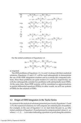
Ordinary And Partial Differential Equation
Routines C C Plus Plus Fortran Java Maple Matlab
download
https://ebookbell.com/product/ordinary-and-partial-differential-
equation-routines-c-c-plus-plus-fortran-java-maple-matlab-2284398
Explore and download more ebooks at ebookbell.com

Here are some recommended products that we believe you will be
interested in. You can click the link to download.
Ordinary And Partial Differential Equation Routines In C C Fortran
Java Maple And Matlab 1st Edition Hj Lee
equation-routines-in-c-c-fortran-java-maple-and-matlab-1st-edition-hj-
lee-1309098
Ordinary And Partial Differential Equations Henner Victor Belozerova
equations-henner-victor-belozerova-5144318
Ordinary And Partial Differential Equations With Special Functions
Fourier Series And Boundary Value Problems 1st Edition Ravi P Agarwal
equations-with-special-functions-fourier-series-and-boundary-value-
problems-1st-edition-ravi-p-agarwal-1007886
Ordinary And Partial Differential Equations An Introduction To
Dynamical Systems John W Cain
equations-an-introduction-to-dynamical-systems-john-w-cain-2341806

Ordinary And Partial Differential Equations An Introduction To
Dynamical Systems Cain Jw
equations-an-introduction-to-dynamical-systems-cain-jw-9973530
Finite Difference Methods For Ordinary And Partial Differential
Equations Steadystate And Timedependent Problems Randall Jleveque
https://ebookbell.com/product/finite-difference-methods-for-ordinary-
and-partial-differential-equations-steadystate-and-timedependent-
problems-randall-jleveque-34998058
Introduction To Numerical Ordinary And Partial Differential Equations
Using Matlab 1st Edition Alexander Stanoyevitch
https://ebookbell.com/product/introduction-to-numerical-ordinary-and-
partial-differential-equations-using-matlab-1st-edition-alexander-
stanoyevitch-4171218
Operator Methods In Ordinary And Partial Differential Equations S
Kovalevsky Symposium University Of Stockholm June 2000 1st Edition
Sergio Albeverio
https://ebookbell.com/product/operator-methods-in-ordinary-and-
partial-differential-equations-s-kovalevsky-symposium-university-of-
stockholm-june-2000-1st-edition-sergio-albeverio-4207004
The Numerical Solution Of Ordinary And Partial Differential Equations
Second Edition Granville Sewellauth
https://ebookbell.com/product/the-numerical-solution-of-ordinary-and-
partial-differential-equations-second-edition-granville-
sewellauth-4309222

CHAPMAN & HALL/CRC
A CRC Press Company
Boca Raton London NewYork Washington, D.C.
Ordinary and Partial Differential
Equation Routines in C, C++,
Fortran,Java®
,Maple®
,andMATLAB®
H.J. Lee and W.E. Schiesser
Copyright 2004 by Chapman & Hall/CRC

Preface
Initial value ordinary differential equations (ODEs) and partial differential
equations (PDEs) are among the most widely used forms of mathematics in
science and engineering. However, insights from ODE/PDE-based models
are realized only when solutions to the equations are produced with accept-
able accuracy and with reasonable effort.
Most ODE/PDE models are complicated enough (e.g., sets of simultane-
ous nonlinear equations) to preclude analytical methods of solution; instead,
numerical methods must be used, which is the central topic of this book.
The calculation of a numerical solution usually requires that well-
established numerical integration algorithms are implemented in quality li-
brary routines. The library routines in turn can be coded (programmed) in a
variety of programming languages. Typically, for a scientist or engineer with
an ODE/PDE- based mathematical model, finding routines written in a famil-
iar language can be a demanding requirement, and perhaps even impossible
(if such routines do not exist).
The purpose of this book, therefore, is to provide a set of ODE/PDE in-
tegration routines written in six widely accepted and used languages. Our
intention is to facilitate ODE/PDE-based analysis by using the library rou-
tines to compute reliable numerical solutions to the ODE/PDE system of
interest.
However, the integration of ODE/PDEs is a large subject, and to keep this
discussion to reasonable length, we have limited the selection of algorithms
and the associated routines. Specifically, we concentrate on explicit (nonstiff)
Runge Kutta (RK) embedded pairs. Within this setting, we have provided
integrators that are both fixed step and variable step; the latter accept a user-
specified error tolerance and attempt to compute a solution to this required
accuracy. The discussion of ODE integration includes truncation error moni-
toring and control, h and p refinement, stability and stiffness, and explicit and
implicit algorithms. Extensions to stiff systems are also discussed and illus-
trated through an ODE application; however, a detailed presentation of stiff
(implicit) algorithms and associated software in six languages was judged
impractical for a book of reasonable length.
Further, we have illustrated the application of the ODE integration routines
to PDEs through the method of lines (MOL). Briefly, the spatial (boundary
value) derivatives of the PDEs are approximated algebraically, typically by
finite differences (FDs); the resulting system of initial-value ODEs is then
solved numerically by one of the ODE routines.

Thus, we have attempted to provide the reader with a set of computational
tools for the convenient solution of ODE/PDE models when programming
in any of the six languages. The discussion is introductory with limited math-
ematical details. Rather, we rely on numerical results to illustrate some basic
mathematical properties, and we avoid detailed mathematical analysis (e.g.,
theorems and proofs), which may not really provide much assistance in the
actual calculation of numerical solutions to ODE/PDE problems.
Instead, we have attempted to provide useful computational tools in the
form of software. The use of the software is illustrated through a small number
of ODE/PDE applications; in each case, the complete code is first presented,
and then its components are discussed in detail, with particular reference
to the concepts of integration, e.g., stability, error monitoring, and control.
Since the algorithms and the associated software have limitations (as do all
algorithms and software), we have tried to point out these limitations, and
make suggestions for additional methods that could be effective.
Also, we have intentionally avoided using features specific to a particular
language, e.g., sparse utilities, object-oriented programming. Rather, we have
emphasized the commonality of the programming in the six languages, and
thereby illustrate how scientific computation can be done in any of the lan-
guages. Of course, language-specific features can be added to the source code
that is provided.
We hope this format will allow the reader to understand the basic elements
of ODE/PDE integration, and then proceed expeditiously to a numerical solu-
tion of the ODE/PDE system of interest. The applications discussed in detail,
two in ODEs and two in PDEs, can be used as a starting point (i.e., as tem-
plates) for the development of a spectrum of new applications.
We welcome comments and questions about how we might be of assis-
tance (directed to wes1@lehigh.edu). Information for acquiring (gratis) all the
source code in this book is available from http://www.lehigh.edu/˜ wes1/
wes1.html. Additional information about the book and software is available
from the CRC Press Web site, http://www.crcpress.com.
Dr. Fred Chapman provided expert assistance with the Maple program-
ming. We note with sadness the passing of Jaeson Lee, father of H. J. Lee,
during the completion of H. J. Lee’s graduate studies at Lehigh University.
H. J. Lee
W. E. Schiesser
Bethlehem, PA

Contents
1 Some Basics of ODE Integration
1.1 General Initial Value ODE Problem
1.2 Origin of ODE Integrators in the Taylor Series
1.3 The Runge Kutta Method
1.4 Accuracy of RK Methods
1.5 Embedded RK Algorithms
1.6 Library ODE Integrators
1.7 Stability of RK Methods
2 Solution of a 1x1 ODE System
2.1 Programming in MATLAB
2.2 Programming in C
2.3 Programming in C++
2.4 Programming in Fortran
2.5 Programming in Java
2.6 Programming in Maple
3 Solution of a 2x2 ODE System
4 Solution of a Linear PDE
5 Solution of a Nonlinear PDE

AppendixA Embedded Runge Kutta Pairs
AppendixB Integrals from ODEs
AppendixC Stiff ODE Integration
C.1 The BDF Formulas Applied to the 2x2 ODE System
C.2 MATLAB Program for the Solution of the
2x2 ODE System
C.3 MATLAB Program for the Solution of the 2x2 ODE System
Using ode23s and ode15s
AppendixD Alternative Forms of ODEs
AppendixE Spatial p Refinement
AppendixF Testing ODE/PDE Codes

1
Some Basics of ODE Integration
The central topic of this book is the programming and use of a set of li-
brary routines for the numerical solution (integration) of systems of initial
value ordinary differential equations (ODEs). We start by reviewing some
of the basic concepts of ODEs, including methods of integration, that are
the mathematical foundation for an understanding of the ODE integration
routines.
1.1 General Initial Value ODE Problem
The general problem for a single initial-value ODE is simply stated as
dy
dt
= f (y, t), y(t0) = y0 (1.1)(1.2)
where
y = dependent variable
t = independent variable
f (y, t) = derivative function
t0 = initial value of the independent variable
y0 = initial value of the dependent variable
Equations 1.1 and 1.2 will be termed a 1x1 problem (one equation in one un-
known). The solution of this 1x1 problem is the dependent variable as a function
of the independent variable, y(t) (this function when substituted into Equations
1.1 and 1.2 satisfies these equations). This solution may be a mathematical
function, termed an analytical solution.

To illustrate these ideas, we consider the 1x1 problem, from Braun1
(which
will be discussed subsequently in more detail)
dy
dt
= λe−αt
y, y(t0) = y0 (1.3)(1.4)
where λ and α are positive constants.
Equation 1.3 is termed a first-order, linear, ordinary differential equation with
variable coefficients. These terms are explained below.
Term Explanation
Differential equation Equation 1.3 has a derivative dy/dt = f (y, t) = λe−αt
y
Ordinary Equation 1.3 has only one independent variable, t, so that
the derivative dy/dt is a total or ordinary derivative
First-order The highest-order derivative is first order (dy/dt is
first order)
Linear y and its derivative dy/dt are to the first power; thus,
Equation 1.3 is also termed first degree (do not confuse
order and degree)
Variable coefficient The coefficient e−αt
is a function of the independent
variable, t (if it were a function of the dependent
variable, y, Equation 1.3 would be nonlinear or not
first degree)
The analytical solution to Equations 1.3 and 1.4 is from Braun:1
y(t) = y0 exp

λ
α
(1 − exp(−αt))

, y(0) = y0 (1.5)
where exp(x) = ex
. Equation 1.5 is easily verified as the solution to Equations
1.3 and 1.4 by substitution in these equations:
Terms in Substitution of Equation 1.5
Equations 1.3 and 1.4 in Equations 1.3 and 1.4
dy
dt
y0 exp

λ
α
(1 − exp(−αt))

λ
α

(−exp(−αt))(−α)
= λy0 exp

λ
α
(1 − exp(−αt))

(exp(−αt))
−λe−αt
y −λe−αt
y0 exp

λ
α
(1 − exp(−αt))

= =
0 0
y(0) y0 exp

λ
α
(1 − exp(−α(0)))

= y0(e0
) = y0
thus confirming Equation 1.5 satisfies Equations 1.3 and 1.4.
Copyright 2004 by Chapman Hall/CRC

As an example of a nxn problem (n ODEs in n unknowns), we will also
subsequently consider in detail the 2x2 system
dy1
dt
= a11 y1 + a12 y2 y1(0) = y10
dy2
dt
= a21 y1 + a22 y2 y2(0) = y20
(1.6)
The solution to Equations 1.6 is again the dependent variables, y1, y2, as a
function of the independent variable, t. Since Equations 1.6 are linear, constant
coefficient ODEs, their solution is easily derived, e.g., by assuming exponential
functions in t or by the Laplace transform. If we assume exponential functions
y1(t) = c1eλt
y2(t) = c2eλt
(1.7)
where c1, c2, and λ are constants to be determined, substitution of Equations
1.7 in Equations 1.6 gives
c1λeλt
= a11c1eλt
+ a12c2eλt
c2λeλt
= a21c1eλt
+ a22c2eλt
Cancellation of eλt
gives a system of algebraic equations (this is the reason
assumingexponentialsolutionsworksinthecaseoflinear,constantcoefficient
ODEs)
c1λ = a11c1 + a12c2
c2λ = a21c1 + a22c2
or
(a11 − λ)c1 + a12c2 = 0
a21c1 + (a22 − λ)c2 = 0
(1.8)
Equations 1.8 are the 2x2 case of the linear algebraic eigenvalue problem
(A − λI)c = 0 (1.9)
where
A =





a11 a12 · · · a1n
a21 a22 · · · a2n
.
.
.
...
.
.
.
an1 an2 · · · ann





I =





1 0 · · · 0
0 1 · · · 0
.
.
.
...
.
.
.
0 0 · · · 1






c =





c1
c2
.
.
.
cn





0 =





0
0
.
.
.
0





n = 2 for Equations 1.8, and we use a bold faced symbol for a matrix or a
vector.
The preceding matrices and vectors are
A nxn coefficient matrix
I nxn identity matrix
c nx1 solution vector
0 nx1 zero vector
The reader should confirm that the matrices and vectors in Equation 1.9 have
the correct dimensions for all of the indicated operations (e.g., matrix addi-
tions, matrix-vector multiples).
Note that Equation 1.9 is a linear, homogeneous algebraic system (homoge-
neous means that the right-hand side (RHS) is the zero vector). Thus, Equation
1.9, or its 2x2 counterpart, Equations 1.8, will have nontrivial solutions (c = 0)
if and only if (iff) the determinant of the coefficient matrix is zero, i.e.,
|A − λI| = 0 (1.10)
Equation 1.10 is the characteristic equation for Equation 1.9 (note that it is a
scalar equation). The values of λ that satisfy Equation 1.10 are the eigenvalues
of Equation 1.9. For the 2x2 problem of Equations 1.8, Equation 1.10 is
a11 − λ a12
a21 a22 − λ
= 0
or
(a11 − λ)(a22 − λ) − a21a12 = 0 (1.11)
Equation 1.11 is the characteristic equation or characteristic polynomial for
Equations 1.8; note that since Equations 1.8 are a 2x2 linear homogeneous
algebraic system, the characteristic equation (Equation 1.11) is a second-order

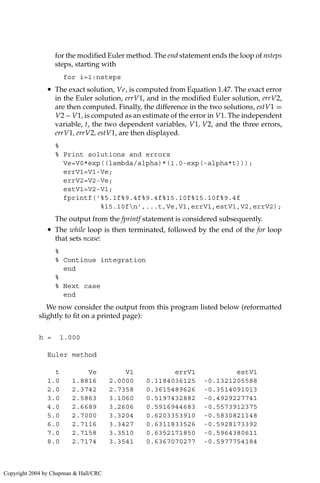
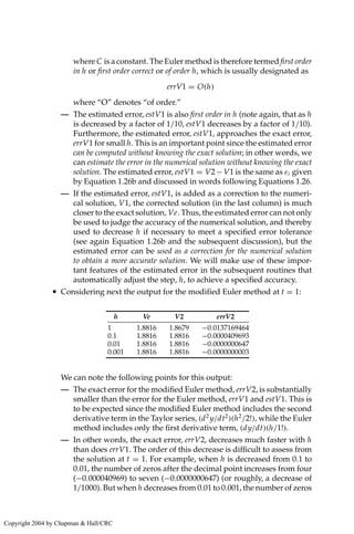
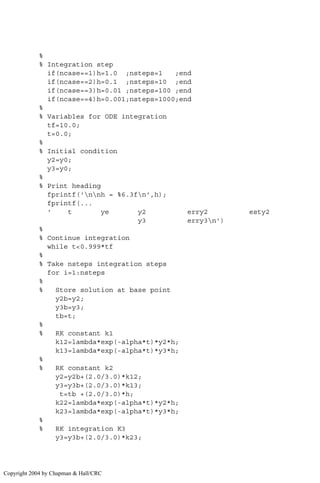
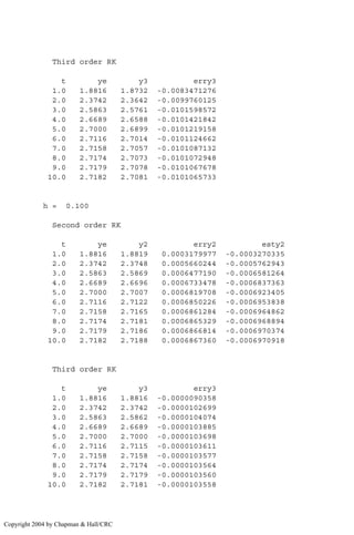
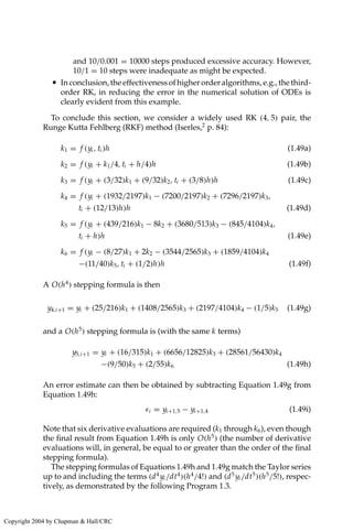
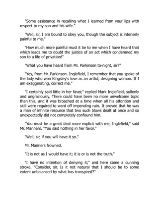
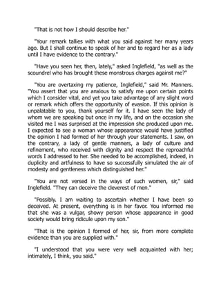
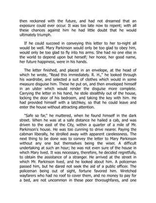
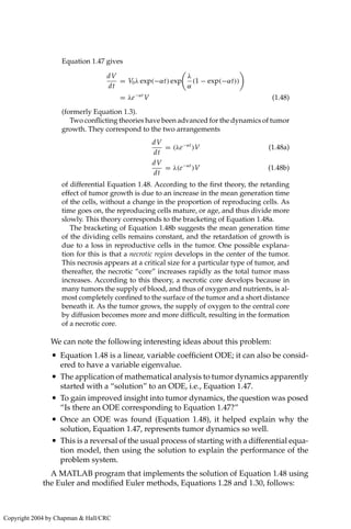
polynomial. Similarly, since Equation 1.9 is a nxn linear homogeneous alge-
braic system, its characteristic equation is a nth-order polynomial.
Equation 1.11 can be factored by the quadratic formula
λ2
− (a11 + a22)λ + a11a22 − a21a12 = 0
λ1, λ2 =
(a11 + a22) ± (a11 + a22)2 − 4(a11a22 − a21a12)
2
(1.12)
Thus, as expected, the 2x2 system of Equations 1.8 has two eigenvalues.
In general, the nxn algebraic system, Equation 1.9, will have n eigenval-
ues, λ1, λ2, . . . , λn (which may be real or complex conjugates, distinct or
repeated).
Since Equations 1.6 are linear constant coefficient ODEs, their general so-
lution will be a linear combination of exponential functions, one for each
eigenvalue
y1 = c11eλ1t
+ c12eλ2t
y2 = c21eλ1t
+ c22eλ2t
(1.13)
Equations 1.13 have four constants which occur in pairs, one pair for each
eigenvalue. Thus, the pair [c11 c21]T
is the eigenvector for eigenvalue λ1 while
[c12 c22]T
is the eigenvector for eigenvalue λ2. In general, the nxn system of
Equation 1.9 will have a nx1 eigenvector for each of its n eigenvalues. Note
that the naming convention for any constant in an eigenvector, ci j , is the
ith constant for the jth eigenvalue. We can restate the two eigenvectors for
Equation 1.13 (or Equations 1.8) as
c11
c21 λ1
,
c12
c22 λ2
(1.14)
Finally, the four constants in eigenvectors (Equations 1.14) are related
through the initial conditions of Equations 1.6 and either of Equations 1.8
y10 = c11eλ10
+ c12eλ20
y20 = c21eλ10
+ c22eλ20
(1.15)
To simplify the analysis somewhat, we consider the special case a11 = a22 =
−a, a21 = a12 = b, where a and b are constants. Then from Equation 1.12,
λ1, λ2 =
−2a ± (2a)2 − 4(a2 − b2)
2
= −a ± b = −(a − b), −(a + b) (1.16)

From the first of Equations 1.8 for λ = λ1
(a11 − λ1)c11 + a12c21 = 0
or
(−a + (a − b))c11 + bc21 = 0
c11 = c21
Similarly, for λ = λ2
(a11 − λ2)c12 + a12c22 = 0
or
(−a + (a + b))c12 + bc22 = 0
c12 = −c22
Substitution of these results in Equations 1.15 gives
y10 = c11 − c22
y20 = c11 + c22
or
c11 =
y10 + y20
2
= c21
c22 =
y20 − y10
2
= −c12
Finally, the solution from Equations 1.13 is
y1 =
y10 + y20
2
eλ1t
−
y20 − y10
2
eλ2t
y2 =
y10 + y20
2
eλ1t
+
y20 − y10
2
eλ2t
(1.17)
Equations 1.17 can easily be checked by substitution in Equations 1.6 (with
a11 = a22 = −a, a21 = a12 = b) and application of the initial conditions at
t = 0:

dy1
dt
λ1
y10 + y20
2
eλ1t
− λ2
y20 − y10
2
eλ2t
= −(a − b)
y10 + y20
2
eλ1t
+ (a + b)
y20 − y10
2
eλ2t
+ay1 +a
y10 + y20
2
eλ1t
−
y20 − y10
2
eλ2t

−by2 −b
y10 + y20
2
eλ1t
+
y20 − y10
2
eλ2t

= =
0 0
dy2
dt
λ1
y10 + y20
2
eλ1t
+ λ2
y20 − y10
2
eλ2t
= −(a − b)
y10 + y20
2
eλ1t
− (a + b)
y20 − y10
2
eλ2t
+ay2 +a
y10 + y20
2
eλ1t
+
y20 − y10
2
eλ2t

−by1 −b
y10 + y20
2
eλ1t
−
y20 − y10
2
eλ2t

= =
0 0
For the initial conditions of Equations 1.6
y10 =
y10 + y20
2
eλ10
−
y20 − y10
2
eλ20
= y10
y20 =
y10 + y20
2
eλ10
+
y20 − y10
2
eλ20
= y20
as required.
The ODE problems of Equations 1.3, 1.4, and 1.6 along with their analytical
solutions, Equations 1.5 and 1.17, will be used subsequently to demonstrate
the use of the ODE integration routines and to evaluate the computed solu-
tions. Since these problems are quite modest (1x1 and 2x2, respectively), we
will also subsequently consider two problems with substantially more ODEs.
At the same time, these ODE systems will be considered as approximations
to partial differential equations (PDEs); in other words, we will use systems
of ODEs for the solution of PDEs.
1.2 Origin of ODE Integrators in the Taylor Series
In contrast to the analytical solutions presented previously (Equations 1.5 and
1.17), the numerical solutions we will compute are ordered pairs of numbers.
For example, in the case of Equation 1.3, we start from the pair (t0, y0) (the
initial condition of Equation 1.3) and proceed to compute paired values (ti , yi )
where i = 1, 2, . . . is an index indicating a position or point along the solution.

Taylor series (Equation 1.18), in this case, to Equation 1.19. In other words, εi
is the truncation error for Euler’s method, Equation 1.19.
We could logically argue that the truncation error could be reduced (for a
given h) by including more terms in the Taylor, e.g., the second derivative
term (d2
yi /dt2
)(h2
/2!). Although this is technically true, there is a practical
problem. For the general ODE, Equation 1.1, we have only the first derivative
available
dyi
dt
= f (yi , ti )
The question then in using the second derivative term of the Taylor series
is “How do we obtain the second derivative, d2
yi /dt2
?”. One answer would
be to differentiate the ODE, i.e.,
d2
y
dt2
=
d
dt

dy
dt

=
d f (y, t)
dt
=
∂ f
∂y
dy
dt
+
∂ f
∂t
=
∂ f
∂y
f +
∂ f
∂t
(1.20)
Then we can substitute Equation 1.20 in Equation 1.18:
yi+1 = yi + fi h +

∂ f
∂y
f +
∂ f
∂t

i
h2
2!
(1.21)
where again subscript “i” means evaluated at point i.
As an example of the application of Equation 1.21, consider the model ODE
dy
dt
= f (y, t) = λy (1.22)
where λ is a constant. Then
fi = λyi

∂ f
∂y
f +
∂ f
∂t

i
= λ (λyi )
(note: ∂ f /∂t = 0 since f = λy does not depend on t) and substitution in
Equation 1.21 gives
yi+1 = yi + λyi h + λ (λyi )
h2
2!
= yi (1 + λh + (λh)2
/2!)
yi (1+λh+(λh)2
/2!) is the Taylor series of yi eλh
up to and including the h2
term,
but yi eλh
is the analytical solution to Equation 1.22 with the initial condition
y(ti ) = yi for the integration step, h = ti+1 − ti . Thus, as stated previously,
Equation 1.21 fits the Taylor series of the analytical solution to Equation 1.22
up to and including the (d2
yi /dt2
)(h2
/2!) term.
Of course, we could, in principle, continue this process of including ad-
ditional terms in the Taylor series, e.g., using the derivative of the second

derivative to arrive at the third derivative, etc. Clearly, however, the method
quickly becomes cumbersome (and this is for only one ODE, Equation 1.1).
Application of this Taylor series method to systems of ODEs involves a lot of
differentiation. (Would we want to apply it to a system of 100 or 1000 ODEs?
We think not.)
Ideally, we would like to have a higher-order ODE integration method
(higher than the first-order Euler method) without having to take derivatives
of the ODEs. Although this may seem like an impossibility, it can in fact be
done by the Runge Kutta (RK) method. In other words, the RK method can be
used to fit the numerical ODE solution exactly to an arbitrary number of terms
in the underlying Taylor series without having to differentiate the ODE. We will
investigate the RK method, which is the basis for the ODE integration routines
described in this book.
The other important characteristic of a numerical integration algorithm (in
addition to not having to differentiate the ODE) is a way of estimating the
truncation error, ε, so that the integration step, h, can be adjusted to achieve a
solution with a prescribed accuracy. This may also seem like an impossibility
since it would appear that in order to compute ε we need to know the exact
(analytical)solution.Butiftheexactsolutionisknown,therewouldbenoneed
to calculate the numerical solution. The answer to this apparent contradiction
is the fact that we will calculate an estimate of the truncation error (and not the
exact truncation error which would imply that we know the exact solution). To
see how this might be done, consider computing a truncation error estimate
for the Euler method. Again, we return to the Taylor series (which is the
mathematical tool for most of the numerical analysis of ODE integration).
Now we will expand the first derivative dy/dt
dyi+1
dt
=
dyi
dt
+
d2
yi
dt2
h
1!
+ · · · (1.23)
d2
yi /dt2
is the second derivative we require in Equation 1.18. If the Taylor
series in Equation 1.23 is truncated after the h term, we can solve for this
second derivative
d2
yi
dt2
=
dyi+1
dt
−
dyi
dt
h
(1.24)
Equation 1.24 seems logical, i.e., the second derivative is a finite difference
(FD) approximation of the first derivative. Note that Equation 1.24 has the im-
portant property that we can compute the second derivative without having
to differentiate the ODE; rather, all we have to do is use the ODE twice, at
grid points i and i + 1. Thus, the previous differentiation of Equation 1.20 is
avoided. However, note also that Equation 1.24 gives only an approximation
for the second derivative since it results from truncating the Taylor series of
Equation 1.23. Fortunately, the approximation of Equation 1.24 will generally

is too large and causes the large overshoot of the numerical solution above
the exact solution (and thus, a relatively large value of εi ), the averaging of
the derivatives at i and i + 1 in Figure 1.2 reduces this overshoot (and the
truncation error is reduced from ε
p
i to εc
i ).
Equation 1.25 can be rearranged into a more useful form. If we assume
that the truncation error of Euler’s method, εi , is due mainly to the second
derivative term (d2
yi /dt2
)(h2
/2!) of Equation 1.18 (which will be the case if
the higher-order terms in Equation 1.18 are negligibly small), then
εi =
d2
yi
dt2
h2
2!
=
dyi+1
dt
−
dyi
dt
h
h2
2!
=

dyi+1
dt
−
dyi
dt

h
2!
and Equation 1.25 can be written as a two-step algorithm:
y
p
i+1 = yi +
dyi
dt
h (1.26a)
εi =

dy
p
i+1
dt
−
dyi
dt

h
2!
(1.26b)
yc
i+1 = yi +
dyi
dt
h + εi = y
p
i+1 + εi (1.26c)
With a little algebra, we can easily show that yi+1 of Equation 1.25 and y
p
i+1
of Equation 1.26c are the same. While Equation 1.25 and Equations 1.26c are
mathematically equivalent, Equations 1.26 have an advantage when used in
a computer program. Specifically, an algorithm that automatically adjusts h
to achieve a prescribed accuracy, tol, can be programmed in the following
steps:
1. Compute y
p
i+1 by the Euler method, Equation 1.26a. The superscript p
in this case denotes a predicted value.
2. Compute the estimated error, εi , from Equation 1.26b. Note that
dy
p
i+1/dt = f (y
p
i+1, ti+1), where ti+1 = ti + h.
3. Pose the question is εi tol? If no, reduce h and return to 1. If yes,
continue to 4.
4. Add εi from 3 to y
p
i+1 to obtain yc
i+1 according to Equation 1.26c. The
superscript c denotes a corrected value.
5. Increment i, advance ti to ti+1 by adding h, go to 1. to take the next step
along the solution.
The algorithm of Equations 1.26 is termed a predictor-corrector method, which
we will subsequently discuss in terms of a computer program.
To conclude this introductory discussion of integration algorithms, we in-
troduce the RK notation. If we define k1 and k2 (termed Runge Kutta constants

although they are not constant, but rather, vary along the solution) as
k1 = f (yi , ti )h (1.27a)
k2 = f (yi + k1, ti + h)h (1.27b)
the Euler method of Equation 1.19 can be written as (keep in mind dy/dt =
f (y, t))
yi+1 = yi + k1 (1.28)
and the modified Euler method of Equation 1.25 can be written
yi+1 = yi +
k1 + k2
2
(1.29)
(the reader should confirm that Equation 1.25 and Equation 1.29 are the same).
Also, the modified Euler method written in terms of an explicit error esti-
mate, Equations 1.26, can be conveniently written in RK notation:
y
p
i+1 = yi + k1 (1.30a)
εi =
(k2 − k1)
2
(1.30b)
yc
i+1 = yi + k1 +
(k2 − k1)
2
= yi +
(k1 + k2)
2
(1.30c)
However, the RK method is much more than just a convenient system of
notation.Asstatedearlier,itisamethodforfittingtheunderlyingTaylorseries
of the ODE solution to any number of terms without having to differentiate
the ODE (it requires only the first derivative in dy/dt = f (y, t) as we observe
in Equations 1.29 and 1.30). We next explore this important feature of the RK
method, which is the mathematical foundation of the ODE integrators to be
discussed subsequently.
1.3 The Runge Kutta Method
The RK method consists of a series of algorithms of increasing order. There
is only one first order RK method, the Euler method, which fits the underlying
Taylor series of the solution up to and including the first derivative term, as
indicated by Equation 1.19.
The second-order RK method is actually a family of second-order methods;
a particular member of this family is selected by choosing an arbitrary con-
stant in the general second-order RK formulas. The origin of these formulas is

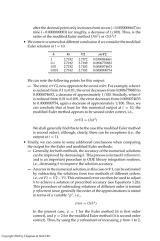
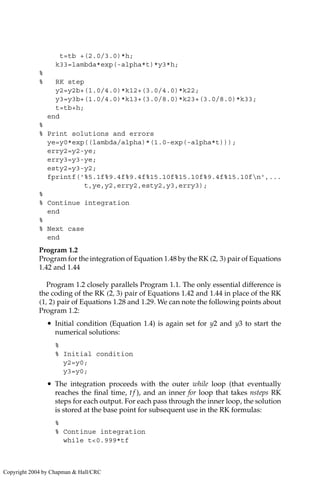
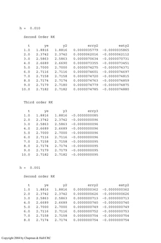
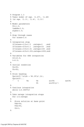
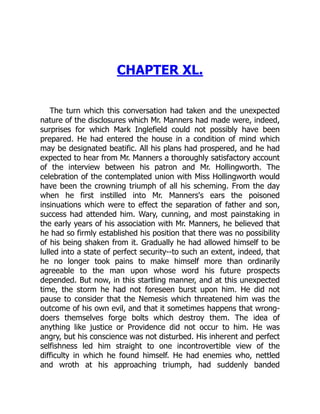
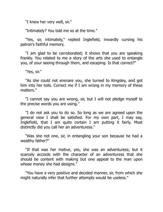
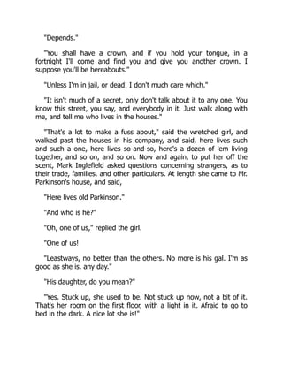
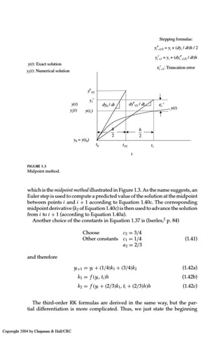
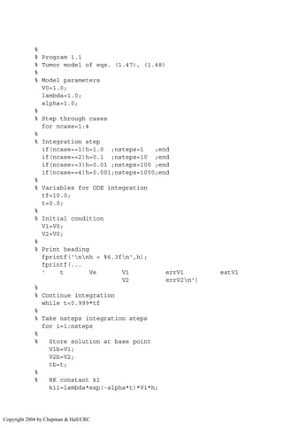
illustrated by the following development (based on the idea that the second-
order RK method fits the Taylor series up to and including the second deriva-
tive term, (d2
yi /dt2
)(h2
/2!)).
We start the analysis with a general RK stepping formula of the form
yi+1 = yi + c1k1 + c2k2 (1.31a)
where k1 and k2 are RK “constants” of the form
k1 = f (yi , ti )h (1.31b)
k2 = f (yi + a2k1(yi , ti ), ti + a2h)h = f (yi + a2 f (yi , ti )h, ti + a2h)h (1.31c)
and c1, c2 and a2 are constants to be determined.
If k2 from Equation 1.31c is expanded in a Taylor series in two variables,
k2 = f (yi + a2 f (yi , ti )h, ti + a2h)h
=

f (yi , ti ) + fy(yi , ti )a2 f (yi , ti )h + ft(yi , ti )a2h

h + O(h3
) (1.32)
Substituting Equations 1.31b and 1.32 in Equation 1.31a gives
yi+1 = yi + c1 f (yi , ti )h + c2[ f (yi , ti ) + fy(yi , ti )a2 f (yi , ti )h
+ ft(yi , ti )a2h]h + O(h3
)
= yi + (c1 + c2) f (yi , ti )h + c2[ fy(yi , ti )a2 f (yi , ti )
+ ft(yi , ti )a2]h2
+ O(h3
) (1.33)
Note that Equation 1.33 is a polynomial in increasing powers of h; i.e., it has
the form of a Taylor series. Thus, if we expand yi+1 in a Taylor series around
yi , we will obtain a polynomial of the same form, i.e., in increasing powers
of h
yi+1 = yi +
dyi
dt
h +
d2
yi
dt2
h2
2!
+ O(h3
)
= yi + f (yi , ti )h +
d f (yi , ti )
dt
h2
2!
+ O(h3
) (1.34)
where we have used dyi /dt = f (yi , ti ), i.e., the ODE we wish to integrate nu-
merically. To match Equations 1.33 and 1.34, term-by-term (with like powers
of h), we need to have [d f (yi , ti )/dt](h2
/2!) in Equation 1.34 in the form of
fy(yi , ti )a2 f (yi , ti ) + ft(yi , ti )a2 in Equation 1.33.
If chain-rule differentiation is applied to d f (yi , ti )/dt
d f (yi , ti )
dt
= fy(yi , ti )
dyi
dt
+ ft(yi , ti ) = fy(yi , ti ) f (yi , ti ) + ft(yi , ti ) (1.35)

Substitution of Equation 1.35 in Equation 1.34 gives
yi+1 = yi + f (yi , ti )h +

fy(yi , ti ) f (yi , ti ) + ft(yi , ti )
h2
2!
+ O(h3
) (1.36)
We can now equate coefficients of like powers of h in Equations 1.33 and 1.36
Power of h Equation 1.33 Equation 1.36
h0
yi yi
h1
(c1 + c2) f (yi , ti ) f (yi , ti )
h2
c2

fy(yi , ti )a2 f (yi , ti ) + ft(yi , ti )a2

fy(yi , ti ) f (yi , ti ) + ft(yi , ti )
1
2!
Thus, we conclude
c1 + c2 = 1
c2a2 = 1/2
(1.37)
This is a system of two equations in three unknowns or constants (c1, c2, a2);
thus, one constant can be selected arbitrarily (there are actually an infinite
number of second-order RK methods, depending on the arbitrary choice of
one of the constants in Equations 1.37). Here is one choice:
Choose c2 = 1/2
Other constants c1 = 1/2
a2 = 1
(1.38)
and the resulting second-order RK method is
yi+1 = yi + c1k1 + c2k2 = yi +
k1 + k2
2
k1 = f (yi , ti )h
k2 = f (yi + a2k1(yi , ti ), ti + a2h)h = f (yi + f (yi , ti )h, ti + h)h
which is the modified Euler method, Equations 1.27, 1.28, and 1.29.
For the choice
Choose c2 = 1
Other constants c1 = 0
a2 = 1/2
(1.39)
the resulting second-order RK method is
yi+1 = yi + c1k1 + c2k2 = yi + k2 (1.40a)
k1 = f (yi , ti )h (1.40b)
k2 = f (yi + a2k1(yi , ti ), ti + a2h)h
= f (yi + (1/2) f (yi , ti )h, ti + (1/2)h)h
= f (yi + (1/2)k1, ti + (1/2)h)h (1.40c)

equations and the final result (Iserles,2
p. 40). The third order stepping for-
mula is
yi+1 = yi + c1k1 + c2k2 + c3k3 (1.43a)
The RK constants are
k1 = f (yi , ti )h (1.43b)
k2 = f (yi + a2k1, ti + a2h)h (1.43c)
k3 = f (yi + b3k1 + (a3 − b3)k2, ti + a3h)h (1.43d)
Four algebraic equations define the six constants c1, c2, c3, a2, a3, b3 (ob-
tained by matching the stepping formula, Equation 1.43a, with the Taylor
series up to and including the term (d3
yi /dt3
)(h3
/3!)
c1 + c2 + c3 = 1 (1.43e)
c2a2 + c3a3 = 1/2 (1.43f)
c2a2
2 + c3a2
3 = 1/3 (1.43g)
c3(a3 − b3)a2 = 1/6 (1.43h)
To illustrate the use of Equations 1.43e to 1.43h, we can take c2 = c3 = 3
8
,
and from Equation 1.43e, c1 = 1 − 3
8
− 3
8
= 2
8
. From Equation 1.43f
(3/8)a2 + (3/8)a3 = 1/2
or a2 = 4
3
− a3. From Equation 1.43g,
(3/8)(4/3 − a3)2
+ (3/8)a2
3 = 1/3
or a3 = 2
3
(by the quadratic formula). Thus, a2 = 4
3
− 2
3
= 2
3
, and from Equation
1.43h,
(3/8)(2/3 − b3)2/3 = 1/6
or b3 = 0.
This particular third-order Nystrom method (Iserles,2
p. 40) is therefore
yi+1 = yi + (2/8)k1 + (3/8)k2 + (3/8)k3 (1.44a)
k1 = f (yi , ti )h (1.44b)
k2 = f (yi + (2/3)k1, ti + (2/3)h)h (1.44c)
k3 = f (yi + (2/3)k2, ti + (2/3)h)h (1.44d)
We next consider some MATLAB code which implements the Euler method
of Equation 1.28, the modified Euler method of Equations 1.30, the second-
order RK of Equations 1.42, and the third-order RK of Equations 1.44.

The objective is to investigate the accuracy of these RK methods in computing
solutions to an ODE test problem.
1.4 Accuracy of RK Methods
We start with the numerical solution of a single ODE, Equation 1.3, subject
to initial condition Equation 1.4, by the Euler and modified Euler methods,
Equation 1.28 and Equations 1.30. The analytical solution, Equation 1.5, can
be used to calculate the exact errors in the numerical solutions.
Equation 1.3 models the growth of tumors, and this important application
is first described in the words of Braun1
(the dependent variable in Equation
1.3 is changed from “y” to “V” corresponding to Braun’s notation where V
denotes tumor volume).
It has been observed experimentally that “free living” dividing cells,
such as bacteria cells, grow at a rate proportional to the volume of the
dividing cells at that moment. Let V(t) denote the volume of the dividing
cells at time t. Then,
dV
dt
= λV (1.45)
for some positive constant λ. The solution of Equation 1.45 is
V(t) = V0eλ(t−t0)
(1.46)
where V0 is the volume of dividing cells at the initial time t0. Thus, free
living dividing cells grow exponentially with time. One important conse-
quence of Equation 1.46 is that the volume of the cells keeps doubling
every time interval of length ln 2/λ.
On the other hand, solid tumors do not grow exponentially with time.
As the tumor becomes larger, the doubling time of the total tumor vol-
ume continuously increases. Various researchers have shown that the data
for many solid tumors is fitted remarkably well, over almost a 1000-fold
increase in tumor volume, by the equation (previously Equation 1.5)
V(t) = V0 exp

λ
α
(1 − exp(−αt))

(1.47)
where exp(x) = ex
, and λ and α are positive constants.
Equation 1.47 is usually referred to as a Gompertzjan relation. It says
that the tumor grows more and more slowly with the passage of time,
and that it ultimately approaches the limiting volume V0eλ/α
. Medical
researchers have long been concerned with explaining this deviation from
simple exponential growth. A great deal of insight into this problem can be
gained by finding a differential equation satisfied by V(t). Differentiating

Equation 1.47 gives
dV
dt
= V0λ exp(−αt) exp

λ
α
(1 − exp(−αt))

= λe−αt
V (1.48)
(formerly Equation 1.3).
Two conflicting theories have been advanced for the dynamics of tumor
growth. They correspond to the two arrangements
dV
dt
= (λe−αt
)V (1.48a)
dV
dt
= λ(e−αt
)V (1.48b)
of differential Equation 1.48. According to the first theory, the retarding
effect of tumor growth is due to an increase in the mean generation time
of the cells, without a change in the proportion of reproducing cells. As
time goes on, the reproducing cells mature, or age, and thus divide more
slowly. This theory corresponds to the bracketing of Equation 1.48a.
The bracketing of Equation 1.48b suggests the mean generation time
of the dividing cells remains constant, and the retardation of growth is
due to a loss in reproductive cells in the tumor. One possible explana-
tion for this is that a necrotic region develops in the center of the tumor.
This necrosis appears at a critical size for a particular type of tumor, and
thereafter, the necrotic “core” increases rapidly as the total tumor mass
increases. According to this theory, a necrotic core develops because in
many tumors the supply of blood, and thus of oxygen and nutrients, is al-
most completely confined to the surface of the tumor and a short distance
beneath it. As the tumor grows, the supply of oxygen to the central core
by diffusion becomes more and more difficult, resulting in the formation
of a necrotic core.
We can note the following interesting ideas about this problem:
• Equation 1.48 is a linear, variable coefficient ODE; it can also be consid-
ered to have a variable eigenvalue.
• The application of mathematical analysis to tumor dynamics apparently
started with a “solution” to an ODE, i.e., Equation 1.47.
• To gain improved insight into tumor dynamics, the question was posed
“Is there an ODE corresponding to Equation 1.47?”
• Once an ODE was found (Equation 1.48), it helped explain why the
solution, Equation 1.47, represents tumor dynamics so well.
• This is a reversal of the usual process of starting with a differential equa-
tion model, then using the solution to explain the performance of the
problem system.
A MATLAB program that implements the solution of Equation 1.48 using
the Euler and modified Euler methods, Equations 1.28 and 1.30, follows:

%
% Program 1.1
% Tumor model of eqs. (1.47), (1.48)
%
% Model parameters
V0=1.0;
lambda=1.0;
alpha=1.0;
%
% Step through cases
for ncase=1:4
%
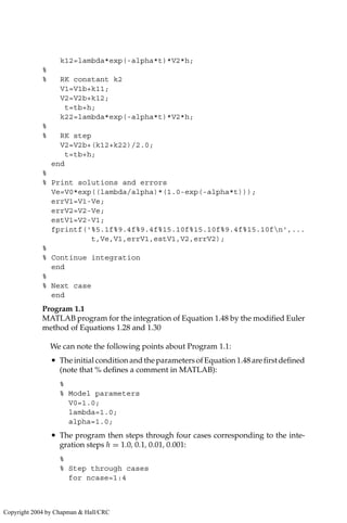
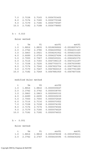
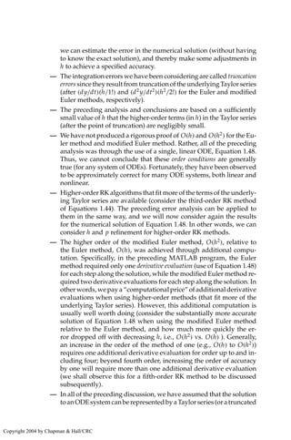
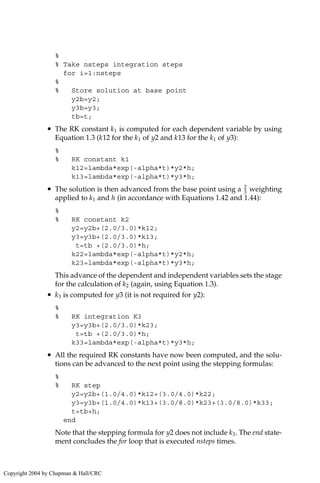
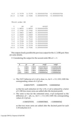
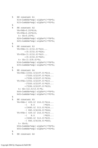
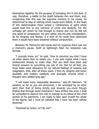
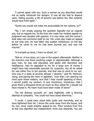
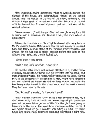
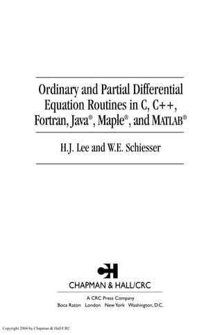
% Integration step
if(ncase==1)h=1.0 ;nsteps=1 ;end
if(ncase==4)h=0.001;nsteps=1000;end
%
% Variables for ODE integration
tf=10.0;
t=0.0;
%
% Initial condition
V1=V0;
V2=V0;
%
% Print heading
fprintf('nnh = %6.3fn',h);
fprintf(...
' t Ve V1 errV1 estV1
V2 errV2n')
%
% Continue integration
while t0.999*tf
%
% Take nsteps integration steps
for i=1:nsteps
%
% Store solution at base point
V1b=V1;
V2b=V2;
tb=t;
%
% RK constant k1
k11=lambda*exp(-alpha*t)*V1*h;

%
% RK constant k2
V1=V1b+k11;
V2=V2b+k12;
t=tb+h;
%
% RK step
V2=V2b+(k12+k22)/2.0;
t=tb+h;
end
%
% Print solutions and errors
Ve=V0*exp((lambda/alpha)*(1.0-exp(-alpha*t)));
errV1=V1-Ve;
errV2=V2-Ve;
estV1=V2-V1;
fprintf('%5.1f%9.4f%9.4f%15.10f%15.10f%9.4f%15.10fn',...
t,Ve,V1,errV1,estV1,V2,errV2);
%
end
%
% Next case
end
Program 1.1
MATLAB program for the integration of Equation 1.48 by the modified Euler
method of Equations 1.28 and 1.30
We can note the following points about Program 1.1:
• The initial condition and the parameters of Equation 1.48 are first defined
(note that % defines a comment in MATLAB):
%
% Model parameters
V0=1.0;
lambda=1.0;
alpha=1.0;
• The program then steps through four cases corresponding to the inte-
gration steps h = 1.0, 0.1, 0.01, 0.001:
%
for ncase=1:4

%
% Integration step
For each h, the corresponding number of integration steps is nsteps.
Thus, the product (h)(nsteps) = 1 unit in t for each output from the
program; i.e., the output from the program is at t = 0, 1, 2, . . . , 10.
• For each case, the initial and final values of t are defined, i.e., t = 0, tf =
10, and the initial condition, V(0) = V0 is set to start the solution:
%
tf=10.0;
t=0.0;
%
% Initial condition
V1=V0;
V2=V0;
Two initial conditions are set, one for the Euler solution, computed as
V1, and one for the modified Euler solution, V2 (subsequently, we will
program the solution vector, in this case [V1 V2]T
, as a one-dimensional
(1D) array).
• A heading indicating the integration step, h, and the two numerical
solutions is then displayed. “. . . ” indicates a line is to be continued on
the next line. (Note: . . . does not work in a character string delineated by
single quotes, so the character string in the second fprintf statement has
been placed on two lines in order to fit within the available page width;
to execute this program, the character string should be returned to one
line.)
%
% Print heading
fprintf(...
V2 errV2n')
• Awhileloopthencomputesthesolutionuntilthefinaltime,tf ,isreached:
%
while t0.999*tf

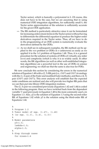
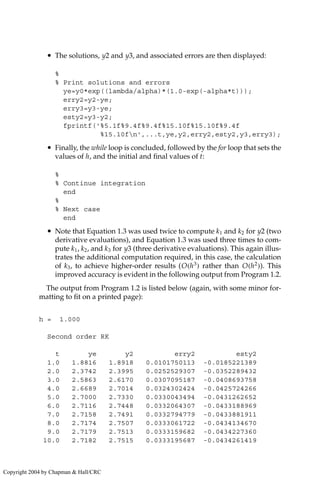
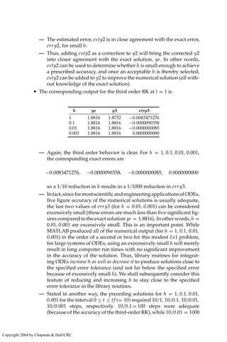
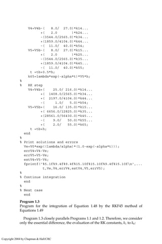
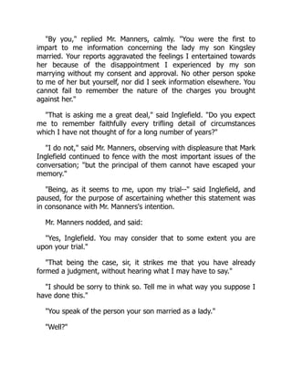
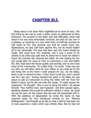
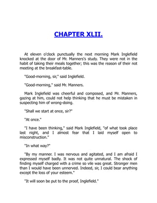
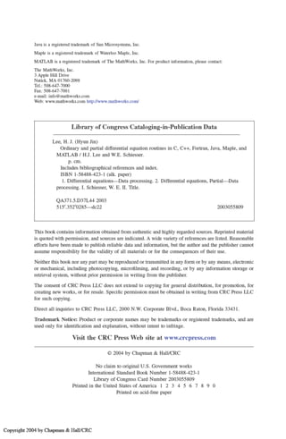
Of course, at the beginning of the execution, t = 0 so the while loop
continues.
• nsteps Euler and modified Euler steps are then taken:
%
for i=1:nsteps
%
V1b=V1;
V2b=V2;
tb=t;
At each point along the solution (point i), the solution is stored for sub-
sequent use in the numerical integration.
• The first RK constant, k1, is then computed for each dependent variable
in [V1 V2)]T
according to Equation 1.27a:
%
% RK constant k1
Note that we have used the RHS of the ODE, Equation 1.48, in computing
k1. k11 is k1 for V1, and k12 is k1 for V2. Subsequently, the RK constants
will be programmed as 1D arrays, e.g., [k1(1) k1(2)]T
.
• The solution is then advanced from the base point according to Equation
1.28:
%
% RK constant k2
V1=V1b+k11;
V2=V2b+k12;
t=tb+h;
The second RK constant, k2 for V2, is then computed according to Equa-
tion 1.27b. At the same time, the independent variable, t, is advanced.
• ThemodifiedEulersolution, V2,isthencomputedaccordingtoEquation
1.29:
%
% RK step
V2=V2b+(k12+k22)/2.0;
t=tb+h;
end
The advance of the independent variable, t, was done previously and is
therefore redundant; it is done again just to emphasize the advance in t

for the modified Euler method. The end statement ends the loop of nsteps
steps, starting with
for i=1:nsteps
• The exact solution, Ve, is computed from Equation 1.47. The exact error
in the Euler solution, errV1, and in the modified Euler solution, errV2,
are then computed. Finally, the difference in the two solutions, estV1 =
V2− V1, is computed as an estimate of the error in V1. The independent
variable, t, the two dependent variables, V1, V2, and the three errors,
errV1, errV2, estV1, are then displayed.
%
errV1=V1-Ve;
errV2=V2-Ve;
estV1=V2-V1;
fprintf('%5.1f%9.4f%9.4f%15.10f%15.10f%9.4f
%15.10fn',...t,Ve,V1,errV1,estV1,V2,errV2);
The output from the fprintf statement is considered subsequently.
• The while loop is then terminated, followed by the end of the for loop
that sets ncase:
%
end
%
% Next case
end
We now consider the output from this program listed below (reformatted
slightly to fit on a printed page):
h = 1.000
Euler method
t Ve V1 errV1 estV1
1.0 1.8816 2.0000 0.1184036125 -0.1321205588
2.0 2.3742 2.7358 0.3615489626 -0.3514091013
3.0 2.5863 3.1060 0.5197432882 -0.4929227741
4.0 2.6689 3.2606 0.5916944683 -0.5573912375
5.0 2.7000 3.3204 0.6203353910 -0.5830821148
6.0 2.7116 3.3427 0.6311833526 -0.5928173392
7.0 2.7158 3.3510 0.6352171850 -0.5964380611
8.0 2.7174 3.3541 0.6367070277 -0.5977754184

9.0 2.7179 3.3552 0.6372559081 -0.5982681335
10.0 2.7182 3.3556 0.6374579380 -0.5984494919
modified Euler method
t Ve V2 errV2
1.0 1.8816 1.8679 -0.0137169464
2.0 2.3742 2.3843 0.0101398613
3.0 2.5863 2.6131 0.0268205142
4.0 2.6689 2.7033 0.0343032307
5.0 2.7000 2.7373 0.0372532762
6.0 2.7116 2.7499 0.0383660134
7.0 2.7158 2.7546 0.0387791239
8.0 2.7174 2.7563 0.0389316092
9.0 2.7179 2.7569 0.0389877746
10.0 2.7182 2.7572 0.0390084461
h = 0.100
Euler method
t Ve V1 errV1 estV1
1.0 1.8816 1.8994 0.0178364041 -0.0178773733
2.0 2.3742 2.4175 0.0433341041 -0.0430037365
3.0 2.5863 2.6438 0.0575343031 -0.0569959440
4.0 2.6689 2.7325 0.0635808894 -0.0629558472
5.0 2.7000 2.7660 0.0659265619 -0.0652682467
6.0 2.7116 2.7784 0.0668064211 -0.0661356782
7.0 2.7158 2.7829 0.0671324218 -0.0664570816
8.0 2.7174 2.7846 0.0672526658 -0.0665756310
9.0 2.7179 2.7852 0.0672969439 -0.0666192852
10.0 2.7182 2.7855 0.0673132386 -0.0666353503
t Ve V2 errV2
1.0 1.8816 1.8816 -0.0000409693
2.0 2.3742 2.3745 0.0003303677
3.0 2.5863 2.5868 0.0005383591
4.0 2.6689 2.6696 0.0006250422
5.0 2.7000 2.7007 0.0006583152
6.0 2.7116 2.7122 0.0006707429

7.0 2.7158 2.7165 0.0006753402
8.0 2.7174 2.7180 0.0006770348
9.0 2.7179 2.7186 0.0006776587
10.0 2.7182 2.7188 0.0006778883
h = 0.010
Euler method
t Ve V1 errV1 estV1
1.0 1.8816 1.8835 0.0018696826 -0.0018697473
2.0 2.3742 2.3786 0.0044269942 -0.0044231149
3.0 2.5863 2.5921 0.0058291952 -0.0058231620
4.0 2.6689 2.6754 0.0064227494 -0.0064158254
5.0 2.7000 2.7067 0.0066525021 -0.0066452372
6.0 2.7116 2.7183 0.0067386119 -0.0067312197
7.0 2.7158 2.7226 0.0067705073 -0.0067630680
8.0 2.7174 2.7242 0.0067822704 -0.0067748139
9.0 2.7179 2.7247 0.0067866019 -0.0067791389
10.0 2.7182 2.7249 0.0067881959 -0.0067807306
t Ve V2 errV2
1.0 1.8816 1.8816 -0.0000000647
2.0 2.3742 2.3742 0.0000038793
3.0 2.5863 2.5863 0.0000060332
4.0 2.6689 2.6690 0.0000069239
5.0 2.7000 2.7000 0.0000072649
6.0 2.7116 2.7116 0.0000073922
7.0 2.7158 2.7158 0.0000074392
8.0 2.7174 2.7174 0.0000074566
9.0 2.7179 2.7180 0.0000074629
10.0 2.7182 2.7182 0.0000074653
h = 0.001
Euler method
t Ve V1 errV1 estV1
1.0 1.8816 1.8818 0.0001878608 -0.0001878611
2.0 2.3742 2.3747 0.0004436596 -0.0004436202

3.0 2.5863 2.5868 0.0005836997 -0.0005836386
4.0 2.6689 2.6696 0.0006429444 -0.0006428744
5.0 2.7000 2.7007 0.0006658719 -0.0006657985
6.0 2.7116 2.7122 0.0006744643 -0.0006743896
7.0 2.7158 2.7165 0.0006776469 -0.0006775717
8.0 2.7174 2.7180 0.0006788206 -0.0006787453
9.0 2.7179 2.7186 0.0006792528 -0.0006791774
10.0 2.7182 2.7188 0.0006794118 -0.0006793364
t Ve V2 errV2
1.0 1.8816 1.8816 -0.0000000003
2.0 2.3742 2.3742 0.0000000394
3.0 2.5863 2.5863 0.0000000610
4.0 2.6689 2.6689 0.0000000700
5.0 2.7000 2.7000 0.0000000734
6.0 2.7116 2.7116 0.0000000747
7.0 2.7158 2.7158 0.0000000751
8.0 2.7174 2.7174 0.0000000753
9.0 2.7179 2.7179 0.0000000754
10.0 2.7182 2.7182 0.0000000754
We can note the following points about this output:
• Considering first the output for the Euler method at t = 1:
h Ve V1 errV1 estV1 V1 + estV1
1 1.8816 2.0000 0.1184036125 −0.1321205588 1.8679
0.1 1.8816 1.8994 0.0178364041 −0.0178773733 1.8815
0.01 1.8816 1.8835 0.0018696826 −0.0018697473 1.8816
0.001 1.8816 1.8818 0.0001878608 −0.0001878611 1.8816
We can note the following points for this output:
— The exact error, errV1, decreases linearly with integration step, h.
For example, when h is decreased from 0.01 to 0.001, errV1 decreases
from0.0018696826to0.0001878608.Roughlyspeaking,asthedecimal
point in h moves one place, the decimal point in errV1 moves one
place. However, this is true only when h becomes small (so that
higher-order terms in the underlying Taylor series become negligibly
small).
— Thus, the error in the Euler method is proportional to h
errV1 = Ch1

where C is a constant. The Euler method is therefore termed first order
in h or first order correct or of order h, which is usually designated as
errV1 = O(h)
where “O” denotes “of order.”
— The estimated error, estV1 is also first order in h (note again, that as h
is decreased by a factor of 1/10, estV1 decreases by a factor of 1/10).
Furthermore, the estimated error, estV1, approaches the exact error,
errV1 for small h. This is an important point since the estimated error
can be computed without knowing the exact solution; in other words, we
can estimate the error in the numerical solution without knowing the exact
solution. The estimated error, estV1 = V2− V1 is the same as εi given
by Equation 1.26b and discussed in words following Equations 1.26.
— If the estimated error, estV1, is added as a correction to the numeri-
cal solution, V1, the corrected solution (in the last column) is much
closer to the exact solution, Ve. Thus, the estimated error can not only
be used to judge the accuracy of the numerical solution, and thereby
used to decrease h if necessary to meet a specified error tolerance
(see again Equation 1.26b and the subsequent discussion), but the
estimated error can be used as a correction for the numerical solution
to obtain a more accurate solution. We will make use of these impor-
tant features of the estimated error in the subsequent routines that
automatically adjust the step, h, to achieve a specified accuracy.
• Considering next the output for the modified Euler method at t = 1:
h Ve V2 errV2
1 1.8816 1.8679 −0.0137169464
0.1 1.8816 1.8816 −0.0000409693
0.01 1.8816 1.8816 −0.0000000647
0.001 1.8816 1.8816 −0.0000000003
— The exact error for the modified Euler method, errV2, is substantially
smaller than the error for the Euler method, errV1 and estV1. This is
to be expected since the modified Euler method includes the second
derivative term in the Taylor series, (d2
y/dt2
)(h2
/2!), while the Euler
method includes only the first derivative term, (dy/dt)(h/1!).
— In other words, the exact error, errV2, decreases much faster with h
than does errV1. The order of this decrease is difficult to assess from
the solution at t = 1. For example, when h is decreased from 0.1 to
0.01, the number of zeros after the decimal point increases from four
(−0.000040969) to seven (−0.0000000647) (or roughly, a decrease of
1/1000). But when h decreases from 0.01 to 0.001, the number of zeros

after the decimal point only increases from seven (−0.0000000647) to
nine (−0.0000000003) (or roughly, a decrease of 1/100). Thus, is the
order of the modified Euler method O(h2
) or O(h3
)?
• We come to a somewhat different conclusion if we consider the modified
Euler solution at t = 10:
h Ve V2 errV2
1 2.7182 2.7572 0.0390084461
0.1 2.7182 2.7188 0.0006778883
0.01 2.7182 2.7182 0.0000074653
0.001 2.7182 2.7182 0.0000000754
— The error, errV2, now appears to be second order. For example, when h
is reduced from 0.1 to 0.01, the error decreases from 0.0006778883 to
0.0000074653, a decrease of approximately 1/100. Similarly, when h
is reduced from 0.01 to 0.001, the error decreases from 0.0000074653
to 0.0000000754, again a decrease of approximately 1/100. Thus, we
can conclude that at least for this numerical output at t = 10, the
modified Euler method appears to be second order correct, i.e.,
errV2 = O(h2
)
We shall generally find this to be the case (the modified Euler method
is second order), although, clearly, there can be exceptions (i.e., the
output at t = 1).
• Finally, we can come to some additional conclusions when comparing
the output for the Euler and modified Euler methods:
— Generally, for both methods, the accuracy of the numerical solutions
can be improved by decreasing h. This process is termed h refinement,
and is an important procedure in ODE library integration routines,
i.e., decreasing h to improve the solution accuracy.
— An error in the numerical solution, in this case estV1, can be estimated
by subtracting the solutions from two methods of different orders,
i.e., estV1 = V2− V1. This estimated error can then be used to adjust
h to achieve a solution of prescribed accuracy (see Equations 1.26).
This procedure of subtracting solutions of different order is termed
p refinement since generally the order of the approximations is stated
in terms of a variable “p”, i.e.,
error = O(hp
)
In the present case, p = 1 for the Euler method (it is first order
correct), and p = 2 for the modified Euler method (it is second order
correct). Thus, by using the p refinement of increasing p from 1 to 2,

we can estimate the error in the numerical solution (without having
to know the exact solution), and thereby make some adjustments in
h to achieve a specified accuracy.
— The integration errors we have been considering are called truncation
errors since they result from truncation of the underlying Taylor series
(after (dy/dt)(h/1!) and (d2
y/dt2
)(h2
/2!) for the Euler and modified
Euler methods, respectively).
— The preceding analysis and conclusions are based on a sufficiently
small value of h that the higher-order terms (in h) in the Taylor series
(after the point of truncation) are negligibly small.
— We have not produced a rigorous proof of O(h) and O(h2
) for the Eu-
ler method and modified Euler method. Rather, all of the preceding
analysis was through the use of a single, linear ODE, Equation 1.48.
Thus, we cannot conclude that these order conditions are generally
true (for any system of ODEs). Fortunately, they have been observed
to be approximately correct for many ODE systems, both linear and
nonlinear.
— Higher-order RK algorithms that fit more of the terms of the underly-
ing Taylor series are available (consider the third-order RK method
of Equations 1.44). The preceding error analysis can be applied to
them in the same way, and we will now consider again the results
for the numerical solution of Equation 1.48. In other words, we can
consider h and p refinement for higher-order RK methods.
— The higher order of the modified Euler method, O(h2
), relative to
the Euler method, O(h), was achieved through additional compu-
tation. Specifically, in the preceding MATLAB program, the Euler
method required only one derivative evaluation (use of Equation 1.48)
for each step along the solution, while the modified Euler method re-
quired two derivative evaluations for each step along the solution. In
other words, we pay a “computational price” of additional derivative
evaluations when using higher-order methods (that fit more of the
underlying Taylor series). However, this additional computation is
usually well worth doing (consider the substantially more accurate
solution of Equation 1.48 when using the modified Euler method
relative to the Euler method, and how much more quickly the er-
ror dropped off with decreasing h, i.e., O(h2
) vs. O(h) ). Generally,
an increase in the order of the method of one (e.g., O(h) to O(h2
))
requires one additional derivative evaluation for order up to and in-
cluding four; beyond fourth order, increasing the order of accuracy
by one will require more than one additional derivative evaluation
(we shall observe this for a fifth-order RK method to be discussed
subsequently).
— In all of the preceding discussion, we have assumed that the solution
toanODEsystemcanberepresentedbyaTaylorseries(oratruncated

Taylor series), which is basically a polynomial in h. Of course, this
does not have to be the case, but we are assuming that in using
numerical ODE integration algorithms, for sufficiently small h, the
Taylor series approximation of the solution is sufficiently accurate
for the given ODE application.
— The RK method is particularly attractive since it can be formulated
for increasing orders (more terms in the Taylor series) without having
to differentiate the differential equation to produce the higher-order
derivatives required in the Taylor series. Thus, all we have to do
in the programming of an ODE system is numerically evaluate the
derivatives defined by the ODEs.
— As we shall see in subsequent examples, the RK method can be ap-
plied to the nxn problem (n ODEs in n unknowns) as easily as we
applied it to the 1x1 problem of Equation 1.48. Thus, it is a general
procedure for the solution of systems of ODEs of virtually any order
(nxn) and complexity (which is why it is so widely used). In other
words, the RK algorithms (as well as other well-established integra-
tion algorithms) are a powerful tool in the use of ODEs in science
and engineering; we shall see that the same is also true for PDEs.
We now conclude this section by considering the errors in the numerical
solution of Equation 1.48 with a (2, 3) RK pair (i.e., O(h2
) and O(h3
) in analogy
with the (1, 2) pair of the Euler and modified Euler methods), and then a (4, 5)
pair (O(h4
) and O(h5
)). This error analysis will establish that the expected
order conditions are realized and also will provide two higher RK pairs that
we can then put into library ODE integration routines.
The (2, 3) pair we considered previously (Equations 1.42 and 1.44) is coded
in the following program. Here we have switched back from the dependent
variable V used previously in Equation 1.48 to the more commonly used y in
Equation 1.3. Also, y2 is the solution of Equation 1.3 using the second-order
RK of Equations 1.42 while y3 is the solution using the third-order RK of
Equations 1.44.
%
% Program 1.2
% (or eqs. (1.3), (1.4), (1.5))
%
% Model parameters
y0=1.0;
lambda=1.0;
alpha=1.0;
%
for ncase=1:4

%
% Integration step
%
tf=10.0;
t=0.0;
%
% Initial condition
y2=y0;
y3=y0;
%
% Print heading
fprintf(...
' t ye y2 erry2 esty2
y3 erry3n')
%
while t0.999*tf
%
for i=1:nsteps
%
y2b=y2;
y3b=y3;
tb=t;
%
% RK constant k1
k12=lambda*exp(-alpha*t)*y2*h;
%
% RK constant k2
y2=y2b+(2.0/3.0)*k12;
y3=y3b+(2.0/3.0)*k13;
t=tb +(2.0/3.0)*h;
%
% RK integration K3
y3=y3b+(2.0/3.0)*k23;

t=tb +(2.0/3.0)*h;
%
% RK step
y2=y2b+(1.0/4.0)*k12+(3.0/4.0)*k22;
y3=y3b+(1.0/4.0)*k13+(3.0/8.0)*k23+(3.0/8.0)*k33;
t=tb+h;
end
%
ye=y0*exp((lambda/alpha)*(1.0-exp(-alpha*t)));
erry2=y2-ye;
erry3=y3-ye;
esty2=y3-y2;
t,ye,y2,erry2,esty2,y3,erry3);
%
end
%
% Next case
end
Program 1.2
Program for the integration of Equation 1.48 by the RK (2, 3) pair of Equations
1.42 and 1.44
Program 1.2 closely parallels Program 1.1. The only essential difference is
the coding of the RK (2, 3) pair of Equations 1.42 and 1.44 in place of the RK
(1, 2) pair of Equations 1.28 and 1.29. We can note the following points about
Program 1.2:
• Initial condition (Equation 1.4) is again set for y2 and y3 to start the
numerical solutions:
%
% Initial condition
y2=y0;
y3=y0;
• The integration proceeds with the outer while loop (that eventually
reaches the final time, tf ), and an inner for loop that takes nsteps RK
steps for each output. For each pass through the inner loop, the solution
is stored at the base point for subsequent use in the RK formulas:
%
while t0.999*tf

%
for i=1:nsteps
%
y2b=y2;
y3b=y3;
tb=t;
• The RK constant k1 is computed for each dependent variable by using
Equation 1.3 (k12 for the k1 of y2 and k13 for the k1 of y3):
%
% RK constant k1
• The solution is then advanced from the base point using a 2
3
weighting
applied to k1 and h (in accordance with Equations 1.42 and 1.44):
%
% RK constant k2
y2=y2b+(2.0/3.0)*k12;
y3=y3b+(2.0/3.0)*k13;
t=tb +(2.0/3.0)*h;
This advance of the dependent and independent variables sets the stage
for the calculation of k2 (again, using Equation 1.3).
• k3 is computed for y3 (it is not required for y2):
%
% RK integration K3
y3=y3b+(2.0/3.0)*k23;
t=tb +(2.0/3.0)*h;
• All the required RK constants have now been computed, and the solu-
tions can be advanced to the next point using the stepping formulas:
%
% RK step
y2=y2b+(1.0/4.0)*k12+(3.0/4.0)*k22;
y3=y3b+(1.0/4.0)*k13+(3.0/8.0)*k23+(3.0/8.0)*k33;
t=tb+h;
end
Note that the stepping formula for y2 does not include k3. The end state-
ment concludes the for loop that is executed nsteps times.

• The solutions, y2 and y3, and associated errors are then displayed:
%
ye=y0*exp((lambda/alpha)*(1.0-exp(-alpha*t)));
erry2=y2-ye;
erry3=y3-ye;
esty2=y3-y2;
fprintf('%5.1f%9.4f%9.4f%15.10f%15.10f%9.4f
%15.10fn',...t,ye,y2,erry2,esty2,y3,erry3);
• Finally, the while loop is concluded, followed by the for loop that sets the
values of h, and the initial and final values of t:
%
end
%
% Next case
end
• Note that Equation 1.3 was used twice to compute k1 and k2 for y2 (two
derivative evaluations), and Equation 1.3 was used three times to com-
pute k1, k2, and k3 for y3 (three derivative evaluations). This again illus-
trates the additional computation required, in this case, the calculation
of k3, to achieve higher-order results (O(h3
) rather than O(h2
)). This
improved accuracy is evident in the following output from Program 1.2.
The output from Program 1.2 is listed below (again, with some minor for-
matting to fit on a printed page):
h = 1.000
Second order RK
t ye y2 erry2 esty2
1.0 1.8816 1.8918 0.0101750113 -0.0185221389
2.0 2.3742 2.3995 0.0252529307 -0.0352289432
3.0 2.5863 2.6170 0.0307095187 -0.0408693758
4.0 2.6689 2.7014 0.0324302424 -0.0425724266
5.0 2.7000 2.7330 0.0330043494 -0.0431262652
6.0 2.7116 2.7448 0.0332064307 -0.0433188969
7.0 2.7158 2.7491 0.0332794779 -0.0433881911
8.0 2.7174 2.7507 0.0333061722 -0.0434134670
9.0 2.7179 2.7513 0.0333159682 -0.0434227360
10.0 2.7182 2.7515 0.0333195687 -0.0434261419

Third order RK
t ye y3 erry3
1.0 1.8816 1.8732 -0.0083471276
2.0 2.3742 2.3642 -0.0099760125
3.0 2.5863 2.5761 -0.0101598572
4.0 2.6689 2.6588 -0.0101421842
5.0 2.7000 2.6899 -0.0101219158
6.0 2.7116 2.7014 -0.0101124662
7.0 2.7158 2.7057 -0.0101087132
8.0 2.7174 2.7073 -0.0101072948
9.0 2.7179 2.7078 -0.0101067678
10.0 2.7182 2.7081 -0.0101065733
h = 0.100
Second order RK
t ye y2 erry2 esty2
1.0 1.8816 1.8819 0.0003179977 -0.0003270335
2.0 2.3742 2.3748 0.0005660244 -0.0005762943
3.0 2.5863 2.5869 0.0006477190 -0.0006581264
4.0 2.6689 2.6696 0.0006733478 -0.0006837363
5.0 2.7000 2.7007 0.0006819708 -0.0006923405
6.0 2.7116 2.7122 0.0006850226 -0.0006953838
7.0 2.7158 2.7165 0.0006861284 -0.0006964862
8.0 2.7174 2.7181 0.0006865329 -0.0006968894
9.0 2.7179 2.7186 0.0006866814 -0.0006970374
10.0 2.7182 2.7188 0.0006867360 -0.0006970918
Third order RK
t ye y3 erry3
1.0 1.8816 1.8816 -0.0000090358
2.0 2.3742 2.3742 -0.0000102699
3.0 2.5863 2.5862 -0.0000104074
4.0 2.6689 2.6689 -0.0000103885
5.0 2.7000 2.7000 -0.0000103698
6.0 2.7116 2.7115 -0.0000103611
7.0 2.7158 2.7158 -0.0000103577
8.0 2.7174 2.7174 -0.0000103564
9.0 2.7179 2.7179 -0.0000103560
10.0 2.7182 2.7181 -0.0000103558

h = 0.010
Second Order RK
t ye y2 erry2 esty2
1.0 1.8816 1.8816 0.0000035779 -0.0000035865
2.0 2.3742 2.3742 0.0000062016 -0.0000062112
3.0 2.5863 2.5863 0.0000070634 -0.0000070731
4.0 2.6689 2.6690 0.0000073355 -0.0000073451
5.0 2.7000 2.7000 0.0000074275 -0.0000074371
6.0 2.7116 2.7116 0.0000074601 -0.0000074697
7.0 2.7158 2.7158 0.0000074720 -0.0000074815
8.0 2.7174 2.7174 0.0000074763 -0.0000074859
9.0 2.7179 2.7180 0.0000074779 -0.0000074875
10.0 2.7182 2.7182 0.0000074785 -0.0000074880
Third order RK
t ye y3 erry3
1.0 1.8816 1.8816 -0.0000000085
2.0 2.3742 2.3742 -0.0000000096
3.0 2.5863 2.5863 -0.0000000096
4.0 2.6689 2.6689 -0.0000000096
5.0 2.7000 2.7000 -0.0000000096
6.0 2.7116 2.7116 -0.0000000096
7.0 2.7158 2.7158 -0.0000000095
8.0 2.7174 2.7174 -0.0000000095
9.0 2.7179 2.7179 -0.0000000095
10.0 2.7182 2.7182 -0.0000000095
h = 0.001
Second order RK
t ye y2 erry2 esty2
1.0 1.8816 1.8816 0.0000000362 -0.0000000362
2.0 2.3742 2.3742 0.0000000626 -0.0000000626
3.0 2.5863 2.5863 0.0000000713 -0.0000000713
4.0 2.6689 2.6689 0.0000000740 -0.0000000740
5.0 2.7000 2.7000 0.0000000749 -0.0000000749
6.0 2.7116 2.7116 0.0000000752 -0.0000000753
7.0 2.7158 2.7158 0.0000000754 -0.0000000754
8.0 2.7174 2.7174 0.0000000754 -0.0000000754

9.0 2.7179 2.7179 0.0000000754 -0.0000000754
10.0 2.7182 2.7182 0.0000000754 -0.0000000754
Third order RK
t ye y3 erry3
1.0 1.8816 1.8816 0.0000000000
2.0 2.3742 2.3742 0.0000000000
3.0 2.5863 2.5863 0.0000000000
4.0 2.6689 2.6689 0.0000000000
5.0 2.7000 2.7000 0.0000000000
6.0 2.7116 2.7116 0.0000000000
7.0 2.7158 2.7158 0.0000000000
8.0 2.7174 2.7174 0.0000000000
9.0 2.7179 2.7179 0.0000000000
10.0 2.7182 2.7182 0.0000000000
This output closely parallels the previous output for the (1, 2) RK pair. Here
are some details.
• Considering the output for the second-order RK at t = 1:
h ye y2 erry2 esty2
1 1.8816 1.8918 0.0101750113 −0.0185221389
0.1 1.8816 1.8819 0.0003179977 −0.0003270335
0.01 1.8816 1.8816 0.0000035779 −0.0000035865
0.001 1.8816 1.8816 0.0000000362 −0.0000000362
— The O(h2
) behavior of erry2 is clear, i.e., for h = 0.1, 0.01, 0.001 the
corresponding values of erry2 are
0.0003179977, 0.0000035779, 0.0000000362
so that for each reduction in h by 1/10, erry2 is reduced by a factor
of 1/100 (two more zeros are added after the decimal point).
— The same is true for the estimated error, erty2 (computed as the
difference y3 − y2), i.e., for h = 0.1, 0.01, 0.001 the corresponding
values of esty2 are
−0.0003270335, −0.0000035865, −0.0000000362
so that two more zeros are added after the decimal point for each
1/10 reduction in h.

— The estimated error, esty2 is in close agreement with the exact error,
erry2, for small h.
— Thus, adding esty2 as a correction to y2 will bring the corrected y2
into closer agreement with the exact solution, ye. In other words,
esty2 can be used to determine whether h is small enough to achieve
a prescribed accuracy, and once an acceptable h is thereby selected,
esty2 can be added to y2 to improve the numerical solution (all with-
out knowledge of the exact solution).
• The corresponding output for the third order RK at t = 1 is
h ye y3 erry3
1 1.8816 1.8732 −0.0083471276
0.1 1.8816 1.8816 −0.0000090358
0.01 1.8816 1.8816 −0.0000000085
0.001 1.8816 1.8816 0.0000000000
— Again, the third order behavior is clear. For h = 1, 0.1, 0.01, 0.001,
the corresponding exact errors are
−0.0083471276, −0.0000090358, −0.0000000085, 0.0000000000
so a 1/10 reduction in h results in a 1/1000 reduction in erry3.
— Infact,sinceformostscientificandengineeringapplicationsofODEs,
five figure accuracy of the numerical solutions is usually adequate,
the last two values of erry3 (for h = 0.01, 0.001) can be considered
excessively small (these errors are much less than five significant fig-
ures compared to the exact solution ye = 1.8816). In other words, h =
0.01, 0.001 are excessively small. This is an important point. While
MATLAB produced all of the numerical output (for h = 1, 0.1, 0.01,
0.001) in the order of a second or two for this modest 1x1 problem,
for large systems of ODEs, using an execessively small h will merely
result in long computer run times with no significant improvement
in the accuracy of the solution. Thus, library routines for integrat-
ing ODEs increase h as well as decrease it to produce solutions close to
the specified error tolerance (and not far below the specified error
because of excessively small h). We shall subsequently consider this
feature of reducing and increasing h to stay close to the specified
error tolerance in the library routines.
— Stated in another way, the preceding solutions for h = 1, 0.1, 0.01,
0.001 for the interval 0 ≤ t ≤ tf (= 10) required 10/1, 10/0.1, 10/0.01,
10/0.001 steps, respectively. 10/0.1 = 100 steps were adequate
(because of the accuracy of the third-order RK), while 10/0.01 = 1000

and 10/0.001 = 10000 steps produced excessive accuracy. However,
10/1 = 10 steps were inadequate as might be expected.
• In conclusion, the effectiveness of higher order algorithms, e.g., the third-
order RK, in reducing the error in the numerical solution of ODEs is
clearly evident from this example.
To conclude this section, we consider a widely used RK (4, 5) pair, the
Runge Kutta Fehlberg (RKF) method (Iserles,2
p. 84):
k1 = f (yi , ti )h (1.49a)
k2 = f (yi + k1/4, ti + h/4)h (1.49b)
k3 = f (yi + (3/32)k1 + (9/32)k2, ti + (3/8)h)h (1.49c)
k4 = f (yi + (1932/2197)k1 − (7200/2197)k2 + (7296/2197)k3,
ti + (12/13)h)h (1.49d)
k5 = f (yi + (439/216)k1 − 8k2 + (3680/513)k3 − (845/4104)k4,
ti + h)h (1.49e)
k6 = f (yi − (8/27)k1 + 2k2 − (3544/2565)k3 + (1859/4104)k4
−(11/40)k5, ti + (1/2)h)h (1.49f)
A O(h4
) stepping formula is then
y4,i+1 = yi + (25/216)k1 + (1408/2565)k3 + (2197/4104)k4 − (1/5)k5 (1.49g)
and a O(h5
) stepping formula is (with the same k terms)
y5,i+1 = yi + (16/315)k1 + (6656/12825)k3 + (28561/56430)k4
−(9/50)k5 + (2/55)k6 (1.49h)
An error estimate can then be obtained by subtracting Equation 1.49g from
Equation 1.49h:
i = yi+1,5 − yi+1,4 (1.49i)
Note that six derivative evaluations are required (k1 through k6), even though
the final result from Equation 1.49h is only O(h5
) (the number of derivative
evaluations will, in general, be equal to or greater than the order of the final
stepping formula).
The stepping formulas of Equations 1.49h and 1.49g match the Taylor series
up to and including the terms (d4
yi /dt4
)(h4
/4!) and (d5
yi /dt5
)(h5
/5!), respec-
tively, as demonstrated by the following Program 1.3.

% Program 1.3
% (or eqs. (1.3), (1.4), (1.5))
%
% Model parameters
V0=1.0;
lambda=1.0;
alpha=1.0;
%
for ncase=1:4
%
% Integration step
%
tf=10.0;
t=0.0;
%
% Initial condition
V4=V0;
V5=V0;
%
% Print heading
fprintf(...
V5 errV5n')
%
while t0.999*tf
%
for i=1:nsteps
%
V4b=V4;
V5b=V5;
tb=t;
%

% RK constant k1
%
% RK constant k2
V4=V4b+0.25*k14;
V5=V5b+0.25*k15;
t= tb+0.25*h;
%
% RK constant k3
V4=V4b+(3.0/32.0)*k14...
+(9.0/32.0)*k24;
V5=V5b+(3.0/32.0)*k15...
+(9.0/32.0)*k25;
t= tb+(3.0/8.0)*h;
%
% RK constant k4
V4=V4b+(1932.0/2197.0)*k14...
-(7200.0/2197.0)*k24...
+(7296.0/2197.0)*k34;
V5=V5b+(1932.0/2197.0)*k15...
-(7200.0/2197.0)*k25...
+(7296.0/2197.0)*k35;
t= tb+(12.0/13.0)*h;
%
% RK constant k5
V4=V4b+( 439.0/ 216.0)*k14...
-( 8.0 )*k24...
+(3680.0/ 513.0)*k34...
-( 845.0/4104.0)*k44;
V5=V5b+( 439.0/ 216.0)*k15...
-( 8.0 )*k25...
+(3680.0/ 513.0)*k35...
-( 845.0/4104.0)*k45;
t= tb+h;
%
% RK constant k6

V4=V4b-( 8.0/ 27.0)*k14...
+( 2.0 )*k24...
-(3544.0/2565.0)*k34...
+(1859.0/4104.0)*k44...
-( 11.0/ 40.0)*k54;
V5=V5b-( 8.0/ 27.0)*k15...
+( 2.0 )*k25...
-(3544.0/2565.0)*k35...
+(1859.0/4104.0)*k45...
-( 11.0/ 40.0)*k55;
t =tb+0.5*h;
%
% RK step
V4=V4b+( 25.0/ 216.0)*k14...
+( 1408.0/2565.0)*k34...
+( 2197.0/4104.0)*k44...
-( 1.0/ 5.0)*k54;
V5=V5b+( 16.0/ 135.0)*k15...
+( 6656.0/12825.0)*k35...
+(28561.0/56430.0)*k45...
-( 9.0/ 50.0)*k55...
+( 2.0/ 55.0)*k65;
t =tb+h;
end
%
errV4=V4-Ve;
errV5=V5-Ve;
estV4=V5-V4;
t,Ve,V4,errV4,estV4,V5,errV5);
%
end
%
% Next case
end
Program 1.3
Program for the integration of Equation 1.48 by the RKF45 method of
Equations 1.49
Program 1.3 closely parallels Programs 1.1 and 1.2. Therefore, we consider
only the essential difference, the evaluation of the RK constants, k1 to k6:

%
y4b=y4;
y5b=y5;
tb=t;
%
% RK constant k1
%
% RK constant k2
y4=y4b+0.25*k14;
y5=y5b+0.25*k15;
t= tb+0.25*h;
%
% RK constant k3
y4=y4b+(3.0/32.0)*k14...
+(9.0/32.0)*k24;
y5=y5b+(3.0/32.0)*k15...
+(9.0/32.0)*k25;
t= tb+(3.0/8.0)*h;
%
% RK constant k4
y4=y4b+(1932.0/2197.0)*k14...
-(7200.0/2197.0)*k24...
+(7296.0/2197.0)*k34;
y5=y5b+(1932.0/2197.0)*k15...
-(7200.0/2197.0)*k25...
+(7296.0/2197.0)*k35;
t= tb+(12.0/13.0)*h;
%
% RK constant k5
y4=y4b+( 439.0/ 216.0)*k14...
-( 8.0 )*k24...
+(3680.0/ 513.0)*k34...
-( 845.0/4104.0)*k44;
y5=y5b+( 439.0/ 216.0)*k15...
-( 8.0 )*k25...
+(3680.0/ 513.0)*k35...

Exploring the Variety of Random
Documents with Different Content

CHAPTER XXXIX.
I told you, said Mr. Manners, that the matter we have left is
one vital to your interests. The matter we are now approaching is
vital to mine.
I am sure, sir, said Inglefield, wondering, anything I can do to
serve you--
The truth will serve me; nothing less. How long is it since you
saw my son, Kingsley?
A great many years, replied Inglefield, with a fainting heart.
Here was another unforeseen danger threatening him, for there
was nothing of harshness or severity in Mr. Manners's voice; it was,
indeed, gentle and tender.
How long since you have heard of him?
Nearly as long. I never corresponded with him, you know. It was
enough for me that he offended and deceived you--you, the best of
men and fathers!
Mr. Manners gazed at Mark Inglefield in surprise. This reference to
himself as the best of men and fathers was new to him, and from
such a quarter quite unexpected.
I do not deserve your good opinion, he said; I am not the best
of men, and have not been the best of fathers.
Let others judge, murmured Inglefield.

They would condemn me, but not more strongly than I condemn
myself.
Why do you agitate yourself, sir? said Inglefield. The affair is
dead and buried long ago. You have no cause for reproach.
It is because I have true cause for reproach that I am tortured
now. Wrongs may be buried, but they do not die. They live to bear
after-fruit.
He leaned his head upon his hand, and a thought flashed
suddenly into Mark Inglefield's mind.
The past has been recalled to you, sir, he said, in a tone of false
commiseration, in some special way.
Yes, Inglefield.
Through this Mr. Parkinson? asked Inglefield. Yes, through
him.
Ah, cried Inglefield, then these men are acquainted with each
other.
These men? repeated Mr. Manners, in inquiry.
Mr. Parkinson and your son, replied Inglefield, somewhat
confused by the question.
Yes, they are acquainted with each other.
Then it is your son, exclaimed Inglefield, starting to his feet with
a show of passion which was not entirely simulated, I have to thank
for the vile accusation which has been brought against me! It is he I
have to thank for blackening my character! And it is by these means
that he, after all these years, endeavors to supplant me in your
respect!

Restrain yourself, said Mr. Manners, You are doing Kingsley an
injustice. With what has passed between us he has nothing
whatever to do.
Then how comes it, sir, demanded Inglefield, speaking still with
violence, that this Mr. Parkinson, this sham working-man--oh, I
know them, sir; they trade upon the term, and twist it artfully to
their own advantage--how comes it, I ask, that this Parkinson visited
Mr. Hollingworth with this trumped-up story while you were with that
gentleman? Why, the plot is as clear as daylight! I see it all. The
shameless villains!
Stop, Inglefield, said Mr. Manners, sternly; I will not allow you
to brand my son with such an epithet. Recall it.
At your bidding, yes, sir. But none the less am I amazed that you
should permit yourself to be duped by such a barefaced, superficial
trick.
How was it possible, asked Mr. Manners, that Mr. Parkinson
knew that I was with Mr. Hollingworth when he called?
How was it possible, sir? There was no difficulty in ascertaining a
fact so simple. It belongs to the deep-laid plot by which my enemies
hope to ruin me.
Once more I tell you, said Mr. Manners, that the expectations I
have held out to you shall be fulfilled to your satisfaction if you clear
yourself of the charge in relation to Mary Parkinson. Be wise,
Inglefield; I am not a man to be lightly trifled with, especially at a
time like this, when you can see I am deeply moved. Whether Mary
Parkinson's story affects you or not, it is a true story; there is no
room for doubt; and the introduction of my son's name into it was
not premeditated.
What is it you wish of me? asked Inglefield, seating himself
sullenly.

Some assistance in recalling what I learned from your lips with
respect to my son and his wife.
Well, sir, I am bound to obey you, though the subject is intensely
painful to me.
How much more painful must it be to me when I have heard that
which leads me to doubt the justice of an act which condemned my
son to a life of privation!
What you have heard from Mr. Parkinson to-night, sir?
Yes, from Mr. Parkinson. Inglefield, I remember that you spoke of
the lady who won Kingsley's love as an artful, designing woman. If I
am exaggerating, correct me.
I certainly said little in her favor, replied Mark Inglefield, sullenly
and ungraciously. There could have been no more unwelcome topic
than this, and it was broached at a time when all his attention and
skill were required to ward off impending ruin. It proved that he was
a man of infinite resource that two such blows dealt at once and so
unexpectedly did not completely confound him.
You must be a great deal more explicit with me, Inglefield, said
Mr. Manners. You said nothing in her favor.
Well, sir, if you will have it so.
Mr. Manners frowned.
It is not as I would have it; it is or is not the truth.
I have no intention of denying it; and here came a cunning
stroke. Consider, sir. Is it not natural that I should be to some
extent unbalanced by what has transpired?

Yes, it is natural, Inglefield, and I will excuse much. But I must
have plain answers to my questions, or I shall ask you nothing
further.

CHAPTER XL.
The turn which this conversation had taken and the unexpected
nature of the disclosures which Mr. Manners had made were, indeed,
surprises for which Mark Inglefield could not possibly have been
prepared. He had entered the house in a condition of mind which
may be designated beatific. All his plans had prospered, and he had
expected to hear from Mr. Manners a thoroughly satisfactory account
of the interview between his patron and Mr. Hollingworth. The
celebration of the contemplated union with Miss Hollingworth would
have been the crowning triumph of all his scheming. From the day
when he first instilled into Mr. Manners's ears the poisoned
insinuations which were to effect the separation of father and son,
success had attended him. Wary, cunning, and most painstaking in
the early years of his association with Mr. Manners, he believed that
he had so firmly established his position that there was no possibility
of his being shaken from it. Gradually he had allowed himself to be
lulled into a state of perfect security--to such an extent, indeed, that
he no longer took pains to make himself more than ordinarily
agreeable to the man upon whose word his future prospects
depended. But now, in this startling manner, and at this unexpected
time, the storm he had not foreseen burst upon him. He did not
pause to consider that the Nemesis which threatened him was the
outcome of his own evil, and that it sometimes happens that wrong-
doers themselves forge bolts which destroy them. The idea of
anything like justice or Providence did not occur to him. He was
angry, but his conscience was not disturbed. His inherent and perfect
selfishness led him straight to one incontrovertible view of the
difficulty in which he found himself. He had enemies who, nettled
and wroth at his approaching triumph, had suddenly banded

themselves together for the purpose of trampling him in the dust. It
was, therefore, a battle to the death between him and them, and,
recognizing that this was the supreme moment in his career, he
determined to stop at nothing which would avert defeat. In the heart
of this determination there lurked a ruthlessness of spirit which
would lead him to any extreme of crime and duplicity. For the
unhappy girl whom he had brought to shame and ruin he felt not
one spark of compassion; his own safety was his only consideration.
As for Kingsley and Nansie, if a wish of his could have destroyed
them it would have been breathed without compunction.
Between Mr. Manners's last words and his response there was not
a moment's pause. Swift as lightning's flash his resolution was
formed.
I scarcely know, sir, he said, how to convince you that I have
no other desire than to satisfy you. I can only repeat what I have
endeavored already to make clear, that you shall have plain and
honest answers to everything you ask of me. But for all that, you
must make some allowance for my natural feelings of surprise and
indignation, that, after all these years, I find my integrity and honor
doubted, and matters suddenly and strangely revived which I
thought were settled long ago.
I will make every reasonable allowance, said Mr. Manners. At
present, so far as you are concerned, I am animated by no other
spirit than that of being strictly just towards you--even though
finding that through some mischance I have drifted into error, I shall
be compelled to deprive him who is nearest to my blood of the chief
portion of his patrimony. I am ready to take upon myself the whole
of the blame; but I must be satisfied that I have not been wilfully
deceived.
Deceived by whom, sir? By me?

By you, replied Mr. Manners, calmly. You were the first to
impart to me information concerning the lady my son Kingsley
married. Your reports aggravated the feelings I entertained towards
her because of the disappointment I experienced by my son
marrying without my consent and approval. No other person spoke
to me of her but yourself, nor did I seek information elsewhere. You
cannot fail to remember the nature of the charges you brought
against her.
That is asking me a great deal, said Inglefield. Do you expect
me to remember faithfully every trifling detail of circumstances
which I have not thought of for a long number of years?
I do not, said Mr. Manners, observing with displeasure that Mark
Inglefield continued to fence with the most important issues of the
conversation; but the principal of them cannot have escaped your
memory.
Being, as it seems to me, upon my trial-- said Inglefield, and
paused, for the purpose of ascertaining whether this statement was
in consonance with Mr. Manners's intention.
Mr. Manners nodded, and said:
Yes, Inglefield. You may consider that to some extent you are
upon your trial.
That being the case, sir, it strikes me that you have already
formed a judgment, without hearing what I may have to say.
I should be sorry to think so. Tell me in what way you suppose I
have done this.
You speak of the person your son married as a lady.
Well?

That is not how I should describe her.
Your remark tallies with what you said against her many years
ago. But I shall continue to speak of her and to regard her as a lady
until I have evidence to the contrary.
Have you seen her, then, lately, asked Inglefield, as well as the
scoundrel who has brought these monstrous charges against me?
You are overtaxing my patience, Inglefield, said Mr. Manners.
You assert that you are anxious to satisfy me upon certain points
which I consider vital, and yet you take advantage of any slight word
or remark which offers the opportunity of evasion. If this opinion is
unpalatable to you, thank yourself for it. I have seen the lady of
whom we are speaking but once in my life, and on the occasion she
visited me I was surprised at the impression she produced upon me.
I expected to see a woman whose appearance would have justified
the opinion I had formed of her through your statements. I saw, on
the contrary, a lady of gentle manners, a lady of culture and
refinement, who received with dignity and respect the reproachful
words I addressed to her. She needed to be accomplished, indeed, in
duplicity and artfulness to have so successfully simulated the air of
modesty and gentleness which distinguished her.
You are not versed in the ways of such women, sir, said
Inglefield. They can deceive the cleverest of men.
Possibly. I am waiting to ascertain whether I have been so
deceived. At present, everything is in her favor. You informed me
that she was a vulgar, showy person whose appearance in good
society would bring ridicule upon my son.
That is the opinion I formed of her, sir, from more complete
evidence than you are supplied with.
I understood that you were very well acquainted with her;
intimately, I think, you said.

I knew her very well, sir.
Intimately? You told me so at the time.
Yes, sir, intimately, replied Inglefield, inwardly cursing his
patron's faithful memory.
I am glad to be corroborated; it shows that you are speaking
frankly. You related to me a story of the arts she used to entangle
you, of your seeing through them, and escaping. Is that correct?
Yes, sir.
As she could not ensnare you, she turned to Kingsley, and got
him into her toils. Correct me if I am wrong in my memory of these
matters.
I cannot say you are wrong, sir, but I will not pledge myself to
the precise words you are using.
I do not ask you to do so. So long as we are agreed upon the
general view I shall be satisfied. For my own part, I may say,
Inglefield, that I am quite certain I am putting it fairly. Most
distinctly did you call her an adventuress.
Was she not one, sir, in entangling your son because he had a
wealthy father?
If that was her motive, yes, she was an adventuress; but it
scarcely accords with the character of an adventuress that she
should be content with making but one appeal to the man upon
whose money she had designs.
You have a very positive and decided manner, sir, from which she
might naturally infer that further attempts would be useless.

I cannot agree with you. Such a woman as you described would
not so easily relinquish her designs. It was all she had to depend
upon. Failing success, a life of poverty was before her. She certainly
would have tried again.
Surely you would not make me accountable for her actions, sir?
No; I am simply arguing the question logically--not as regards
you, but as regards her. At the time she made her modest appeal my
judgment was clouded with passion; it is now clear, and the course I
took does not commend itself to me. Her uncle also made an appeal
to me--only one. He had fallen into sudden misfortune; on the day
before he came to me he had been burned out, and was not
insured.
A trumped-up story, I have no doubt, sir.
Not so. A true story, as I saw in the papers afterwards. Neither in
his manners was there anything vulgar or objectionable. Although a
poor man, he was well educated, and spoke with discretion and
intelligence. Had he appealed to me for a large sum of money I
might have had reasonable grounds for suspicion; but all he asked
for was either five or ten pounds, and that was to send to my son,
who was in a state of poverty abroad. I declare, said Mr. Manners,
rising, and pacing the room in agitation, now that I am opening my
mind upon these matters, now that I hear myself speaking of them,
I cannot justify my conduct. It was monstrous, monstrous. Had I
given them a thousand times as much as they asked for I should not
have missed it. My heart must have been made of stone!
Do not distress yourself, sir, said Inglefield, with a fawning
attempt at sympathy. You could not have acted otherwise.
I could. I could have acted both justly and mercifully, and so
have lightened their lot. I drove the uncle away from the house, and
he, too, never made another appeal to me. Their conduct from first
to last was dignified and independent; mine was dastardly. You see

how little disposed I am to spare myself. Let us put an end to this
conversation; I am afraid to trust myself further.
Mark Inglefield was too discreet to offer any opposition, and too
glad to escape to put into operation the plans he had formed. With a
gentle Good-night, sir, he was about to leave the room, when Mr.
Manners said:
Do not forget that we have to inquire into the treacherous story
related to me by Mr. Parkinson. You will be ready to accompany me
at eleven o'clock in the morning.
I shall be quite ready, said Mark Inglefield. And thus the
interview terminated.

CHAPTER XLI.
Being alone in his room Mark Inglefield set to work at once. The
first thing he did was to write a letter, which he addressed to Mary
Parkinson. The purport of this letter was that difficulties which had
stood in his way were fortunately removed, and that he was now in
a position, or would be in a very short time, to fulfil the promise he
had made to her. This promise was that he would marry her.
Appearances, he said, had been against him, but he would explain
all to her personally. The past had been sad, the future should be
bright. She could trust him implicitly, and it was a proof of his
anxiety to do what was right that he asked her to leave her father's
house the moment she received this letter. He was waiting for her,
and would take her away at once to commence a new and better
life. She must leave the house quietly and secretly, and no one must
know of her movements. In a little while, he wrote, when you are
my wife, we will either send for your father, or you shall go to him
and bring him to the home I shall prepare for you. Do not delay;
there is not a moment to lose. I have much to tell you, and I cannot
rest till I see you. Having reached this point in his letter, he was
about to add an instruction to bring this letter with her from her
father's house; but he did not write the words. It might arouse her
suspicions, he thought. She is sure to bring the letter. He signed
himself, Your faithful lover and husband, and then paused again,
doubting whether this would be sufficient without a name. He could
not put his own, for the reason that she was not acquainted with it.
With the boldness of desperation he wrote the name he had
assumed when he first introduced himself to her, Richard
Hollingworth, and thought as he did so what a fool he had been not
to have assumed a name which was entirely false. But he had not

then reckoned with the future, and had not dreamed that an
exposure could ever occur. It was too late now to repent; with all
these chances against him he had little doubt that he would
ultimately triumph.
If he could succeed in conveying this letter to her to-night all
would be well. Mary Parkinson would only be too glad to obey him,
would only be too glad to fly into his arms. She had no one else in
the world to depend upon but herself; her honor, her good name,
her future happiness, were in his hands.
The letter finished, and placed in an envelope, at the head of
which he wrote, Read this immediately. R. H., he looked through
his wardrobe, and selected a suit of clothes which would in some
measure disguise him. These he put on, and then enveloped himself
in an ulster which would render the disguise more complete.
Carrying the letter in his hand, he stole stealthily out of the house,
locking the door of his bedroom, and taking the key with him. He
had provided himself with a latchkey, so that he could leave and
enter the house without attracting attention.
Safe so far, he muttered, when he found himself in the dark
street. When he was at a safe distance he hailed a cab, and was
driven to the east of the City, within a quarter of a mile of Mr.
Parkinson's house. He was too cunning to drive nearer. Paying the
cabman liberally, he strolled away with apparent carelessness. The
next thing to be done was to convey the letter to Mary Parkinson
without any one but themselves being the wiser. A difficult
undertaking at such an hour; he was not even sure of the house in
which Mary lived. It was necessary, therefore, he decided regretfully,
to obtain the assistance of a stranger. He arrived at the street in
which Mr. Parkinson lived, and he looked about him. A policeman
passed him, but he dared not seek the aid of a public officer. The
policeman being out of sight, fortune favored him. Wretched
wayfarers who had no roof to cover them, and no money to pay for
a bed, are not uncommon in these poor thoroughfares, and one

approached him now and looked into his face. She was, alas! a
young woman, scarcely twenty years of age. He accosted her
without hesitation.
Do you want to earn half a crown? he asked.
She laughed hysterically, and held out her hand. He put sixpence
into it, saying:
The other two shillings if you can tell me what I want to know.
Right you are, she said, recklessly; fire away.
Are you acquainted with this neighborhood? he said.
What game are you up to? she cried.
Never mind my game, he said, but answer my questions. Do
you know these streets?
Do I know 'em? Why, I was born in 'em!
In which one?
In this; and wish I hadn't been.
Never mind that. You know the people who live in these houses,
then?
Know 'em? By heart! And they know me--rather! Ask any of 'em
what they think of Blooming Bess.
Can you keep a secret?
Make it worth my while.
Will a crown be worth your while?

Depends.
You shall have a crown, and if you hold your tongue, in a
fortnight I'll come and find you and give you another crown. I
suppose you'll be hereabouts.
Unless I'm in jail, or dead! I don't much care which.
It isn't much of a secret, only don't talk about it to any one. You
know this street, you say, and everybody in it. Just walk along with
me, and tell me who lives in the houses.
That's a lot to make a fuss about, said the wretched girl, and
walked past the houses in his company, and said, here lives such
and such a one, here lives so-and-so, here's a dozen of 'em living
together, and so on, and so on. Now and again, to put her off the
scent, Mark Inglefield asked questions concerning strangers, as to
their trade, families, and other particulars. At length she came to Mr.
Parkinson's house, and said,
Here lives old Parkinson.
And who is he?
Oh, one of us, replied the girl.
One of us!
Leastways, no better than the others. No more is his gal. I'm as
good as she is, any day.
His daughter, do you mean?
Yes. Stuck up, she used to be. Not stuck up now, not a bit of it.
That's her room on the first floor, with a light in it. Afraid to go to
bed in the dark. A nice lot she is!

Mark Inglefield, having ascertained what he wanted, marked the
number of the house, and congratulated himself on the lighted
candle. Then he walked to the end of the street, listening to the
account the girl gave of the residents, and when he came to the end
of it he handed her four-and-sixpence, and said that was all he
wanted to know.
You're a rum un, said the girl. She had enough to pay for a bit
of supper and a miserable bed. Late as it was, she knew where to
obtain them.
All was silent and dark as Mark Inglefield wended his way back to
Mr. Parkinson's house. Making sure that he was alone, he stepped
back and threw a small stone at the window. Mary Parkinson was
awake, for he had but to throw another before the sash of the
window was raised, and the girl looked out.
Who's there? she asked.
Hush! said Mark Inglefield. Read this.
He had the letter ready, with a stone attached to it, and he threw
it skilfully almost into her hand. The girl retreated into her room, and
Mark Inglefield waited. He had purposely disguised his voice, fearing
that, in the excitement of recognizing it, Mary might have screamed
out and alarmed the house. He had not long to wait. He heard the
key being softly turned in the street door, and the next moment
Mary Parkinson was by his side.
Oh, Richard! she cried; is it you--is it you?
Yes, he said, hurriedly. Don't make a fool of yourself. No, no, I
don't mean that; I mean, speak low. You're a good girl; you've got
your hat on; now, let us get out of this. You thought I was going to
leave you in the lurch. See, now, how you were mistaken in me. I
will explain all as we go. I couldn't help acting as I did. My whole
future and yours, Mary, depended on it. But everything is right now,

and you will not have any reason to complain of me again. It did
look bad, I admit; but all your trouble is over now.
He was hurrying her away as he spoke, and already they were at
some distance from her father's house.
Oh, Richard, Richard, it is all so sudden! sighed the girl. I have
been so unhappy--so unhappy!
Yes, yes, he said, interrupting her, having no desire to
encourage her to talk, but you are happy now, and everything will
be well. You read my letter, didn't you? All that I wrote in it is true.
Ah, here's a cab. Get in.
Shall we never part again, Richard? asked Mary, trembling so in
the sudden happiness of this adventure that he had to support her
into the cab.
Never again, Mary, never again. Never mistrust me again.
I won't, I won't! said the girl, and burst into a fit of passionate
weeping.
Mark Inglefield gave an instruction to the driver, and they rattled
along at a great pace through the City.

CHAPTER XLII.
At eleven o'clock punctually the next morning Mark Inglefield
knocked at the door of Mr. Manners's study. They were not in the
habit of taking their meals together; this was the reason of their not
meeting at the breakfast-table.
Good-morning, sir, said Inglefield.
Good-morning, said Mr. Manners.
Mark Inglefield was cheerful and composed, and Mr. Manners,
gazing at him, could not help thinking that he must be mistaken in
suspecting him of wrong-doing.
Shall we start at once, sir?
At once.
I have been thinking, said Mark Inglefield, of what took place
last night, and I almost fear that I laid myself open to
misconstruction.
In what way?
By my manner. I was nervous and agitated, and I am afraid I
expressed myself badly. It was not quite unnatural. The shock of
finding myself charged with a crime so vile was great. Stronger men
than I would have been unnerved. Indeed, sir, I could bear anything
except the loss of your esteem.
It will soon be put to the proof, Inglefield.

Yes, sir, and I am truly glad that I shall be brought face to face
with my accusers. When the poor girl who has been wronged sees
me you will be immediately undeceived. Let us go, sir.
This, thought Mr. Manners, is innocence; I have done Inglefield
an injustice. His manner insensibly softened towards the schemer
who up till now had so successfully plotted; but this more lenient
mood was attributable only to his stern sense of justice. It was this
which induced him to say aloud, Inglefield, you gathered from what
I said last night that it is not unlikely I may take steps to reconcile
myself with my son and his wife?
If Mark Inglefield had dared he would have denied that he had
gathered any such impression, but so much now depended upon his
keeping his patron in a good-humor with him that he merely said,
Yes, sir, and waited for further developments.
Should this take place, continued Mr. Manners, we shall both
have to confess ourselves in the wrong. Your mistake may have
been only an error of judgment; mine was much more serious; but
that is a matter with which you have nothing to do. If Kingsley is
willing, I should wish you and he to be friends.
I am ready to do anything, said Inglefield, to please you. But
may I venture to say something?
Say whatever is in your mind, Inglefield.
Nothing, believe me, sir, could be farther from my desire than
that you should find yourself unable to carry out your wishes. No
effort shall be wanting on my part to bring happiness to you, quite
independent of any reflection that may be cast upon my truthfulness
and single-mindedness in what I unhappily was compelled to take
part in many years ago. I waive all selfish considerations. I feel that
I am expressing myself lamely, but perhaps you understand me.
Yes, and I appreciate your delicate position. Go on.

Having, then, made this clear to you, having as it were
consented to have a false light thrown upon my actions, you cannot
doubt my sincerity when I say that you have my warmest wishes
towards the success of what you desire. But this is what I wish to
say, and I beg you will not misconstrue me. The new impressions
you received were gained from this Mr. Parkinson, whom you so
unexpectedly met at Mr. Hollingworth's house last night.
Yes.
Heaven forbid that I should step between father and son! The
duty that I once felt devolved upon me was a most painful one, but I
did it fearlessly, in the hope that the disclosures it was unhappily in
my power to make might have been the means of assisting you to
the accomplishment of your wishes with respect to your son. As I did
my duty then, fearless of consequences, so must I do it now.
Well, Inglefield?
I repeat, sir, that the new impressions you gained were gained
from statements made by Mr. Parkinson. I have no hesitation--you
must pardon me for being so frank--in declaring him to be a
slanderer. I have no key to the mystery of the plot which, in the
hands of a man less just than yourself, would almost surely have
been my ruin, and I should be wanting in respect to myself were I
not indignant at the monstrous charge of which it seems I stand
accused, and of which I am now going with you to clear myself. That
will be a simple matter, and I will pass it by. But, sir, if it is proved
that Mr. Parkinson is wrong in my case, if it is proved that for some
purpose of his own, and perhaps of others, he has invented an
abominable story, and committed himself to abominable statements,
may he not also be wrong in the statements he has made respecting
persons whom, out of consideration for you, I will not name?
You refer to my son and his wife, said Mr. Manners. Inglefield
was silent. I can cast no blame upon you, Inglefield. I can only

repeat that everything shall be put to the proof.
With this remark Inglefield was fain to be satisfied; but he
inwardly congratulated himself that he had done something to throw
doubt upon Mr. Parkinson's eulogies of Kingsley and Nansie.
They did not walk all the way to the east of London, but, as Mark
Inglefield had done but a few short hours ago, they rode to within a
quarter of a mile of Mr. Parkinson's residence, to which they then
proceeded on foot. As they drew near they became aware that the
neighborhood was abnormally excited. It was past twelve o'clock
when they reached the street in which Mr. Parkinson resided, and
this was the dinner-hour of a great many of the working men and
women roundabout. The majority of these were standing in groups,
talking excitedly of an event in which it was evident they were
hugely interested. Mark Inglefield guessed what it was, but Mr.
Manners had no clew to it. He inquired his way to Mr. Parkinson's
house, and, at the moment he reached it, was confronted by Mr.
Parkinson himself.
The man was in a violent state of agitation. His limbs were
trembling, his features were convulsed with passion, and he gazed
upon Mr. Manners without recognizing him.
I have come, said Mr. Manners, in accordance with my
promise--
What promise? cried Mr. Parkinson. I want my daughter--my
daughter!
It is about her I have come, said Mr. Manners, in great wonder.
What of her? cried Mr. Parkinson. You have come about her?
Well, where is she--where is she? But let her be careful, or I may be
tempted to lay her dead at my feet!

I do not understand you. Do you not remember what you and I
said to each other last night? I said I would see you righted. I said I
would bring the man whom you accused.
I remember, I remember, interrupted Mr. Parkinson, in a voice
harsh with passion. You made fair promises, as others have made
before you! But what does it matter now? My daughter is gone--
gone! Run away in the night, like a thief! She may be in the river.
Better for her, a great deal better for her! Stop! Who are you? He
advanced to Mark Inglefield, and, laying his trembling hands upon
him, peered into his face. I know you, you black-hearted scoundrel!
You are the man whose picture I found in my daughter's box. Give
me my daughter--give me my Mary!
Mark Inglefield shook him off, but with difficulty, and the man
stood glaring at him. Already a crowd had gathered around them;
the words, black-hearted scoundrel, caused them to cast angry
glances at Mark Inglefield. Mr. Manners looked in astonishment at
one and another, utterly unable to comprehend the situation.
The man is mad, said Mark Inglefield.
Yes, I am mad, cried Mr. Parkinson, striving to escape from
those who held him back from springing upon Mark Inglefield, and
therefore dangerous. What! Is a man's home to be broken up, is he
to be robbed of his only child and disgraced, and is he to stand idly
by when the scoundrel is before him who has worked this ruin upon
him? As Heaven is my judge, I will have my revenge!
Come, come, said a working-man, this violence will do no
good, Parkinson. Be reasonable.
If violence will do no good, retorted Mr. Parkinson, still
struggling, what will?
The truth, replied the working-man who had interposed.

Ah, yes, the truth, said Mr. Parkinson; and when that is told, let
us have justice!
Spoken like a man, murmured some in the crowd.
But what kind of justice? demanded Mr. Parkinson. A cold-
blooded law court, with cold-blooded lawyers arguing this way and
that, while those who have been brought to ruin and shame sit
down with their wasted lives before them? No--not that kind of
justice for me! I will have the life of the man who has cast this upon
me! And that--pointing with furious hand towards Mark Inglefield--
that is the monster I will have my justice upon, without appeal to
lawyers!
I give you my word of honor, said Mark Inglefield, appealing to
those by whom he was surrounded, and who hemmed him and Mr.
Manners in, determined that they should not escape--I give you my
word of honor that I have not the least idea what this man means. I
do not know him, nor any person belonging to him.
You lie! cried Mr. Parkinson.
I speak the truth, said Mark Inglefield, perfectly calm. This
gentleman who has accompanied me here will testify to it. If I did
not suspect that this man is not accountable for his words, I would
not remain here another moment.
But you must, said a friend of Mr. Parkinson; and, Yes, you
must, you must! proceeded from others in the throng.
I will, said Mark Inglefield, because I have come here for the
express purpose of unmasking a foul plot--
Rightly put, shouted Mr. Parkinson. A foul plot--a foul plot! And
it shall be unmasked, and the guilty shall suffer--not the innocent!
For, after all, mates--and now he, in his turn, appealed to the

Welcome to our website – the perfect destination for book lovers and
knowledge seekers. We believe that every book holds a new world,
offering opportunities for learning, discovery, and personal growth.
That’s why we are dedicated to bringing you a diverse collection of
books, ranging from classic literature and specialized publications to
self-development guides and children's books.
More than just a book-buying platform, we strive to be a bridge
connecting you with timeless cultural and intellectual values. With an
elegant, user-friendly interface and a smart search system, you can
quickly find the books that best suit your interests. Additionally,
our special promotions and home delivery services help you save time
and fully enjoy the joy of reading.
Join us on a journey of knowledge exploration, passion nurturing, and
personal growth every day!
ebookbell.com

Ordinary And Partial Differential Equation Routines C C Plus Plus Fortran Java Maple Matlab

More Related Content

Similar to Ordinary And Partial Differential Equation Routines C C Plus Plus Fortran Java Maple Matlab

Recently uploaded

Ordinary And Partial Differential Equation Routines C C Plus Plus Fortran Java Maple Matlab